Structure of the Nondiffracting (Localized) Waves, and some interesting applications

Michel Zamboni-Rached
Centro de Ciências Naturais e Humanas,
Universidade Federal do ABC, Santo Andre, SP, Brasil

Erasmo Recami
Facoltà di Ingegneria, Università statale di Bergamo, Bergamo, Italy; and
INFN—Sezione di Milano, Milan, Italy

Hugo E. Hernández-Figueroa
DMO–FEEC, State University at Campinas, Campinas, SP, Brazil

1 Introduction

Since the early works[1-4] on the so-called nondiffracting waves (called also Localized Waves), a great deal of results has been published on this important subject, from both the theoretical and the experimental point of view. Initially, the theory was developed taking into account only free space; however, in recent years, it has been extended for more complex media exhibiting effects such as dispersion[5-7], nonlinearity[8], anisotropy[9] and losses[10]. Such extensions have been carried out along with the development of efficient methods for obtaining nondiffracting beams and pulses in the subluminal, luminal and superluminal regimes[11-18]. This paper (mainly a review) addresses some theoretical methods related to nondiffracting solutions of the linear wave equation in unbounded homogeneous media, as well as to some interesting applications of such waves.

The usual cylindrical coordinates $(\rho,\phi,z)$ will be used here. In these coordinates the linear wave equation is written as

$$\frac{1}{\rho}\frac{\partial}{\partial\rho}\left(\rho\frac{\partial\Psi}{\partial\rho}\right)+\frac{1}{\rho^{2}}\frac{\partial^{2}\Psi}{\partial\phi^{2}}+\frac{\partial^{2}\Psi}{\partial z^{2}}-\frac{1}{c^{2}}\frac{\partial^{2}\Psi}{\partial t^{2}}\;=\;0$$ (1)

In section II we analyze the general structure of the Localized Waves, develop the so called Generalized Bidirectional Decomposition, and use it to obtain several luminal and superluminal (especially X-shaped) nondiffracting wave solutions of eq.(1).

In section III we develop a space-time focusing method by a continuous superposition of X-Shaped pulses of different velocities.

Section IV addresses the properties of chirped optical X-Shaped pulses propagating in material media without boundaries.

Finally, in Section V, we show how a suitable superposition of Bessel beams can be used to obtain stationary localized wave fields with a static envelope and a high transverse localization, and whose longitudinal intensity pattern can assume any desired shape within a chosen interval $0\leq z\leq L$ of the propagation axis.

2 Spectral structure of the Localized Waves and the Generalized Bidirectional Decomposition

An effective way to understand the concept of the (ideal) nondiffracting waves is furnishing a precise mathematical definition of these solutions, so to extract the necessary spectral structure from them.

Intuitively, an ideal nondiffracting wave (beam or pulse) can be defined as a wave capable of maintaining indefinitely its spatial form (apart from local variations) while propagating.

We can express this intuitive property saying that a localized wave has to possess the property[12,13]

$$\Psi(\rho,\phi,z,t)\;=\;\Psi(\rho,\phi,z+\Delta z_{0},t+\frac{\Delta z_{0}}{V})$$ (2)

where $\Delta z_{0}$ is a certain length and $V$ is the pulse propagation speed that here can assume any value: $0\leq V\leq\infty$.

Using a Fourier Bessel expansion, we can express a function $\Psi(\rho,\phi,z,t)$ as

$$\Psi(\rho,\phi,z,t)\;=\;\sum_{n=-\infty}^{\infty}\left[\int_{0}^{\infty}dk_{\rho}\,\int_{-\infty}^{\infty}dk_{z}\,\int_{-\infty}^{\infty}d\omega\,k_{\rho}A_{n}^{{}^{\prime}}(k_{\rho},k_{z},\omega)J_{n}(k_{\rho}\rho)e^{ik_{z}z}e^{-i\omega t}e^{in\phi}\right]\,.$$ (3)

Using the translation property of the Fourier transforms $\emph{T}[f(x+a)]={\rm exp}(ika)\emph{T}[f(x)]$, we have that $A_{n}^{{}^{\prime}}(k_{\rho},k_{z},\omega)$ and ${\rm exp}[i(k_{z}\Delta z_{0}-\omega\Delta z_{0}/V)]A_{n}^{{}^{\prime}}(k_{\rho},k_{z},\omega)$ are the Fourier Bessel transforms of the l.h.s and r.h.s. functions in eq.(2). And from this same equation we can get[12,13] the fundamental constraint linking the angular frequency $\omega$ and the longitudinal wavenumber $k_{z}$:

$$\omega\;=\;Vk_{z}+2m\pi\frac{V}{\Delta z_{0}}$$ (4)

with $m$ an integer. Obviously, this constraint can be satisfied through the spectral functions $A_{n}^{{}^{\prime}}(k_{\rho},k_{z},\omega)$.

Now, let us explicitly mention that constraint (4) does not imply any breakdown of the wave equation validity. In fact, when inserting expression (3) in the wave equation (LABEL:S2eo), one gets that

$$\frac{\omega^{2}}{c^{2}}\;=\;k_{z}^{2}+k_{\rho}^{2}$$ (5)

So, to obtain a solution of the wave equation from (3), the spectrum $A_{n}^{{}^{\prime}}(k_{\rho},k_{z},\omega)$ must have the form

$$A_{n}^{{}^{\prime}}(k_{\rho},k_{z},\omega)\;=\;A_{n}(k_{z},\omega)\,\delta\left(k_{\rho}^{2}-\left(\frac{\omega^{2}}{c^{2}}-k_{z}^{2}\right)\right)$$ (6)

where $\delta(.)$ is the Dirac delta function. With this we can write a solution of the wave equation as

$$\Psi(\rho,\phi,z,t)\;=\;\sum_{n=-\infty}^{\infty}\left[\int_{0}^{\infty}d\omega\,\int_{-\omega/c}^{\omega/c}dk_{z}A_{n}(k_{z},\omega)J_{n}\left(\rho\sqrt{\frac{\omega^{2}}{c^{2}}-k_{z}^{2}}\right)e^{ik_{z}z}e^{-i\omega t}e^{in\phi}\right]$$ (7)

where we have considered positive angular frequencies only.

Equation (7) is a superposition of Bessel beams and it is understood that the integrations in the $(\omega,k_{z})$ plane are confined to the region $0\leq\omega\leq\infty$ and $-\omega/c\leq k_{z}\leq\omega/c$

Now, to obtain an ideal nondiffracting wave, the spectra $A_{n}(k_{z},\omega)$ must obey the fundamental constraint (4), and so we write

$$A_{n}(k_{z},\omega)\;=\;\sum_{m=-\infty}^{\infty}\,S_{nm}(\omega)\delta\left(\omega-(Vk_{z}+b_{m})\right)$$ (8)

where $b_{m}$ are constants representing the terms $2m\pi V/\Delta z_{0}$ in eq.(4), and $S_{nm}(\omega)$ are arbitrary frequency spectra.

With eq.(8) into eq.(7), we get a general integral form of an ideal nondiffracting wave defined by eq.(2):

$$\Psi(\rho,\phi,z,t)\;=\;\sum_{n=-\infty}^{\infty}\,\sum_{m=-\infty}^{\infty}\psi_{nm}(\rho,\phi,z,t)$$ (9)

with

$$\begin{array}[]{clcr}\psi_{nm}(\rho,\phi,z,t)\;=&\displaystyle{e^{-ib_{m}z/V}\,\int_{(\omega_{{\rm min}})_{m}}^{(\omega_{{\rm max}})_{m}}\,d\omega\,S_{nm}(\omega)}\\ \\ &\times\displaystyle{J_{n}\left(\rho\sqrt{\left(\frac{1}{c^{2}}-\frac{1}{V^{2}}\right)\omega^{2}+\frac{2b}{V^{2}}\omega-\frac{b^{2}}{V^{2}}}\right)e^{i\frac{\omega}{V}(z-Vt)}e^{in\phi}}\end{array}$$ (10)

where $\omega_{{\rm min}}$ and $\omega_{{\rm max}}$ depend on the values of V:

• For subluminal $(V<c)$ localized waves: $b_{m}>0$, $(\omega_{{\rm min}})_{m}=cb_{m}/(c+V)$ and $(\omega_{{\rm max}})_{m}=cb_{m}/(c-V)$.

• For luminal $(V=c)$ localized waves: $b_{m}>0$, $(\omega_{{\rm min}})_{m}=b_{m}/2$ and $(\omega_{{\rm max}})_{m}=\infty$.

• For superluminal $(V>c)$ localized waves: $b_{m}\geq 0$, $(\omega_{{\rm min}})_{m}=cb_{m}/(c+V)$ and $(\omega_{{\rm max}})_{m}=\infty$. Or $b_{m}<0$, $(\omega_{{\rm min}})_{m}=cb_{m}/(c-V)$ and $(\omega_{{\rm max}})_{m}=\infty$.

It is important to notice that each $\psi_{nm}(\rho,\phi,z,t)$ in the superposition (9) is a truly nondiffracting wave (beam or pulse) and the superposition of them, (9), is just the most general form to represent a nondiffracting wave defined by eq.(2). Due to this fact, the search for methods capable of providing analytical solutions for $\psi_{nm}(\rho,\phi,z,t)$, eq.(10), becomes an important task.

Let us remember that equation (10) is also a Bessel beam superposition, but with the constraint (4) between their angular frequencies and longitudinal wavenumbers.

In spite of the fact that the expression (10) represents ideal nondiffracting waves, it is difficult to obtain closed analytical solutions from it. Due to this, we are going to develop a method capable of overcoming this limitation, providing several interesting localized wave solutions (luminal and superluminal) of arbitrary frequencies, including some solutions endowed with finite energy.

2.1 The Generalized Bidirectional Decomposition

For reasons that will be clear soon, instead of dealing with the integral expression (9), our starting point is the general expression (7).

Here, for simplicity we will restrict ourselves to axially symmetric solutions, assuming the spectral functions so that

$$A_{n}(k_{z},\omega)\;=\;\delta_{n0}A(k_{z},\omega)$$ (11)

where $\delta_{n0}$ is the Kronecker delta.

In this way, we get the following general solution (considering positive angular frequencies only) which describes axially symmetric waves:

$$\Psi(\rho,\phi,z,t)\;=\;\int_{0}^{\infty}d\omega\,\int_{-\omega/c}^{\omega/c}dk_{z}A(k_{z},\omega)J_{0}\left(\rho\sqrt{\frac{\omega^{2}}{c^{2}}-k_{z}^{2}}\right)e^{ik_{z}z}e^{-i\omega t}$$ (12)

As we have seen, ideal nondiffracting waves can be obtained since the spectrum $A(k_{z},\omega)$ satisfies the linear relationship (4). In this way, it is natural to adopt new spectral parameters in the place of $(\omega,k_{z})$ that make easier to implement that constraint[12,13].

With this in mind, we choose the new spectral parameters $(\alpha,\beta)$ BY

$$\alpha\;=\;\frac{1}{2V}(\omega+Vk_{z})\;;\;\;\;\beta\;=\;\frac{1}{2V}(\omega-Vk_{z})$$ (13)

Let us consider here only luminal $(V=c)$ and superluminal $(V>c)$ nondiffracting pulses.

With the change of variables (13) in the integral solution(12), and considering $(V\geq c)$, the integration limits on $\alpha$ and $\beta$ have to satisfy the three inequalities

$$\left\{\begin{array}[]{clcr}0<\alpha+\beta<\infty\\ \\ \alpha\geq\displaystyle{\frac{c-V}{c+V}}\beta\\ \\ \alpha\geq\displaystyle{\frac{c+V}{c-V}}\beta\end{array}\right.$$ (14)

Let us suppose both $\alpha$ and $\beta$ to be positive $[\alpha,\,\beta\geq 0]$. The first inequality in (14) is then satisfied; while the coefficients $(c-V)/(c+V)$ and $(c+V)/(c-V)$ entering relations (14) are both negatives (since $V>c$). As a consequence, the other two inequalities in (14) result to be automatically satisfied. In other words, the integration limits in $0\leq\alpha\leq\infty$ and $0\leq\beta\leq\infty$ are contained in the limits (14) and are therefore acceptable. Indeed, they constitute a rather suitable choice for facilitating all the subsequent integrations.

Therefore, instead of eq.(12), we shall consider the (more easily integrable) Bessel beam superposition in the new variables [with $V\geq c$]

$$\Psi(\rho,\zeta,\eta)\;=\;\int_{0}^{\infty}d\alpha\int_{0}^{\infty}d\beta\,A(\alpha,\beta)\,J_{0}\left(\rho\,\sqrt{\left(\frac{V^{2}}{c^{2}}-1\right)(\alpha^{2}+\beta^{2})+2\left(\frac{V^{2}}{c^{2}}+1\right)\alpha\beta}\,\right)\,e^{i\alpha\zeta}\,e^{-i\beta\eta}$$ (15)

where we have defined

$$\zeta\equiv z-Vt\;;\;\;\;\;\;\;\;\eta\equiv z+Vt$$ (16)

The present procedure is a generalization of the so-called “bidirectional decomposition” technique[11], which was devised in the past for $V=c$.

From the new spectral parameters defined in transformation (13), it is easy to see that the constraint (4), i.e. $\omega=Vk_{z}+b$, is implemented just by making

$$A(k_{z},\omega)\rightarrow A(\alpha,\beta)\;=\;S(\alpha)\delta(\beta-\beta_{0})$$ (17)

with $\beta_{0}=b/2V$. The delta function $\delta(\beta-\beta_{0})$ in the spectrum (17) means that we are integrating Bessel beams along the continuous line $\omega=Vk_{z}+2V\beta_{0}$ and, in this way, the function $S(\alpha)$ will give the frequency dependence of the spectrum: $S(\alpha)\rightarrow S(\omega/V-\beta_{0})$.

This method is a natural way of obtaining pulses with field concentration on $\rho=0$ and $\zeta=0\rightarrow z=Vt$.

Now, it is important to stress[13] that, when $\beta_{0}>0$ in (17), the superposition (15) has contributions from both backward and forward Bessel beams in the frequency intervals $V\beta_{0}\leq\omega<2V\beta_{0}$ (where $k_{z}<0$) and $2V\beta_{0}\leq\omega\leq\infty$ (where $k_{z}\geq 0$), respectively.

Nevertheless, we can obtain physical solutions when making the contribution of the backwards components negligible, by choosing suitable weight functions $S(\alpha)$.

It is also important to notice that we use the new spectral parameters $\alpha$ and $\beta$ just to obtain (closed-form) analytical localized wave solutions, IT being that the spectral characteristics of these new solutions can be brought into evidence just by using transformations (13) and writing the corresponding spectrum in terms of the usual $\omega$ and $k_{z}$ spectral parameters.

In the following, we consider some cases with $\beta_{0}=0$ and $\beta_{0}>0$.

2.1.1 Closed analytical expressions describing some ideal nondiffracting pulses

Let us first consider, in eq.(15), the following spectra, of the type (17) with $\beta_{0}=0$:

$$A(\alpha,\beta)\;=\;aV\,\delta(\beta)e^{-aV\alpha}$$ (18)

$$A(\alpha,\beta)\;=\;aV\,\delta(\beta)J_{0}(2d\sqrt{\alpha})e^{-aV\alpha}$$ (19)

$$A(\alpha,\beta)\;=\;\delta(\beta)\frac{\sin(d\alpha)}{\alpha}e^{-aV\alpha}$$ (20)

with $a>0$ and $d$ being constants.

One can obtain from the above spectra the following superluminal localized wave solutions, respectively:

— From spectrum (18), we can use the identity (6.611.1) in ref.[19], obtaining the well known ordinary X xave solution (also called X-shaped pulse)

$$\Psi(\rho,\zeta)\;\equiv\;X\;=\;\frac{aV}{\sqrt{(aV-i\zeta)^{2}+\left(\frac{V^{2}}{c^{2}}-1\right)\rho^{2}}}$$ (21)

— Using spectrum (19) and the identity (6.6444) of ref.[19], we get

$$\Psi(\rho,\zeta)\;=\;X\cdot J_{0}\left(\sqrt{\frac{V^{2}}{c^{2}}-1}\;\;(aV)^{-2}d^{2}X^{2}\rho\right){\rm exp}\left[-(aV-i\zeta)\,(aV)^{-2}d^{2}\,X^{2}\right]$$ (22)

— The superluminal nondiffracting pulse

$$\begin{array}[]{clcr}\Psi(\rho,\zeta)\;=\;\sin^{-1}\,\left[2\displaystyle{\frac{d}{aV}}\left(\displaystyle{\sqrt{X^{-2}+(d/aV)^{2}+2\rho d(aV)^{-2}\sqrt{V^{2}/c^{2}-1}}}\right.\right.\\ \\ +\left.\left.\displaystyle{\sqrt{X^{-2}+(d/aV)^{2}-2\rho d(aV)^{-2}\sqrt{V^{2}/c^{2}-1}}}\;\right)^{-1}\right]\end{array}$$ (23)

is obtained from spectrum (20) using identity (6.752.1) of ref.[19] for $a>0$ and $d>0$.

From the previous discussion, we get to know that any solution obtained from spectra of the type (17) with $\beta_{0}=0$ is free from noncausal (backwards) components.

In addition, when $\beta_{0}=0$, we can see that the pulsed solutions depend on $z$ and $t$ through $\zeta=z-Vt$ only, and so propagate rigidly, i.e. without distortion. Such pulses can be transversally localized only if $V>c$, because if $V=c$ the function $\Psi$ has to obey the Laplace equation on transverse planes[12,13].

Many others superluminal localized waves can be easily constructed[13] from the above solutions just by taking the derivatives (of any order) with respect to $\zeta$. It is also possible to show[13] that the new solutions obtained in this way have their spectra shifted towards higher frequencies.

Now, let us consider, in eq.(15), a spectrum of the type (17) with $\beta_{0}>0$:

$$A(\alpha,\beta)\;=\;aV\delta(\beta-\beta_{0})e^{-aV\alpha}$$ (24)

with $a$ a positive constant.

As we have seen, the presence of the delta function, with the constant $\beta_{0}>0$, implies that we are integrating (summing) Bessel beams along the continuous line $\omega=Vk_{z}+2V\beta_{0}$. Now, the function $S(\alpha)=aV{\rm exp}(-aV\omega)$ entails that we are considering a frequency spectrum of the type $S(\omega)\propto{\rm exp}(-a\omega)$, and therefore with a bandwidth given by $\Delta\omega=1/a$.

Since $\beta_{0}>0$, the interval $V\beta_{0}\leq\omega<2V\beta_{0}$ (or, equivalently in this case, $0\leq\alpha<\beta_{0}$), corresponds to backward Bessel beams, i.e. negative values of $k_{z}$. However, we can get physical solutions when making the contribution of this frequency interval negligible. In this case, it can be done by making $a\beta_{0}V<<1$, so that the exponential decay of the spectrum $S$ with respect to $\omega$ is very slow and the contribution of the interval $\omega\geq 2V\beta_{0}$ (where $k_{z}\geq 0$) overruns the $V\beta_{0}\leq\omega<2V\beta_{0}$ (where $k_{z}<0$) contribution.

Incidentally, we note that, once we ensure the causal behavior of the pulse by making $aV\beta_{0}<<1$ in (24), we have that $\Delta\alpha=1/aV>>\beta_{0}$, and so we can simplify the argument of the Bessel function, in the integrand of superposition (15), by neglecting the term $(V^{2}/c^{2}-1)\beta_{0}^{2}$. With this, the superposition (15), with the spectrum (24), can be written as

$$\Psi(\rho,\zeta,\eta)\,\approx\,a\,V\,e^{-i\beta_{0}\eta}\,\int_{0}^{\infty}d\alpha J_{0}\left(\rho\,\sqrt{\left(\frac{V^{2}}{c^{2}}-1\right)\alpha^{2}+2\left(\frac{V^{2}}{c^{2}}+1\right)\alpha\beta_{0}}\,\right)\,e^{i\alpha\zeta}\,e^{-aV\alpha}$$ (25)

Now, we can use identity (6.616.1) of ref.[19] and obtain the new localized superluminal solution called[13] Superluminal Focus Wave Mode (SFWM):

$$\Psi_{\rm SFWM}(\rho,\zeta,\eta)\;=\;{\rm e}^{-i\beta_{0}\eta}\;X\;\displaystyle{\exp\left[\frac{\beta_{0}(V^{2}+c^{2})}{V^{2}-c^{2}}\,\left((aV-i\zeta)-a\,VX^{-1}\right)\right]}$$ (26)

where, as before, $X$ is the ordinary X pulse (21). The center of the SFWM is localized on $\rho=0$ and $\zeta=0\,$ (i.e. AT $z=Vt$). The intensity, $|\Psi|^{2}$, of this pulse propagates rigidly, it being a function of $\rho$ and $\zeta$ only. However, the complex function $\Psi_{\rm SFWM}$ (i.e. its real and imaginary parts) propagate just with local variations, recovering their whole three dimensional form after each space and time interval given by $\Delta z_{0}=\pi/\beta_{0}$ and $\Delta t_{0}=\pi/\beta_{0}V$.

The SFWM solution written above, for $V\longrightarrow c^{+}$ reduces to the well known Focus Wave Mode (FWM) solution[11], travelling with speed $c$:

$$\Psi_{\rm FWM}(\rho,\zeta,\eta)\;=\;ac\displaystyle{\frac{{\rm e}^{-i\beta_{0}\eta}}{ac-i\zeta}\;\exp\left[-\frac{\beta_{0}\rho^{2}}{ac-i\zeta}\right]}\ .$$ (27)

Let us also emphasize that, since $\beta_{0}>0$, the spectrum (24) results to be constituted by angular frequenies $\omega\geq V\beta_{0}$. Thus, our new solution can be used to construct high frequency pulses.

2.1.2 Finite energy nondiffracting pulses

In this subsection, we will show how to get finite energy localized wave pulses. These new waves can propagate for long distances while maintaining their spatial resolution, i.e. they possess a large depth of field.

As we have seen, ideal nondiffracting waves can be constructed by superposing Bessel beams (eq.(12) for cylindrical symmetry) with a spectrum $A(\omega,k_{z})$ that satisfies a linear relationship between $\omega$ and $k_{z}$. In the general bidirectional decomposition method, this can be obtained by using spectra of the type (17) in superposition (15).

Solutions of this type possess an infinity depth of field, however they exhibit infinite energy[11,13]. To overcome this problem, we can truncate an ideal nondiffracting wave by a finite aperture, and the resulting pulse will have finite energy and a finite field depth. Even so, such field depths may be very large when compared with those of ordinary waves.

The problem in this case is that the resulting field has to be calculated from the diffraction integrals (such as the well known Rayleigh-Sommerfeld formula) and, in general, a closed analytical formula for the resulting pulse cannot be obtained.

However, there is another way to construct localized pulses with finite energy[13]. That is, by using spectra $A(\omega,k_{z})$ in (12) whose domains are not restricted to be defined exactly over the straight line $\omega=Vk_{z}+b$, but around that line, where the spectra should concentrate their main values. In other words, the spectrum has to be well localized in the vicinity of that line.

Similarly, in terms of the generalized bidirectional decomposition given in (15), finite energy nondiffracting wave pulses can be constructed considering well localized spectral functions $A(\alpha,\beta)$ in the vicinity of the line $\beta=\beta_{0}$, being $\beta_{0}$ a constant.

To exemplify this method, let us consider the following spectrum

$$A(\alpha,\beta)\;=\;\left\{\begin{array}[]{clr}&a\,q\,V\,e^{-aV\alpha}e^{-q(\beta-\beta_{0})}&{\rm for}\ \beta\geq\beta_{0}\\ \\ &0&{\rm for}\ 0\leq\beta<\beta_{0}\end{array}\right.$$ (28)

in the superposition (15), quantities $a$ and $q$ being free positive constants and $V$ the peak’s pulse velocity (here $V\geq c$).

It is easy to see that the above spectrum is zero in the region above the $\beta=\beta_{0}$ line, while it decays in the region below (as well as along) such a line. We can concentrate this spectrum on $\beta=\beta_{0}$ by choosing values of $q$ in such a way that $q\beta_{0}>>1$. The faster the spectrum decay takes place in the region below the $\beta=\beta_{0}$ line, the larger the field depth of the corresponding pulse results to be.

Besides this, once we choose $q\beta_{0}>>1$ to obtain pulses with large field depth, we can also minimize the contribution of the noncausal (backward) components by choosing $aV\beta_{0}<<1$; in analogy with the results we obtained for the SFWM case.

Still in analogy with the SFWM case, when we choose $q\beta_{0}>>1$ (i.e. A long field depth) and $aV\beta_{0}<<1$ (minimal contribution of backward components), we can simplify the argument of the Bessel function, in the integrand of superposition (15), by neglecting the term $(V^{2}/c^{2}-1)\beta_{0}^{2}$.

With the observations above, we can write the superposition (15) with the spectrum (28) as

$$\begin{array}[]{clcr}\Psi(\rho,\zeta,\eta)\,\approx&a\,q\,V\displaystyle{\int_{\beta_{0}}^{\infty}d\beta\,\int_{0}^{\infty}d\alpha\,J_{0}\left(\rho\,\sqrt{\left(\frac{V^{2}}{c^{2}}-1\right)\alpha^{2}+2\left(\frac{V^{2}}{c^{2}}+1\right)\alpha\beta}\,\right)}\\ \\ &\times\,\displaystyle{e^{-i\beta\eta}e^{i\alpha\zeta}e^{-q(\beta-\beta_{0})}\,e^{-aV\alpha}}\end{array}$$ (29)

and, using identity (6.616.1) given in ref.[19], we get

$$\Psi(\rho,\zeta,\eta)\,\approx q\,X\int_{\beta_{0}}^{\infty}d\beta\,\displaystyle{e^{-q(\beta-\beta_{0})}e^{-i\beta\eta}{\rm exp}\left[\beta\,\frac{V^{2}+c^{2}}{V^{2}-c^{2}}\left(aV-i\zeta-aVX^{-1}\right)\right]},$$ (30)

which can be viewed as a superposition of the SFWM pulses (see eq.(26)).

The above integration can be easily made and results[13] in the so called Superluminal Modified Power Spectrum (SMPS) pulse:

$$\Psi_{\rm SMPS}(\rho,\zeta,\eta)\;=\;q\,X\,\frac{{\rm exp}[(Y-i\eta)\beta_{0}]}{q-(Y-i\eta)}$$ (31)

where $X$ is the ordinary X pulse (21) and $Y$ is defined as

$$Y\ \equiv\ \displaystyle{\frac{V^{2}+c^{2}}{V^{2}-c^{2}}\;\left((aV-i\zeta)-aVX^{-1}\right)}$$ (32)

The SMPS pulse is a superluminal localized wave, with field concentration around $\rho=0$ and $\zeta=0\,$ (i.e. in $z=Vt$), and with finite total energy. We will show that the depth of field, $Z$, of this pulse is given by $Z_{\rm SMPS}=q/2$.

An interesting property of the SMPS pulse is related with its transverse width (the transverse spot size at the pulse center). It can be shown from (31) that for the cases where $aV<<1/\beta_{0}$ and $q\beta_{0}>>1$, i.e., for the cases considered by us, the transverse spot size, $\Delta\rho$, of the pulse center ($\zeta=0$) is dictated by the exponential function in (31) and is given by

$$\Delta\rho\;=\;c\,\sqrt{\frac{aV}{\beta_{0}(V^{2}+c^{2})}+\frac{V^{2}-c^{2}}{4\beta_{0}^{2}(V^{2}+c^{2})^{2}}}$$ (33)

which clearly does not depend on $z$, and so remains constant during the propagation. In other words, in spite of the fact that the SMPS pulse suffers an intensity decrease during the propagation, it preserves its transverse spot size. This interesting characteristic is not verified in ordinary pulses, like the gaussian ones, where the amplitude of the pulse decreases and the width increases by the same factor.

Figure 1 shows a SMPS pulse intensity, with $\beta_{0}=33\,{\rm m}^{-1}$, $V=1.01c$, $a=10^{-12}\,$s and $q=10^{5}\,$m, at two different moments, for $t=0$ and after $50\,$km of propagation, where, as we can see, the pulse becomes less intense (half of its initial peak intensity). It can be noted that, in spite of the intensity decrease, the pulse maintains its transverse width, as one can see from the 2D plots in Fig.(1), which show the field intensities in the transverse sections at $z=0$ and $z=q/2=50$ km.

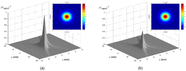
Figure 1: Representation of a Superluminal Modified Power Spectrum pulse, eq.(31).  Its total energy is finite (even without any truncation), and so it gets deformed while propagating, since its amplitude decreases with time.  In Fig.1a we represent, for $t=0$, the pulse corresponding to $\beta_{0}=33\,{\rm m}^{-1}$, $V=1.01c$, $a=10^{-12}\,$s and $q=10^{5}\,$m.  In Fig.1b it is depicted the same pulse after having travelled $50\;$km.

Other three important well known finite energy nondiffracting solutions can be obtained directly from the SMPS pulse:

— The first one, obtained from (31) by making $\beta_{0}=0$, is the so called[13] Superluminal Splash Pulse (SSP),

$$\Psi_{\rm SSP}(\rho,\zeta,\eta)\;=\;\frac{q\,X}{q+i\eta-Y}$$ (34)

— The other two are luminal pulses. By taking the limit $V\rightarrow c^{+}$ in the SMPS pulse (31), we get the well known[11] luminal Modified Power Spectrum (MPS) pulse

$$\Psi_{\rm MPS}(\rho,\zeta,\eta)\;=\;\frac{a\,q\,c\,e^{-i\beta_{0}\eta}}{(q+i\eta)(ac-i\zeta)+\rho^{2}}\,{\rm exp}\left(\frac{-\beta_{0}\rho^{2}}{ac-i\zeta}\right)$$ (35)

Finally, by taking the limit $V\rightarrow c^{+}$ and making $\beta_{0}=0$ in the SMPS pulse (or, equivalently, by making $\beta_{0}=0$ in the MPS pulse (35), or,instead, by taking the limit $V\rightarrow c^{+}$ in the SSP (34)), we obtain the well known[11] luminal Splash Pulse (SP) solution

$$\Psi_{\rm SP}(\rho,\zeta,\eta)\;=\;\frac{a\,q\,c}{(q+i\eta)(ac-i\zeta)+\rho^{2}}$$ (36)

It is also interesting to notice that the X and SFWM pulses can be obtained from the SSP and SMPS pulses (respectively) by making $q\rightarrow\infty$ in Eqs.(34) and (31). As a matter of fact, the solutions SSP and SMPS can be viewed as THE finite energy versions of the X and SFWM pulses, respectively.

Some characteristics of the SMPS pulse:

Let us examine the on-axis ($\rho=0$) behavior of the SMPS pulse.

On $\rho=0$ we have

$$\Psi_{\rm SMPS}(\rho=0,\zeta,\eta)\;=\;aqVe^{-i\beta_{0}z}[(aV-i\zeta)(q+i\eta)]^{-1}$$ (37)

From this expression, we can show that the longitudinal localization $\Delta z$, for $t=0$, of the SMPS pulse square magnitude is

$$\Delta z\;=\;2aV$$ (38)

If we now define the field depth $Z$ as the distance over which the pulse’s peak intensity is $50\%$ at least of its initial value, then we can obtain, from (37), the depth of field

$$Z_{\rm SMPS}\;=\;\frac{q}{2}$$ (39)

which depends only on $q$, as we expected since $q$ regulates the concentration of the spectrum around the line $\omega=Vk_{z}+2V\beta_{0}$.

Now, let us examine the maximum amplitude $M$ of the real part of (37), which for $z=Vt$ writes ($\zeta=0$ and $\eta=2z$):

$$M_{\rm SMPS}\equiv{\rm Re}[\Psi_{\rm SMPS}(\rho=0,z=Vt)]\;=\;\frac{\cos(2\beta_{0}z)-2(z/q)\sin(2\beta_{0}z)}{1+4(z/q)^{2}}$$ (40)

Initially, for $z=0$, $t=0$, one has $M=1$ and can also infer that:

(i) when $z/q<<1$, namely, when $z<<Z$, equation (40) becomes

$$M_{\rm SMPS}\approx\cos(2\beta_{0}z)\;\;\;\;\;{\rm for}\;\;z<<Z$$ (41)

and the pulse’s peak actually oscillates harmonically with “wavelength” $\Delta z_{0}=\pi/\beta_{0}$ and “period” $\Delta t_{0}=\pi/V\beta_{0}$, all along its field depth.

(ii) When $z/q>>1$, namely $z>>Z$, equation (40) becomes

$$M_{SMPS}\approx-\frac{\sin(2\beta_{0}z)}{2z/q}\;\;\;\;{\rm for}\;\;z>>Z$$ (42)

Therefore, beyond its depth of field, the pulse goes on oscillating with the same $\Delta z_{0}$, but its maximum amplitude decays proportionally to $z$.

In the next two Sections we are going to see an interesting application of the localized wave pulses.

3 Space-Time Focusing of X-shaped Pulses

In this Section we are going to show how one can in general use any known Superluminal solution, to obtain from it a large number of analytic expressions for space-time focused waves, endowed with a very strong intensity peak at the desired location.

The method presented here is a natural extension of that developed by A. Shaarawi et al.[20], where the space-time focusing was achieved by superimposing a discrete number of ordinary X-waves, characterized by different values $\theta$ of the axicon angle.

In this section, based on ref.[21], we will go on to more efficient superpositions for varying velocities $V$, related to $\theta$ through the known[3,4] relation $V=c/\cos\theta$. This enhanced focusing scheme has the advantage of yielding analytic (closed-form) expressions for the spatio-temporally focused pulses.

Let us start considering an axially symmetric ideal nondiffracting superluminal wave pulse $\psi(\rho,z-Vt)$ in a dispersionless medium, where $V=c/\cos\theta>c$ is the pulse velocity, $\theta$ being the axicon angle. As we have seen in the previous Section, pulses like these can be obtained by a suitable frequency superposition of Bessel beams.

Suppose that we have now $N$ waves of the type $\psi_{n}(\rho,z-Vn(t-tn))$, with different velocities $c<V_{1}<V_{2}<..<V_{N}$, and emitted at (different) times $t_{n}$; quantities $t_{n}$ being constants, while $n=1,2,...N$. The center of each pulse is located at $z=V_{n}(t-t_{n})$. To obtain a highly focused wave, we need all the wave components $\psi_{n}(\rho,z-Vn(t-tn))$ to reach the given point, $z=z_{\rm f}$, at the same time $t=t_{\rm f}$. On choosing $t_{1}=0$ for the slowest pulse $\psi_{1}$, it is easily seen that the peak of this pulse reaches the point $z=z_{\rm f}$ at the time $t_{\rm f}=z_{\rm f}/V_{1}$. So we obtain that, for each $\psi_{n}$, the instant of emission $t_{n}$ must be

$$t_{n}\;=\;\left(\frac{1}{V_{1}}-\frac{1}{V_{n}}\right)z_{\rm f}$$ (43)

With this, we can construct other exact solutions to the wave equation, given by

$$\Psi(\rho,z,t)\;=\;\int_{V_{\rm min}}^{V_{\rm max}}\,{\rm d}V\,A(V)\,\psi\left(\rho,z-V\left(t-\left(\frac{1}{V_{\rm min}}-\frac{1}{V}\right)z_{\rm f}\right)\right)\ ,$$ (44)

where $V$ is the velocity of the wave $\psi(\rho,z-Vt)$ in the integrand of (44). In the integration, $V$ is considered as a continuous variable in the interval $[V_{\rm min},V_{\rm max}]$. In eq. (2), $A(V)$ is the velocity-distribution function that specifies the contribution of each wave component (with velocity $V$) to the integration. The resulting wave $\Psi(\rho,z,t)$ can have a more or less strong amplitude peak at $z=z_{\rm f}$, at time $t_{\rm f}=z_{\rm f}/V_{\rm min}$, depending on $A(V)$ and on the difference $V_{\rm max}-V_{\rm min}$. Let us notice that also the resulting wavefield will propagate with a Superluminal peak velocity, depending on $A(V)$ too. In the cases when the velocity-distribution function is well concentrated around a certain velocity value, one can expect the wave (44) to increase its magnitude and spatial localization while propagating. Finally, the pulse peak acquires its maximum amplitude and localization at the chosen point $z=z_{\rm f}$, and at time $t=z_{\rm f}/V_{\rm min}$, as we know. Afterwards, the wave suffers a progressive spreading, and a decreasing of its amplitude.

3.1 Focusing Effects by Using Ordinary X-Waves

Here, we present a specific example by integrating (44) over the standard, ordinary[4] X-waves, $X=aV[(aV-i(z-Vt))^{2}+(V^{2}/c^{2}-1)\rho^{2}]^{-1/2}$. When using this ordinary X-wave, the largest spectral amplitudes are obtained for low frequencies. For this reason, one may expect that the solutions considered below will be suitable mainly for low frequency applications.

Let us choose, then, the function $\psi$ in the integrand of eq.(44) to be $\psi(\rho,z,t)\equiv X(\rho,z-V(t-(1/V_{\rm min}-1/V)z_{\rm f}))$, viz.

$$\psi(\rho,z,t)\equiv X\;=\;\displaystyle{\frac{aV}{\sqrt{\left[aV-i\left(z-V\left(t-\left(\frac{1}{V_{\rm min}}-\frac{1}{V}\right)z_{\rm f}\right)\right)\right]^{2}+\left(\frac{V^{2}}{c^{2}}-1\right)\rho^{2}}}}$$ (45)

After some manipulations, one obtains the analytic integral solution

$$\Psi(\rho,z,t)\;=\;\int_{V_{\rm min}}^{V_{\rm max}}\,\displaystyle{\frac{aV\,A(V)}{\sqrt{PV^{2}+QV+R}}}{\rm d}V$$ (46)

with

$$\begin{array}[]{l}P\;=\;\left[\left(a+i\left(t-\frac{z_{\rm f}}{V_{\rm min}}\right)\right)^{2}+\frac{\rho^{2}}{c^{2}}\right]\\ \\ Q\;=\;2\left(t-\frac{z_{\rm f}}{V_{\rm min}}-ai\right)(z-z_{\rm f})\\ \\ R\;=\;\left[-(z-z_{\rm f})^{2}-\rho^{2}\right]\end{array}$$ (47)

In what follows, we illustrate the behavior of some new spatio-temporally focused pulses, by taking into consideration some different velocity distributions $A(V)$. These new pulses are closed analytical exact solutions of the wave equation.

First example:

Let us consider our integral solution (46) with $A(V)=1\,{\rm s/m}$. In this case, the contribution of the X-waves is the same for all velocities in the allowed range $[V_{\rm min},V_{\rm max}]$.

Using identity 2.264.2 listed in ref.[19], we get the particular solution

$$\begin{array}[]{clcr}\Psi(\rho,z,t)\!\!&=\displaystyle{\frac{a}{P}}\,\displaystyle{\left(\sqrt{PV_{\rm max}^{2}+QV_{\rm max}+R}-\sqrt{PV_{\rm min}^{2}+QV_{\rm min}+R}\,\right)}\\ \\ &\;\;\;\displaystyle{+\frac{a\,Q}{2P^{3/2}}\,{\rm ln}\left(\frac{2\,\sqrt{P(PV_{\rm min}^{2}+QV_{\rm min}+R)}+2PV_{\rm min}+Q}{2\,\sqrt{P(PV_{\rm max}^{2}+QV_{\rm max}+R)}+2PV_{\rm max}+Q}\right)}\ ,\end{array}$$ (48)

where $P$, $Q$ and $R$ are given in eq.(47). A 3-dimensional (3D) plot of this function is provided in Fig.2; where we have chosen $a=10^{-12}$ s,  $V_{\rm min}=1.001\;c$,  $V_{\rm max}=1.005\;c$ and $z_{\rm f}=200\;$cm. It can be seen that this solution exhibits a rather evident space-time focusing. An initially spread-out pulse (shown for $t=0$) becomes highly localized at $t=t_{\rm f}=z_{\rm f}/V_{\rm min}=6.66\;$ns, the pulse peak amplitude at $z_{\rm f}$ being $40.82$ times greater than the initial one. In addition, at the focusing time $t_{\rm f}$ the field is much more localized than at any other times. The velocity of this pulse is approximately $V=1.003\;c$.

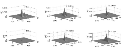
Figure 2: Space-time evolution of the Superluminal pulse represented by eq.(48); the chosen parameter values are $a=10^{-12}\;$s;  $V_{\rm min}=1.001\;c$;  $V_{\rm max}=1.005\;c$ while the focusing point is at $z_{\rm f}=200\;$cm.  One can see that this solution is associated with a rather good spatio-temporal focusing.  The field amplitude at $z=z_{\rm f}$ is 40.82 times larger than the initial one.  The field amplitude is normalized at the space-time point $\rho=0,\ z=z_{\rm f},\ t=t_{\rm f}$.

Second example:

In this case we choose $A(V)=1/V\,\,({\rm s/m})$, and, using the identity 2.261 in ref.[19], eq.(46) gives

$$\Psi(\rho,z,t)\;=\;\displaystyle{\frac{a}{\sqrt{P}}\,{\rm ln}\left(\frac{2\,\sqrt{P(PV_{\rm max}^{2}+QV_{\rm max}+R)}+2PV_{\rm max}+Q}{2\,\sqrt{P(PV_{\rm min}^{2}+QV_{\rm min}+R)}+2PV_{\rm min}+Q}\right)}\ .$$ (49)

Other exact closed-form solutions can be obtained[21] considering, for instance, velocity distributions like $A(V)=1/V^{2}$ and $A(V)=1/V^{3}$.

Actually, we can construct many others spatio-temporally focused pulses from the above solutions, just by taking their time derivatives (of any order). It is also possible to show[21] that the new solutions obtained in this way have their spectra shifted towards higher frequencies.

4 Chirped Optical X-Type Pulses in Material Media

The theory of the localized waves was initially developed for free space (vacuum). In 1996, Sõnajalg et al.[5] showed that the localized wave theory can be extended to include (unbounded) dispersive media. This was obtained by making the axicon angle of the Bessel beams (BBs) vary with the frequency[5-7] in such a way that a suitable frequency superposition of these beams does compensate for the material dispersion. Soon after this idea was reported, many interesting nondiffracting/nondispersive pulses were obtained theoretically[5-7] and experimentally[5].

In spite of this extended method to be of remarkable importance, working well in theory, its experimental implementation is not so simple.

In 2004 Zamboni-Rached et al.[22] developed a simpler way to obtain pulses capable of recovering their spatial shape, both transversally and longitudinally, after some propagation. It consisted in using chirped optical X-typed pulses, while keeping the axicon angle fixed. Let us recall that, by contrast, chirped Gaussian pulses in unbounded material media may recover only their longitudinal shape, since they undergo a progressive transverse spreading while propagating.

The present section is devoted to this approach.

Let us start with an axis-symmetric Bessel beam in a material medium with refractive index $n(\omega)$:

$$\psi(\rho,z,t)\;=\;J_{0}(k_{\rho}\rho)\,\exp(i\beta z)\,\exp(-i\omega t)\;,$$ (50)

where it must be obeyed the condition  $k_{\rho}^{2}=n^{2}(\omega)\omega^{2}/c^{2}-\beta^{2}$,  which connects among themselves the transverse and longitudinal wave numbers $k_{\rho}$ and $\beta$, and the angular frequency $\omega$. In addition, we impose that $k_{\rho}^{2}\geq 0$ and $\omega/\beta\geq 0$, to avoid a nonphysical behavior of the Bessel function $J_{0}(.)$ and to confine ourselves to forward propagation only.

Once the conditions above are satisfied, we have the liberty of writing the longitudinal wave number as $\beta=(n(\omega)\omega\cos\theta)/c$ and, therefore, $k_{\rho}=(n(\omega)\omega\sin\theta)/c$; where (as in the free space case) $\theta$ is the axicon angle of the Bessel beam.

Now we can obtain a X-shaped pulse by performing a frequency superposition of these Bessel beams [BB], with $\beta$ and $k_{\rho}$ given by the previous relations:

$$\Psi(\rho,z,t)\;=\;\int_{-\infty}^{\infty}\,S(\omega)\,J_{0}\left(\frac{n(\omega)\omega}{c}\sin\theta\,\rho\right)\,\exp[i\beta(\omega)z]\,\exp(-i\omega t)\,{\rm d}\omega\;,$$ (51)

where $S(\omega)$ is the frequency spectrum, and the axicon angle is kept constant.

One can see that the phase velocity of each BB in our superposition (51) is different, and given by $V_{\rm phase}=c/(n(\omega)\cos\theta)$. So, the pulse represented by eq.(51) will suffer dispersion during its propagation.

As we said, the method developed by Sõnajalg et al.[5] and explored by others[6,7], to overcome this problem, consisted in regarding the axicon angle $\theta$ as a function of the frequency, in order to obtain a linear relationship between $\beta$ and $\omega$.

Here, however, we wish to work with a fixed axicon angle, and we have to find out another way for avoiding dispersion and diffraction along a certain propagation distance. To do that, we might choose a chirped gaussian spectrum $S(\omega)$ in eq.(51)

$$S(\omega)\;=\;\frac{T_{0}}{\sqrt{2\pi(1+iC)}}\,\,\exp[-q^{2}(\omega-\omega_{0})^{2}]\;\;\;\;{\rm with}\;\;\;\;\;q^{2}\;=\;\frac{T_{0}^{2}}{2(1+iC)}\;,$$ (52)

where $\omega_{0}$ is the central frequency of the spectrum, $T_{0}$ is a constant related with the initial temporal width, and $C$ is the chirp parameter (we chose as temporal width the half-width of the relevant gaussian curve when its heigth equals $1/e$ times its full heigth). Unfortunately, there is no analytical solution to eq.(51) with $S(\omega)$ given by eq.(52), so that some approximations are to be made.

Then, let us assume that the spectrum $S(\omega)$, in the surrounding of the carrier frequency $\omega_{0}$ , is enough narrow that $\Delta\omega/\omega_{0}<<1$, so to ensure that $\beta(\omega)$ can be approximated by the first three terms of its Taylor expansion in the vicinity of $\omega_{0}$: That is,  $\beta(\omega)\approx\beta(\omega_{0})+\beta^{\prime}(\omega)|_{\omega_{0}}\,(\omega-\omega_{0})+(1/2)\beta^{\prime\prime}(\omega)|_{\omega_{0}}\,(\omega-\omega_{0})^{2}$;  where, after using $\beta=n(\omega)\omega\cos\theta/c$, it results that

$$\frac{\partial\beta}{\partial\omega}\;=\;\frac{\cos\theta}{c}\left[n(\omega)+\omega\,\frac{\partial n}{\partial\omega}\right]\,;\ \ \ \frac{\partial^{2}\beta}{\partial\omega^{2}}\;=\;\frac{\cos\theta}{c}\left[2\frac{\partial n}{\partial\omega}+\omega\frac{\partial^{2}n}{\partial\omega^{2}}\right]\;.$$ (53)

As we know, $\beta^{\prime}(\omega)$ is related to the pulse group-velocity by the relation $Vg=1/\beta^{\prime}(\omega)$. Here we can see the difference between the group-velocity of the X-type pulse (with a fixed axicon angle) and that of a standard gaussian pulse. Such a difference is due to the factor $\cos\theta$ in eq.(53). Because of it, the group-velocity of our X-type pulse is always greater than the gaussian’s. In other words, $(V_{\rm g})_{\rm X}=(1/\cos\theta)(V_{\rm g})_{gauss}$.

We also know that the second derivative of $\beta(\omega)$ is related to the group-velocity dispersion (GVD) $\beta_{2}$ by $\beta_{2}=\beta^{\prime\prime}(\omega)$.

The GVD is responsible for the temporal (longitudinal) spreading of the pulse. Here one can see that the GVD of the X-type pulse is always smaller than that of the standard gaussian pulses, due the factor $\cos\theta$ in eq.(53). Namely: $(\beta_{2})_{\rm X}=\cos\theta(\beta_{2})_{\rm gauss}$.

Using the above results, we can write

$$\begin{array}[]{clcr}\Psi(\rho,z,t)\!\!&=\displaystyle{\frac{T_{0}\,\,\exp[i\beta(\omega_{0})z]\,\exp(-i\omega_{0}t)}{\sqrt{2\pi(1+iC)}}\,\int_{-\infty}^{\infty}{\rm d}\omega\,J_{0}\left(\frac{n(\omega)\omega}{c}\sin\theta\,\rho\right)}\\ \\ &\;\;\;\times\,\displaystyle{\exp\left\{i\frac{(\omega-\omega_{0})}{V_{\rm g}}\left[z-V_{\rm g}t\right]\right\}\,\exp\left\{(\omega-\omega_{0})^{2}\left[\frac{i\beta_{2}}{2}z-q^{2}\right]\right\}}\;.\end{array}$$ (54)

The integral in eq.(54) cannot be solved analytically, but it is enough for us to obtain the pulse behavior. Let us analyze the pulse for $\rho=0$. In this case we obtain:

$$\Psi(\rho=0,z,t)\;=\;\displaystyle{\frac{T_{0}\,\exp[i\beta(\omega_{0})z]\,\exp(-i\omega_{0}t)}{\sqrt{T_{0}^{2}-i\beta_{2}(1+iC)z}}\,\exp\left[\frac{-(z-V_{\rm g}t)^{2}(1+iC)}{2V_{\rm g}^{2}[T_{0}^{2}-i\beta_{2}(1+iC)z]}\right]}\;.$$ (55)

From eq.(55) one can immediately see that the initial temporal width of the pulse intensity is $T_{0}$ and that, after a propagation distance $z$, the time-width $T_{1}$ becomes

$$\frac{T_{1}}{T_{0}}\;=\;\left[\left(1+\frac{C\beta_{2}z}{T_{0}^{2}}\right)^{2}+\left(\frac{\beta_{2}z}{T_{0}^{2}}\right)^{2}\right]^{1/2}\;.$$ (56)

Relation (56) describes the pulse spreading-behavior. One can easily show that such a behavior depends on the sign (positive or negative) of the product $\beta_{2}C$, as is well known for the standard gaussian pulses[23].

In the case $\beta_{2}C>0$, the pulse will monotonically become broader and broader with the distance $z$. On the other hand, if $\beta_{2}C<0$ the pulse will suffer, in a first stage, a narrowing, and then it will spread during the rest of its propagation. So, there will be a certain propagation distance AT which the pulse will recover its initial temporal width ($T_{1}=T_{0}$). From relation (56), we can find this distance $Z_{T1=T_{0}}$ (considering $\beta_{2}C<0$) to be

$$Z_{T_{1}=T_{0}}\;=\;\frac{-2CT_{0}^{2}}{\beta_{2}(C^{2}+1)}\;.$$ (57)

One may notice that the maximum distance at which our chirped pulse, with given $T_{0}$ and $\beta_{2}$, may recover its initial temporal width can be easily evaluated from eq.(57), and it results to be $L_{\rm disp}=T_{0}^{2}/\beta_{2}$. We shall call such a maximum value $L_{\rm disp}$ the “dispersion length”. It is the maximum distance the X-type pulse may travel while recovering its initial longitudinal shape. Obviously, if we want the pulse to reassume its longitudinal shape at some desired distance $z<L_{\rm disp}$, we have just to suitably choose the value of the chirp parameter.

Let us emphasize that the property of recovering its own initial temporal (or longitudinal) width may be verified to exist also in the case of chirped standard gaussian pulses. However, the latter will suffer a progressive transverse spreading, which will not be reversible. The distance at which a gaussian pulse doubles its initial transverse width $w_{0}$ is $z_{\rm diff}=\sqrt{3}\pi w_{0}^{2}/\lambda_{0}$, where $\lambda_{0}$ is the carrier wavelength. Thus, we can see that optical gaussian pulses with great transverse localization will get spoiled in a few centimeters or even less.

Now we shall show that it is possible to recover also the transverse shape of the chirped X-type pulse intensity; actually, it is possible to recover its entire spatial shape after a distance $Z_{T_{1}=T_{0}}$.

To see this, let us go back to our integral solution (54), and perform the change of coordinates  $(z,t)\rightarrow(\Delta z,t_{c}=z_{c}/V_{\rm g})$, with

$$\left\{\begin{array}[]{l}z\;=\;z_{c}+\Delta z\\ \\ \displaystyle{t=t_{c}\equiv\frac{z_{c}}{V_{\rm g}}}\end{array}\right.$$ (58)

where $z_{c}$ is the center of the pulse ($\Delta z$ is the distance from such a point), and $t_{c}$ is the time at which the pulse center is located at $z_{c}$. What we are going to do is comparing our integral solution (54), when $z_{c}=0$ (initial pulse), with that when $z_{c}=Z_{T_{1}=T_{0}}=-2CT_{0}^{2}/(\beta_{2}(C_{2}+1))$.

In this way, the solution (54) can be written, when $z_{c}=0$, as

$$\begin{array}[]{clcr}\Psi(\rho,z_{c}=0,\Delta z)\!\!&=\displaystyle{\frac{T_{0}\,\,\,\exp(i\beta_{0}\Delta z)}{\sqrt{2\pi(1+iC)}}}\,\int_{-\infty}^{\infty}{\rm d}\omega\,J_{0}(k_{\rho}(\omega)\rho)\,\exp\left[\frac{-T_{0}^{2}\,(\omega-\omega_{0})^{2}}{2(1+C^{2})}\right]\\ \\ \\ &\;\;\;\displaystyle{\times\,\exp\left\{i\left[\frac{(\omega-\omega_{0})\Delta z}{V_{\rm g}}+\frac{(\omega-\omega_{0})^{2}\beta_{2}\Delta z}{2}+\frac{(\omega-\omega_{0})^{2}T_{0}^{2}C}{2(1+C^{2})}\right]\right\}}\\ \end{array}$$ (59)

where we have taken the value $q$ given by (52).

To verify that the pulse intensity recovers its entire original form at $z_{c}=Z_{T_{1}=T_{0}}=-2\,CT_{0}^{2}/[\beta_{2}(C^{2}+1)]$, we can analyze our integral solution at that point, obtaining

$$\begin{array}[]{l}\Psi(\rho,z_{c}=Z_{T_{1}=T_{0}},\Delta z)\ =\ \displaystyle{\frac{T_{0}\,\,\displaystyle{\exp\left\{i\beta_{0}\left[z_{c}-\Delta z^{\prime}-\frac{cz_{c}}{\cos\theta\,n(\omega_{0})V_{\rm g}}\right]\right\}}}{\sqrt{2\pi(1+iC)}}}\\ \\ \\ \times\displaystyle{\int_{-\infty}^{\infty}}\displaystyle{{\rm d}\omega\,J_{0}(k_{\rho}(\omega)\rho)\,\exp\left[\frac{-T_{0}^{2}\,(\omega-\omega_{0})^{2}}{2(1+C^{2})}\right]}\\ \\ \\ \displaystyle{\times\,\exp\left\{-i\left[\frac{(\omega-\omega_{0})\Delta z^{\prime}}{V_{\rm g}}+\frac{(\omega-\omega_{0})^{2}\beta_{2}\Delta z^{\prime}}{2}+\frac{(\omega-\omega_{0})^{2}T_{0}^{2}C}{2(1+C^{2})}\right]\right\}}\\ \end{array}$$ (60)

where we put $\Delta z=-\Delta z^{\prime}$.  In this way, one immediately sees that

$$|\Psi(\rho,z_{c}=0,\Delta z)|^{2}=|\Psi(\rho,z_{c}=Z_{T_{1}=T_{0}},-\Delta z)|^{2}\;.$$ (61)

Therefore, from eq.(61) it is clear that the chirped optical X-type pulse intensity will recover its original three-dimensional form, with just a longitudinal inversion at the pulse center: The present method being, in this way, a simple and effective procedure for compensating the effects of diffraction and dispersion in an unbounded material medium; and a method simpler than the one of varying the axicon angle with the frequency.

Let us stress that we can choose the distance $z=Z_{T_{1}=T_{0}}\leq L_{\rm disp}$ at which the pulse will take on again its spatial shape by choosing a suitable value of the chirp parameter.

Till now, we have shown that the chirped X-type pulse recovers its three-dimensional shape after some distance, and we have also obtained an analytic description of the pulse longitudinal behavior (for $\rho=0$) during propagation, by means of eq.(55). However, one does not get the same information about the pulse transverse behavior: We just know that it is recovered at $z=Z_{T_{1}=T_{0}}$.

So, to complete the picture, it would be interesting if we could get also the transverse behavior in the plane of the pulse center $z=V_{\rm g}t$. In that way, we would obtain quantitative information about the evolution of the pulse-shape during its entire propagation.

We will not examine the mathematical details here; we just affirm that THE transverse behavior of the pulse (in the plane $z=z_{c}=V_{\rm g}t$) during its whole propagation can approximately be described by

$$\begin{array}[]{l}\Psi(\rho,z=z_{c},t=z_{c}/V_{\rm g})\,\approx\,\displaystyle{\frac{T_{0}\,\,\,\exp[i\beta(\omega_{0})z]\,\exp(-i\omega_{0}t)}{\sqrt{2\pi(1+iC)}}\,\,\frac{\exp\displaystyle{\left[\frac{-\tan^{2}\theta\,\rho^{2}}{8\,V_{\rm g}^{2}(-i\beta_{2}z_{c}/2\,+q^{2})}\right]}}{\sqrt{-i\beta_{2}z_{c}/2\,+q^{2}}}}\\ \\ \\ \times\,\displaystyle{\left[\Gamma(1/2)J_{0}\left(\frac{n(\omega_{0})\,\omega_{0}\,\sin\theta\,\rho}{c}\right)I_{0}\left(\frac{\tan^{2}\theta\,\rho^{2}}{8\,V_{\rm g}^{2}(-i\beta_{2}z_{c}/2\,+q^{2})}\right)\right.}\\ \\ \\ \left.+\displaystyle{2\sum_{p=1}^{\infty}\frac{2^{p}\Gamma(p+1/2)\Gamma(p+1)}{\Gamma(2p+1)}\,\,J_{2p}\left(\frac{n(\omega_{0})\,\omega_{0}\,\sin\theta\,\rho}{c}\right)I_{2p}\left(\frac{\tan^{2}\theta\,\rho^{2}}{8\,V_{\rm g}^{2}(-i\beta_{2}z_{c}/2\,+q^{2})}\right)}\right]\\ \end{array}$$ (62)

where $I_{p}(.)$ is the modified Bessel function of the first kind of order $p$, quantity $\Gamma(.)$ being the gamma function and $q$ given by (52).

The interested reader can consult ref.[22] for details on how to obtain eq.(LABEL:S4trans1) from eq.(54).

At a first sight, this solution could appear very complicated, but the series in its r.h.s. gives a negligible contribution. This fact renders our solution (LABEL:S4trans1) of important practical interest and we will use it in the following.

For additional information about the transverse pulse evolution (extracted from eq.(LABEL:S4trans1)), the reader can consult again ref.[22] . In the same reference, it is analyzed the effect of a finite aperture generation on the chirped X-type pulses.

4.1 An example: Chirped Optical X-typed pulse in bulk fused Silica

For a bulk fused Silica, the refractive index $n(\omega)$ can be approximated by the Sellmeier equation[23]

$$n^{2}(\omega)\;=\;\displaystyle{1\,+\,\sum_{j=1}^{N}\,\frac{B_{j}\,\omega_{j}^{2}}{\omega_{j}^{2}-\omega^{2}}}\;,$$ (63)

where $\omega_{j}$ are the resonance frequencies, $B_{j}$ the strength of the $j$th resonance, and $N$ the total number of the material resonances that appear in the frequency range of interest. For our purposes it is appropriate to choose $N=3$, which yields, for bulk fused silica[23], the values  $B_{1}=0.6961663$;  $B_{2}=0.4079426$;  $B_{3}=0.8974794$;  $\lambda_{1}=0.0684043\;\mu\;$m;  $\lambda_{2}=0.1162414\;\mu\;$m;  and $\lambda_{3}=9.896161\;\mu\;$m.

Now, let us consider in this medium a chirped X-type pulse, with $\lambda_{0}=0.2\,\mu$m,  $T_{0}=0.4\;$ps,  $C=-1$ and with an axicon angle $\theta=0.00084\;$rad, which correspond to an initial central spot with $\Delta\rho_{0}=0.117\;$mm.

We get from eqs. (55) and (LABEL:S4trans1), the longitudinal and transverse pulse evolution, which are represented by Fig.3

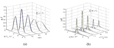
Figure 3: (a): Longitudinal-shape evolution of a chirped X-type pulse, propagating in fused silica with $\lambda_{0}=0.2\mu\;$m,  $T_{0}=0.4\;$ps,  $C=-1$ and axicon angle $\theta=0.00084\;$rad, which correspond to an initial transverse width of $\Delta\rho_{0}=0.117\;$mm.   (b): Transverse-shape evolution for the same pulse.

From Fig.3(a), we can notice that, initially, the pulse suffers a longitudinal narrowing with an increase of intensity till the position $z=T_{0}^{2}/2\beta_{2}=0.186$m. After this point, the pulse starts to broaden decreasing its intensity and recovering its entire longitudinal shape (width and intensity) at the point $z=T_{0}^{2}/\beta_{2}=0.373$m, as it was predicted.

At the same time, from Fig.3(b), one can notice that the pulse maintains its transverse width $\Delta\rho=2.4\,c/(n(\omega_{0})\omega_{0}\sin\theta)=0.117\;$mm  (because $T_{0}\omega_{0}>>1$) during its entire propagation; however, the same does not occur with the pulse intensity. Initially the pulse suffers an increase of intensity till the position $z_{c}=T_{0}^{2}/2\beta_{2}=0.186$m; after this point, the intensity starts to decrease, and the pulse recovers its entire transverse shape at the point $z_{c}=T_{0}^{2}/\beta_{2}=0.373$m, as it was expected by us. Here we have skipped the series on the r.h.s. of eq.(LABEL:S4trans1), because, as we already said, it yields a negligible contribution.

Summarizing, from Fig.3, we can see that the chirped X-type pulse recovers totally its longitudinal and transverse shape at the position $z=L_{\rm Disp}=T^{2}_{0}/\beta_{2}=0.373\;$m, as we expected.

Let us recall that a chirped gaussian pulse may just recover its longitudinal width, but with an intensity decrease, at the position given by $z=Z_{T_{1}=T_{0}}=L_{\rm disp}=T^{2}_{0}/\beta_{2}$. Its transverse width, on the other hand, suffers a progressive and irreversible spreading.

5 Modeling the Shape of Stationary Wave Fields: Frozen Waves

In this Section we develop a very simple method[10,16,17], by having recourse to superpositions of forward propagating and equal-frequency Bessel beams, that allows one controlling the longitudinal beam-intensity shape within a chosen interval $0\leq z\leq L$, where $z$ is the propagation axis and $L$ can be much greater than the wavelength $\lambda$ of the monochromatic light (or sound) which is being used. Inside such a space interval, indeed, we succeed in constructing a stationary envelope whose longitudinal intensity pattern can approximately assume any desired shape, including, for instance, one or more high-intensity peaks (with distances between them much larger than $\lambda$); and which results —in addition— to be naturally endowed also with a good transverse localization. Since the intensity envelopes remains static, i.e. with velocity $V=0$, we call “Frozen Waves” (FW) such new solutions[10,16,17] to the wave equations.

Although we are dealing here with exact solutions of the scalar wave equation, vectorial solutions of the same kind for the electromagnetic field can be obtained, since solutions to Maxwell’s equations follow naturally from the scalar wave equation solutions[24,25].

First, we present the method considering lossless media[16,17] and, in the second part of this section, we extend the method to absorbing media[10].

5.1 Stationary wavefields with arbitrary longitudinal shape in lossless media, obtained by superposing equal-frequency Bessel beams

Let us start from the well-known axis-symmetric zeroth order Bessel beam solution to the wave equation:

$$\psi(\rho,z,t)\;=\;J_{0}(k_{\rho}\rho)e^{i\beta z}e^{-i\omega t}$$ (64)

with

$$k_{\rho}^{2}=\frac{\omega^{2}}{c^{2}}-\beta^{2}\;,$$ (65)

where $\omega$, $k_{\rho}$ and $\beta$ are the angular frequency, the transverse and the longitudinal wave numbers, respectively. We also impose the conditions

$$\omega/\beta>0\;\;\;{\rm and}\;\;\;k_{\rho}^{2}\geq 0$$ (66)

(which imply $\omega/\beta\geq c$) to ensure forward propagation only (with no evanescent waves), as well as a physical behavior of the Bessel function $J_{0}$.

Now, let us make a superposition of $2N+1$ Bessel beams with the same frequency $\omega_{0}$, but with different (and still unknown) longitudinal wave numbers $\beta_{m}$:

$${\Psi(\rho,z,t)\;=\;e^{-i\,\omega_{0}\,t}\,\sum_{m=-N}^{N}A_{m}\,J_{0}(k_{\rho\,m}\rho)\,e^{i\,\beta_{m}\,z}}\;,$$ (67)

where thye $m$ represent integer numbers and the $A_{m}$ are constant coefficients. For each $m$, the parameters $\omega_{0}$, $k_{\rho\,m}$ and $\beta_{m}$ must satisfy (65), and, because of conditions (66), when considering $\omega_{0}>0$, we must have

$$0\leq\beta_{m}\leq\frac{\omega_{0}}{c}\;.$$ (68)

Let us now suppose that we wish $|\Psi(\rho,z,t)|^{2}$, given by eq.(67), to assume on the axis $\rho=0$ the pattern represented by a function $|F(z)|^{2}$, inside the chosen interval $0\leq z\leq L$. In this case, the function $F(z)$ can be expanded, as usual, in a Fourier series:

$$F(z)\;=\;\sum_{m=-\infty}^{\infty}\,B_{m}\,e^{i\,\frac{2\pi}{L}\,m\,z}\;,$$

where

$$B_{m}\;=\;\frac{1}{L}\displaystyle{\int_{0}^{L}\,F(z)\,e^{-i\,\frac{2\pi}{L}\,m\,z}\,{\rm d}\,z}\ .$$

More precisely, our goal is finding out, now, the values of the longitudinal wave numbers $\beta_{m}$ and the coefficients $A_{m}$ of (67), in order to reproduce approximately, within the said interval $0\leq z\leq L$ (for $\rho=0$), the predetermined longitudinal intensity-pattern $|F(z)|^{2}$.  Namely, we wish to have

$$\left|\,\sum_{m=-N}^{N}A_{m}e^{i\,\beta_{m}\,z}\right|^{\,2}\approx|F(z)|^{\,2}\;\;\;\;{\rm with}\;\;\;0\leq z\leq L\;.$$ (69)

Looking at eq.(69), one might be tempted to take $\beta_{m}=2\pi m/L$, thus obtaining a truncated Fourier series, expected to represent approximately the desired pattern $F(z)$.  Superpositions of Bessel beams with $\beta_{m}=2\pi m/L$ have been actually used in some works to obtain a large set of transverse amplitude profiles[26]. However, for our purposes, this choice is not appropriate, due to two principal reasons:  1) It yields negative values for $\beta_{m}$ (when $m<0$), which implies backwards propagating components (since $\omega_{0}>0$);  2) In the cases when $L>>\lambda_{0}$, which are of our interest here, the main terms of the series would correspond to very small values of $\beta_{m}$, which results in a very short field-depth of the corresponding Bessel beams (when generated by finite apertures), preventing the creation of the desired envelopes far form the source.

Therefore, we need to make a better choice for the values of $\beta_{m}$, which permits forward propagation components only, and a good depth of field.  This problem can be solved by putting

$$\beta_{m}\;=\;Q+\frac{2\,\pi}{L}\,m\;,$$ (70)

where $Q>0$ is a value to be chosen (as we shall see) according to the given experimental situation, and the desired degree of transverse field localization.  Due to eq.(68), we get

$$0\leq Q\pm\frac{2\,\pi}{L}\,N\leq\frac{\omega_{0}}{c}\;.$$ (71)

Inequality (71), can be used to determine the maximum value of $m$, that we call $N_{\rm max}$, once $Q$, $L$ and $\omega_{0}$ have been chosen.

As a consequence, for getting a longitudinal intensity pattern approximately equal to the desired one, $|F(z)|^{2}$, in the interval $0\leq z\leq L$, eq.(67) should be rewritten as

$${\Psi(\rho=0,z,t)\;=\;e^{-i\,\omega_{0}\,t}\,e^{i\,Q\,z}\,\sum_{m=-N}^{N}A_{m}\,e^{i\,\frac{2\pi}{L}m\,z}}\;,$$ (72)

with

$$A_{m}\;=\;\frac{1}{L}\displaystyle{\int_{0}^{L}\,F(z)\,e^{-i\,\frac{2\pi}{L}\,m\,z}\,{\rm d}\,z}\;.$$ (73)

Obviously, one obtains only an approximation to the desired longitudinal pattern, because the trigonometric series (72) is necessarily truncated ($N\leq N_{\rm max}$). Its total number of terms, let us repeat, will be fixed once the values of $Q$, $L$ and $\omega_{0}$ are chosen.

When $\rho\neq 0$, the wavefield $\Psi(\rho,z,t)$ becomes

$${\Psi(\rho,z,t)\;=\;e^{-i\,\omega_{0}\,t}\,e^{i\,Q\,z}\,\sum_{m=-N}^{N}A_{m}\,J_{0}(k_{\rho\,m}\,\rho)\,e^{i\,\frac{2\pi}{L}m\,z}}\;,$$ (74)

with

$$k_{\rho\,m}^{2}\;=\;\omega_{0}^{2}-\left(Q+\frac{2\pi\,m}{L}\right)^{2}\;.$$ (75)

The coefficients $A_{m}$ will yield the amplitudes and the relative phases of each Bessel beam in the superposition.

Because we are adding together zero-order Bessel functions, we can expect a high field concentration around $\rho=0$. Moreover, due to the known non-diffractive behavior of the Bessel beams, we expect that the resulting wavefield will preserve its transverse pattern in the entire interval $0\leq z\leq L$.

The methodology developed here deals with the longitudinal intensity pattern control. Obviously, we cannot get a total 3D control, due the fact that the field must obey the wave equation. However, we can use two ways to have some control over the transverse behavior too. The first is through the parameter $Q$ of eq.(70).  Actually, we have some freedom in the choice of this parameter, and FWs representing the same longitudinal intensity pattern can possess different values of $Q$. The important point is that, in superposition (74), using a smaller value of $Q$ makes the Bessel beams possess a higher transverse concentration (because, on decreasing the value of $Q$, one increases the value of the Bessel beams transverse wave numbers), and this will reflect in the resulting field, which will present a narrower central transverse spot. The second way to control the transverse intensity pattern is using higher order Bessel beams, and we shall show this in Section 5.1.1.

Now, let us present a few examples of our methodology.

First example:

Let us suppose that we wish an optical wavefield with $\lambda_{0}=0.632\;\mu$m, i.e. with $\omega_{0}=2.98\times 10^{15}\;$Hz, whose longitudinal pattern (along its $z$-axis) in the range $0\leq z\leq L$ is given by the function

$$F(z)\;=\;\left\{\begin{array}[]{clr}-4\,\,\displaystyle{\frac{(z-l_{1})(z-l_{2})}{(l_{2}-l_{1})^{2}}}&{\rm for}\;\;\;l_{1}\leq z\leq l_{2}\\ \\ \;\;\;\;\;\;\;\;1&{\rm for}\;\;\;l_{3}\leq z\leq l_{4}\\ \\ -4\,\,\displaystyle{\frac{(z-l_{5})(z-l_{6})}{(l_{6}-l_{5})^{2}}}&{\rm for}\;\;\;l_{5}\leq z\leq l_{6}\\ \\ \;\;\;\;\;\;\;\;0&\mbox{elsewhere}\ ,\end{array}\right.$$ (76)

where $l_{1}=L/5-\Delta z_{12}$ and $l_{2}=L/5+\Delta z_{12}$ with $\Delta z_{12}=L/50$; while $l_{3}=L/2-\Delta z_{34}$ and $l_{4}=L/2+\Delta z_{34}$ with $\Delta z_{34}=L/10$; and, at last, $l_{5}=4L/5-\Delta z_{56}$ and $l_{6}=4L/5+\Delta z_{56}$ with $\Delta z_{56}=L/50$. In other words, the desired longitudinal shape, in the range $0\leq z\leq L$, is a parabolic function for $l_{1}\leq z\leq l_{2}$, a unitary step function for $l_{3}\leq z\leq l_{4}$, and again a parabola in the interval $l_{5}\leq z\leq l_{6}$, being zero elsewhere (within the interval $0\leq z\leq L$, as we said). In this example, let us put $L=0.2\;$m.

We can then easily calculate the coefficients $A_{m}$, which appear in the superposition (74), by inserting eq.(76) into eq.(73). Let us choose, for instance, $Q=0.999\,\omega_{0}/c$. This choice permits the maximum value $N_{\rm max}=316$ for $m$, as one can infer from eq.(71). Let us emphasize that one is not compelled to use just $N=316$, but can adopt for $N$ any values smaller than it; more generally, any value smaller than that calculated via inequality (71). Of course, WHEN using the maximum value allowed for $N$, one gets a better result.

In the present case, let us adopt the value $N=30$. In Fig.4(a) we compare the intensity of the desired longitudinal function $F(z)$ with that of the Frozen Wave,  $\Psi(\rho=0,z,t)$,  obtained from eq.(72) by adopting the mentioned value $N=30$.

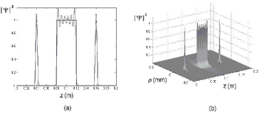
Figure 4: (a) Comparison between the intensity of the desired longitudinal function $F(z)$ and that of our Frozen Wave (FW),  $\Psi(\rho=0,z,t)$,  obtained from eq.(72). The solid line represents the function $F(z)$, and the dotted one our FW. (b) 3D-plot of the field-intensity of the FW chosen in this case by us.

One can verify that a good agreement between the desired longitudinal behavior and our approximate FW is already got with $N=30$. The use of higher values for $N$ can only improve the approximation.  Figure 4(b) shows the 3D-intensity of our FW, given by eq.(74). One can observe that this field possesses the desired longitudinal pattern, while being endowed with a good transverse localization.

Second example (controlling the transverse shape too):

We wish to take advantage of this example for addressing an important question:  We can expect that, for a desired longitudinal pattern of the field intensity, by choosing smaller values of the parameter $Q$ one will get FWs with narrower transverse width [for the same number of terms in the series entering eq.(74)], because of the fact that the Bessel beams in eq.(74) will possess larger transverse wave numbers, and, consequently, higher transverse concentrations.  We can verify this expectation by considering, for instance, inside the usual range $0\leq z\leq L$, the longitudinal pattern represented by the function

$$F(z)\;=\;\left\{\begin{array}[]{clr}-4\,\,\displaystyle{\frac{(z-l_{1})(z-l_{2})}{(l_{2}-l_{1})^{2}}}&{\rm for}\;\;\;l_{1}\leq z\leq l_{2}\\ \\ \;\;\;\;\;\;\;\;0&\mbox{elsewhere}\end{array}\right.\;,$$ (77)

with $l_{1}=L/2-\Delta z$ and $l_{2}=L/2+\Delta z$. Such a function has a parabolic shape, with its peak centered at $L/2$ and with longitudinal width $2\Delta z/\sqrt{2}$. By adopting $\lambda_{0}=0.632\;\mu$m (that is, $\omega_{0}=2.98\times 10^{15}\;$Hz), let us use the superposition (74) with two different values of $Q$:  We shall obtain two different FWs that, in spite of having the same longitudinal intensity pattern, will possess different transverse localizations. Namely, let us consider $L=0.06\,$m and $\Delta z=L/100$, and the two values $Q=0.999\,\omega_{0}/c$ and $Q=0.995\,\omega_{0}/c$. In both cases the coefficients $A_{m}$ will be the same, calculated from eq.(73), using this time the value $N=45$ in superposition (74). The results are shown in Figs.3(a) and 3(b). Both FWs have the same longitudinal intensity pattern, but the one with the smaller $Q$ is endowed with a narrower transverse width.

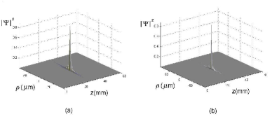
Figure 5: (a) The Frozen Wave with $Q=0.999\omega_{0}/c$ and $N=45$, approximately reproducing the chosen longitudinal pattern represented by eq.(77).  (b) A different Frozen wave, now with $Q=0.995\omega_{0}/c$ (but still with $N=45$) forwarding the same longitudinal pattern. We can observe that in this case (with a lower value for $Q$) a higher transverse localization is obtained.

With this, we can get some control on the transverse spot size through the parameter $Q$. Actually, eq.(74), which defines our FW, is a superposition of zero-order Bessel beams, and, due to this fact, the resulting field is expected to possess a transverse localization around $\rho=0$. Each Bessel beam in superposition (74) is associated with a central spot with transverse size, or width, $\Delta\rho_{m}\approx 2.4/k_{\rho\,m}$. On the basis of the expected convergence of series (74), we can estimate the width of the transverse spot of the resulting beam as being

$$\Delta\rho\approx\frac{2.4}{k_{\rho\,m=0}}\;=\;\frac{2.4}{\sqrt{\omega_{0}^{2}/c^{2}-Q^{2}}}\;,$$ (78)

which is the same value as that for the transverse spot of the Bessel beam with $m=0$ in superposition (74). Relation (78) can be useful: Once we have chosen the desired longitudinal intensity pattern, we can choose even the size of the transverse spot, and use relation (78) for evaluating the needed, corresponding value of parameter $Q$.

For a more detailed analyzis concerning the spatial resolution and residual intensity of the Frozen Waves, we refer the reader to ref.[17].

5.1.1 Increasing the control on the transverse shape by using higher-order Bessel beams

Here, we are going to argue that it is possible to increase even more our control on the transverse shape by using higher-order Bessel beams in our fundamental superposition (74).

This new approach can be understood and accepted on the basis of simple and intuitive arguments, which are not presented here, but can be found in ref.[17]. A brief description of that approach follows below.

The basic idea is obtaining the desired longitudinal intensity pattern not along the axis $\rho=0$, but on a cylindrical surface corresponding to $\rho=\rho^{\prime}>0$.

To do this, we first proceed as before: Once we have chosen the desired longitudinal intensity pattern $F(z)$, within the interval $0\leq z\leq L$, we calculate the coefficients $A_{m}$ as before, i.e.,  $A_{m}=(1/L)\int_{0}^{L}\,F(z)\,{\rm exp}(-i2\pi mz/L)\,{\rm d}z$, and $k_{\rho\,m}=\sqrt{\omega_{0}^{2}-\left(Q+2\pi m/L\right)^{2}}$.

Afterwards, we just replace the zero-order Bessel beams $J_{0}(k_{\rho\,m}\rho)$, in superposition (74), with higher-order Bessel beams, $J_{\mu}(k_{\rho\,m}\rho)$, to get

$${\Psi(\rho,z,t)\;=\;e^{-i\,\omega_{0}\,t}\,e^{i\,Q\,z}\,\sum_{m=-N}^{N}A_{m}\,J_{\mu}(k_{\rho\,m}\,\rho)\,e^{i\,\frac{2\pi}{L}m\,z}}\;,$$ (79)

With this, and based on intuitive arguments[17], we can expect that the desired longitudinal intensity pattern, initially constructed for $\rho=0$, will approximately shift to $\rho=\rho^{\prime}$, where $\rho^{\prime}$ represents the position of the first maximum of the Bessel function, i.e the first positive root of the equation  $({\rm d}\,J_{\mu}(k_{\rho\,m=0}\,\rho)/{\rm d}\rho)|_{\rho^{\prime}}=0$.

By such a procedure, one can obtain very interesting stationary configurations of field intensity, as “donuts”, cylindrical surfaces, and much more.

In the following example, we show how to obtain, e.g., a cylindrical surface of stationary light.  To get it, within the interval $0\leq z\leq L$, let us first select the longitudinal intensity pattern given by eq.(77), with $l_{1}=L/2-\Delta z$ and $l_{2}=L/2+\Delta z$, and with $\Delta z=L/300$. Moreover, let us choose $L=0.05\,$m, $Q=0.998\,\omega_{0}/c$, and use $N=150$.

Then, after calculating the coefficients $A_{m}$ by eq.(73), we have recourse to superposition (79). In this case, we choose $\mu=4$.  According to the previous discussion, one can expect the desired longitudinal intensity pattern to appear shifted to $\rho^{\prime}\approx 5.318/k_{\rho\,m=0}=8.47\,\mu$m, where 5.318 is the value of $k_{\rho\,m=0}\,\rho$ for which the Bessel function $J_{4}(k_{\rho\,m=0}\,\rho)$ assumes its maximum value, with $k_{\rho\,m=0}=\sqrt{\omega_{0}^{2}-Q^{2}}$.  The figure 6 below shows the resulting intensity field.

In Fig.6(a) the transverse section of the resulting beam for $z=L/2$ is shown. The transverse peak intensity is located at $\rho=7.75\,\mu$m, with a $8.5\%$ difference w.r.t. the predicted value of $8.47\,\mu$m. Figure 6(b) shows the orthogonal projection of the resulting field, which corresponds to nothing but a cylindrical surface of stationary light (or other fields).

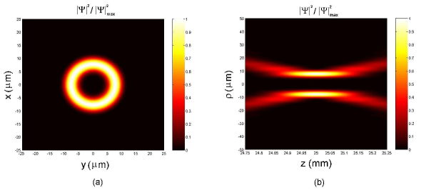
Figure 6: (a) Transverse section at $z=L/2$ of the considered higher-order FW.  (b) Orthogonal projection of the three-dimensional intensity pattern of the same higher-order FW.

We can see that the desired longitudinal intensity pattern has been approximately obtained, but, as wished, shifted from $\rho=0$ to $\rho=7.75\,\mu$m, and the resulting field resembles a cylindrical surface of stationary light with radius $7.75\,\mu$m and length $238\,\mu$m. Donut-like configurations of light (or sound) are also possible.

5.2 Stationary wavefields with arbitrary longitudinal shape in absorbing media: Extending the method.

When propagating in a non-absorbing medium, the so-called nondiffracting waves maintain their spatial shape for long distances. However, the situation is not the same when dealing with absorbing media. In such cases, both the ordinary and the nondiffracting beams (and pulses) will suffer the same effect: an exponential attenuation along the propagation axis.

Here, we are going to make an extension[10] of the method given above to show that, through suitable superpositions of equal-frequency Bessel beams, it is possible to obtain nondiffracting beams in absorbing media, whose longitudinal intensity pattern can assume any desired shape within a chosen interval $0\leq z\leq L$ of the propagation axis $z$.

As a particular example, we obtain new nondiffracting beams capable to resist the loss effects, maintaining amplitude and spot size of their central core for long distances.

It is important to stress that in this new method there is no active participation of the material medium. Actually, the energy absorption by the medium continues to occur normally, the difference being in the fact that these new beams have an initial transverse field distribution, such to be able to reconstruct (even in the presence of absorption) their central cores for distances considerably longer than the penetration depths of ordinary (nondiffracting or diffracting) beams. In this sense, the present method can be regarded as extending, for absorbing media, the self-reconstruction properties[27] that usual Localized Waves are known to possess in loss-less media.

In the same way as for lossless media, we construct a Bessel beam with angular frequency $\omega$ and axicon angle $\theta$ in the absorbing materials by superposing plane waves, with the same angular frequency $\omega$, and whose wave vectors lie on the surface of a cone with vertex angle $\theta$. The refractive index of the medium can be written as $n(\omega)=n_{R}(\omega)+in_{I}(\omega)$, quantity $n_{R}$ being the real part of the complex refraction index and $n_{I}$ the imaginary one, responsible for the absorbtion effects. With a plane wave, the penetration depth $\delta$ for the frequency $\omega$ is given by $\delta=1/\alpha=c/2\omega n_{I}$, where $\alpha$ is the absorption coefficient.

In this way, a zero-order Bessel beam in dissipative media can be written as  $\psi=J_{0}(k_{\rho}\rho){\rm exp}(i\beta z){\rm exp}(-i\omega t)$ with $\beta=n(\omega)\omega\cos\theta/c=n_{R}\omega\cos\theta/c+in_{I}\omega\cos\theta/c\equiv\beta_{R}+i\beta_{I}$; $k_{\rho}=n_{R}\omega\sin\theta/c+in_{I}\omega\sin\theta/c\equiv k_{\rho R}+ik_{\rho I}$, and so $k_{\rho}^{2}=n^{2}\omega^{2}/c^{2}-\beta^{2}$.  In this way,] it results   $\psi=J_{0}((k_{\rho R}+ik_{\rho I})\rho){\rm exp}(i\beta_{R}z){\rm exp}(-i\omega t){\rm exp}(-\beta_{I}z)$,   where $\beta_{R}$, $k_{\rho R}$ are the real parts of the longitudinal and transverse wave numbers, and $\beta_{I}$, $k_{\rho I}$ are the imaginary ones, while the absorption coefficient of a Bessel beam with axicon angle $\theta$ is given by $\alpha_{\theta}=2\beta_{I}=2n_{I}\omega\cos\theta/c$, its penetration depth being $\delta_{\theta}=1/\alpha_{\theta}=c/2\omega n_{I}\cos\theta$.

Due to the fact that $k_{\rho}$ is complex, the amplitude of the Bessel function $J_{0}(k_{\rho}\rho)$ starts decreasing from $\rho=0$ till the transverse distance $\rho=1/2k_{\rho I}$, and afterwards it starts growing exponentially. This behavior is not physically acceptable, but one must remember that it occurs only because of the fact that an ideal Bessel beam needs an infinite aperture to be generated. However, in any real situation, when a Bessel beam is generated by finite apertures, that exponential growth in the transverse direction, starting after $\rho=1/2k_{\rho I}$, will not occur indefinitely, stopping at a given value of $\rho$. Let us moreover emphasize that, when generated by a finite aperture of radius $R$, the truncated Bessel beam[17] possesses a depth of field $Z=R/\tan\theta$, and can be approximately described by the solution given in the previous paragraph, for $\rho<R$ and $z<Z$.

Experimentally, to guarantee that the mentioned exponential growth in the transverse direction does not even start, so as to meet only a decreasing transverse intensity, the radius $R$ of the aperture used for generating the Bessel beam should be $R\leq 1/2k_{\rho I}$. However, as noted by Durnin et al., the same aperture has to satisfy also the relation $R\geq 2\pi/k_{\rho R}$. From these two conditions, we can infer that, in an absorbing medium, a Bessel beam with just a decreasing transverse intensity can be generated only when the absorption coefficient is $\alpha<2/\lambda$, i.e., if the penetration depth is $\delta>\lambda/2$. The method developed in this paper does refer to these cases, i.e. we can always choose a suitable finite aperture size in such a way that the truncated versions of all solutions presented in this work, including the general one given by eq.(6), will not present any unphysical behavior. Let us now outline our method.

Consider an absorbing medium with the complex refraction index $n(\omega)=n_{R}(\omega)+in_{I}(\omega)$, and the following superposition of $2N+1$ Bessel beams with the same frequency $\omega$:

$$\begin{array}[]{clr}\Psi(\rho,z,t)=\displaystyle{\sum_{m=-N}^{N}}A_{m}\,J_{0}\left((k_{\rho R_{m}}+ik_{\rho I_{m}})\rho\right)\,e^{i\,\beta_{R_{m}}z}\,e^{-i\,\omega\,t}\,e^{-\beta_{I_{m}}z}\;,\end{array}$$ (80)

where the $m$ are integer numbers, the $A_{m}$ are constant (yet unknown) coefficients, quantities $\beta_{R_{m}}$ and $k_{\rho R_{m}}$ ($\beta_{I_{m}}$ and $k_{\rho I_{m}}$) are the real (the imaginary) parts of the complex longitudinal and transverse wave numbers of the $m$-th Bessel beam in superposition (80); the following relations being satisfied

$$k_{\rho_{m}}^{2}\;=\;n^{2}\frac{\omega^{2}}{c^{2}}-\beta_{m}^{2}$$ (81)

$$\frac{\beta_{R_{m}}}{\beta_{I_{m}}}\;=\;\frac{n_{R}}{n_{I}}$$ (82)

where $\beta_{m}=\beta_{R_{m}}+i\beta_{I_{m}}$, $k_{\rho_{m}}=k_{\rho R_{m}}+ik_{\rho I_{m}}$, with $k_{\rho R_{m}}/k_{\rho I_{m}}=n_{R}/n_{I}$.

Our goal is now to find out the values of the longitudinal wave numbers $\beta_{m}$ and the coefficients $A_{m}$ in order to reproduce approximately, inside the interval $0\leq z\leq L$ (on the axis $\rho=0$), a freely chosen longitudinal intensity pattern that we call $|F(z)|^{2}$.

The problem for the particular case of lossless media[16,17], i.e., when $n_{I}=0\rightarrow\beta_{I_{m}}=0$, was solved in the previous subsection. For those cases, it was shown that the choice $\beta=Q+2\pi m/L$, with $A_{m}=\int_{0}^{L}F(z){\rm exp}(-i2\pi mz/L)/L\,\,dz$ can be used to provide approximately the desired longitudinal intensity pattern $|F(z)|^{2}$ on the propagation axis, within the interval $0\leq z\leq L$, and, at the same time, to regulate the spot size of the resulting beam by means of the parameter $Q$, which parameter can be also used to obtain large field depths and also to inforce the linear polarization approximation to the electric field for the TE electromagnetic wave (see details in refs.[16,17]).

However, when dealing with absorbing media, the procedure described in the last paragraph does not work, due to the presence of the functions ${\rm exp}(-\beta_{I_{m}}z)$ in the superposition (80), since in this case that series does not became a Fourier series when $\rho=0$.

On attempting to overcome this limitation, let us write the real part of the longitudinal wave number, in superposition (80), as

$$\beta_{R_{m}}\;=\;Q+\frac{2\pi m}{L}$$ (83)

with

$$0\leq Q+\frac{2\pi m}{L}\leq n_{R}\frac{\omega}{c}$$ (84)

where this inequality guarantees forward propagation only, with no evanescent waves.

In this way the superposition (80) can be written

$$\begin{array}[]{clr}\Psi(\rho,z,t)=e^{-i\,\omega\,t}\,e^{i\,Qz}\,\displaystyle{\sum_{m=-N}^{N}}A_{m}\,J_{0}\left((k_{\rho R_{m}}+ik_{\rho I_{m}})\rho\right)\,e^{i\,\frac{2\pi m}{L}z}\,e^{-\beta_{I_{m}}z}\;,\end{array}$$ (85)

where, by using (82), we have $\beta_{I_{m}}=(Q+2\pi m/L)n_{I}/n_{R}$, and $k_{\rho_{m}}=k_{\rho R_{m}}+ik_{\rho I_{m}}$ is given by (81). Obviously, the discrete superposition (85) could be written as a continuous one (i.e., as an integral over $\beta_{R_{m}}$) by taking $L\rightarrow\infty$, but we prefer the discrete sum due to the difficulty of obtaining closed-form solutions to the integral form.

Now, let us examine the imaginary part of the longitudinal wave numbers. The minimum and maximum values among the $\beta_{I_{m}}$ are $(\beta_{I})_{\rm min}=(Q-2\pi N/L)n_{I}/n_{R}$ and $(\beta_{I})_{\rm max}=(Q+2\pi N/L)n_{I}/n_{R}$, the central one being given by $\overline{\beta}_{I}\equiv(\beta_{I})_{m=0}=Qn_{I}/n_{R}$. With this in mind, let us evaluate the ratio $\Delta=[(\beta_{I})_{\rm max}-(\beta_{I})_{\rm min}]/{\overline{\beta}_{I}}=4\pi N/LQ$.

Thus, when $\Delta<<1$, there are no considerable differences among the various $\beta_{I_{m}}$, since $\beta_{I_{m}}\approx\overline{\beta}_{I}$ holds for all $m$. In the same way, there are no considerable differences among the exponential attenuation factors, since ${\rm exp}(-\beta_{I_{m}}z)\approx{\rm exp}(-\overline{\beta}_{I}z)$. So, when $\rho=0$ the series in the r.h.s. of eq.(85) can be approximately considered a truncated Fourier series multiplied by the function ${\rm exp}(-\overline{\beta}_{I}z)$ and, therefore, superposition (85) can be used to reproduce approximately the desired longitudinal intensity pattern $|F(z)|^{2}$ (on $\rho=0$), within $0\leq z\leq L$, when the coefficients $A_{m}$ are given by

$$A_{m}\;=\;\frac{1}{L}\,\int_{0}^{L}F(z)\,e^{\overline{\beta}_{I}z}e^{-i\,\frac{2\pi m}{L}z}\,dz,$$ (86)

being necessary the presence of the of the factor ${\rm exp}(\overline{\beta}_{I}z)$ in the integrand to compensate for the factors ${\rm exp}(-\beta_{I_{m}}z)$ in superposition (85).

Since we are adding together zero-order Bessel functions, we can expect a good field concentration around $\rho=0$.

In short, we have shown in this Section how one can get, in an absorbing medium, a stationary wave-field with a good transverse concentration, and whose longitudinal intensity pattern (on $\rho=0$) can approximately assume any desired shape $|F(z)|^{2}$ within the predetermined interval $0\leq z\leq L$. The method is a generalization of a previous one[16,17] and consists in the superposition of Bessel beams in EQ.(85), the real and imaginary parts of their longitudinal wave numbers being given by eqs.(83)and (82), while their complex transverse wave numbers are given by eq.(81), and, finally, the coefficients of the superposition are given by eq.(86). The method is justified, since $4\pi N/LQ<<1$; happily enough, this condition is satisfied in a great number of situations.

Regarding the generation of these new beams, given an apparatus capable of generating a single Bessel beam, we can use an array of such apparatuses to generate a sum of them, with the appropriate longitudinal wave numbers and amplitudes/phases [as required by the method], thus producing the desired beam. For instance, we can use[16,17] a laser illuminating an array of concentric annular apertures (located at the focus of a convergent lens) with the appropriate radii and transfer functions, able to yield both the correct longitudinal wave numbers (once a value for $Q$ has been chosen) and the coefficients $A_{n}$ of the fundamental superposition (85).

5.2.1 Some Examples

For generality’s sake, let us consider a hypothetical medium in which a typical XeCl excimer laser ($\lambda=308{\rm nm}\rightarrow\omega=6.12\times 10^{15}$Hz) has a penetration depth of 5 cm; i.e. an absorption coefficient $\alpha=20{\rm m}^{-1}$, and therefore $n_{I}=0.49\times 10^{-6}$. Besides this, let us suppose that the real part of the refraction index for this wavelength is $n_{R}=1.5$ and therefore $n=n_{R}+in_{I}=1.5+i\,0.49\times 10^{-6}$. Note that the value of the real part of the refractive index is not so important for us, since we are dealing with monochromatic wave fields.

A Bessel beam with $\omega=6.12\times 10^{15}$Hz and with an axicon angle $\theta=0.0141\;$rad (so, with a transverse spot of radius $8.4\,\mu$m), when generated by an aperture, say, of radius $R=3.5\;$mm, can propagate in vacuum a distance equal to $Z=R/\tan\theta=25\;$cm while resisting the diffraction effects. However, in the material medium considered here, the penetration depth of this Bessel beam would be only $z_{p}=5\;$cm. Now, let us set forth two interesting applications of the method.

First Example: Almost Undistorted Beams in Absorbing Media.

Now, we can use the extended method to obtain, in the same medium and for the same wavelength, an almost undistorted beam capable of preserving its spot size and the intensity of its central core for a distance many times larger than the typical penetration depth of an ordinary beam (nondiffracting or not).

With this purpose, let us suppose that, for this material medium, we wish a beam (with $\omega=6.12\times 10^{15}$Hz) that maintains amplitude and spot size of its central core for a distance of $25\;$cm, i.e. a distance 5 times greater than the penetration depth of an ordinary beam with the same frequency. We can model this beam by choosing the desired longitudinal intensity pattern $|F(z)|^{2}$ (on $\rho=0$), within $0\leq z\leq L$,

$$F(z)\;=\;\left\{\begin{array}[]{clr}&1\;\;\;{\rm for}\;\;\;0\leq z\leq Z\\ &0\;\;\;\mbox{elsewhere},\end{array}\right.$$ (87)

and by putting $Z=25\;$cm, with, for example, $L=33\;$cm.

Now, the Bessel beam superposition (85) can be used to reproduce approximately this intensity pattern, and to this purpose let us choose $Q=0.9999\omega/c$ for the $\beta_{R_{m}}$ in (83), and $N=20$ (note that, according to inequality (84), $N$ could assume a maximum value of $158$.)

Once we have chosen the values of $Q$, $L$ and $N$, the values of the complex longitudinal and transverse Bessel beams wave numbers happen to be defined by relations (83), (82) and (81). Eventually, we can use eq.(86) and find out the coefficients $A_{m}$ of the fundamental superposition (85), that defines the resulting stationary wave-field.

Let us just note that the condition $4\pi N/LQ<<1$ is perfectly satisfied in this case.

In Fig. (7)(a) we can see the 3D field-intensity of the resulting beam. One can see that the field possesses a good transverse localization (with a spot size smaller than $10\;\mu$m), it being capable of maintaining spot size and intensity of its central core till the desired distance (a better result could be reached by using a higher value of $N$).

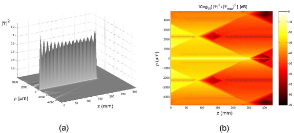
Figure 7: (a) Three-dimensional field-intensity of the resulting beam. (b) The resulting beam, in an orthogonal projection and in logaritmic scale.

It is interesting to note that at this distance (25 cm), an ordinary beam would have got its initial field-intensity attenuated $148$ times.

As we have said in the Introduction, the energy absorption by the medium continues to occur normally; the difference is that these new beams have an initial transverse field distribution sophisticated enough to be able to reconstruct (even in the presence of absorption) their central cores till a certain distance. For a better visualization of this field-intensity distribution and of the energy flux, Fig.(7)(b) shows the resulting beam, in an orthogonal projection and in logarithmic scale. It is clear that the energy comes from the lateral regions, in order to reconstruct the central core of the beam. On the plane $z=0$, within the region $\rho\leq R=3.5\,$mm, there is a uncommon field intensity distribution, being very dispersed instead of concentrated. This uncommon initial field intensity distribution is responsible for constructing the central core of the resulting beam and for its reconstruction till the distance $z=25\,$cm. Due to absorption, the beam (total) energy flowing through different $z$ planes, is not constant, but the energy flowing IN the beam spot area and the beam spot size itself are conserved till (in this case) the distance $z=25\,$ cm.

Second Example: Beams in absorbing media with a growing longitudinal field intensity.

Considering again the previous hypothetical medium, in which an ordinary Bessel beam with $\theta=0.0141\;$rad and $\omega=6.12\times 10^{15}$Hz has a penetration depth of $5\;$cm, we aim to construct now a beam that, instead of possessing a constant core-intensity till the position $z=25\;$cm, presents on the contrary a (moderate) exponential growth of its intensity, till that distance ($z=25\;$cm).

Let us assume we wish to get the longitudinal intensity pattern $|F(z)|^{2}$, in the interval $0<z<L$,

$$F(z)\;=\;\left\{\begin{array}[]{clr}&{\rm exp}(z/Z)\;\;\;{\rm for}\;\;\;0\leq z\leq Z\\ &0\;\;\;\mbox{elsewhere},\end{array}\right.$$ (88)

with $Z=25\,$cm and $L=33\;$cm.

Using again $Q=0.9999\omega/c$, $N=20$, we CAN proceed as in the first example, calculating the complex longitudinal and transverse Bessel beams wave numbers and finally the coefficients $A_{m}$ of the fundamental superposition (85).

In Fig. (8) we can see the 3D field-intensity of the resulting beam. One can see that the field presents the desired longitudinal intensity pattern with a good transverse localization (a spot size smaller than $10\;\mu$m).

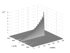
Figure 8: Three-dimensional field-intensity of the resulting beam, in an absorbing medium, with a growing longitudinal field intensity.

Obviously, the amount of energy necessary to construct these new beams is greater than that necessary to generate an ordinary beam in a non-absorbing medium. And it is also clear that there is a limitation on the depth of field of these new beams. In the first example, for distances longer than 10 times the penetration depth of an ordinary beam, besides a greater energy demand, we meet the fact that the field-intensity in the lateral regions would be even higher than that of the core, and the field would loose the usual characteristics of a beam (transverse field concentration)

References

[1] A much more complete list of references can be found in the previous chapter (Chapter 1) of this book, that is, of Localized Waves, ed. by H.E.Hernández-Figueroa, M.Zamboni-Rached and E.Recami (J.Wiley; in press).

[2] J. N. Brittingham, “Focus wave modes in homogeneous Maxwell’s equations: transverse electric mode,” J. Appl. Phys., Vol. 54, pp. 1179-1189 (1983).

[3] J. Durnin, J. J. Miceli e J. H. Eberly, “Diffraction-free beams,” Phys. Rev. Lett., Vol. 58, pp. 1499-1501 (1987).

[4] J.-y. Lu, J. F. Greenleaf, “Nondiffracting X-waves - Exact solutions to free-space wave equation and their finite aperture realizations,” IEEE Transactions in Ultrasonics Ferroelectricity and Frequency Control, Vol.39, pp.19-31 (1992); and refs. therein.

[5] H.Sõnajalg, P.Saari, “Suppression of temporal spread of ultrashort pulses in dispersive media by Bessel beam generators”, Opt. Letters, Vol. 21, pp.1162-1164 (1996).

[6] M. Zamboni-Rached, K. Z. Nóbrega, H. E. Hern’ndez-Figueroa e E. Recami, “Localized Superluminal solutions to the wave equation in (vacuum or) dispersive media, for arbitrary frequencies and with adjustable bandwidth”, Optics Communications, Vol.226, pp. 15-23 (2003).

[7] M.A.Porras, R.Borghi, and M.Santarsiero, “Suppression of dispersion broadening of light pulses with Bessel-Gauss beams”, Optics Communications, Vol. 206, 235-241 (2003).

[8] C.Conti, S.Trillo, P.Di Trapani, G.Valiulis, A.Piskarskas, O.Jedrkiewicz and J.Trull, “Nonlinear electromagnetic X-waves”, Phys. Rev. Lett., vol.90, paper no.170406, May 2003; and refs. therein.

[9] J. Salo, J. Fagerholm, A. T. Friberg, and M. M. Salomaa, “Nondiffracting Bulk-Acoustic X waves in Crystals,” Phys. Rev. Lett., Vol. 83, pp. 1171-1174 (1999); and refs. therein.

[10] M. Zamboni-Rached, ”Diffraction-Attenuation resistant beams in absorbing media”, Optics Express, Vol. 14, pp.1804-1809 (2006).

[11] I. M. Besieris, A. M. Shaarawi e R. W. Ziolkowski, “A bidirectional traveling plane wave representation of exact solutions of the scalar wave equation”, J. Math. Phys., Vol. 30, pp. 1254-1269 (1989).

[12] M. Zamboni-Rached, “ Localized Waves: Structure and Applications,” M.Sc. Thesis (Physics Department, Unicamp, 1999).

[13] M. Zamboni-Rached, E. Recami, H. E. Hernández-Figueroa, ”New localized Superluminal solutions to the wave equations-with finite total energies and arbitrary frequencies”, European Physics Journal D, Vol. 21, 217-228 (2002).

[14] M.Zamboni-Rached, “Localized waves in diffractive/dispersive media”, PhD Thesis, Aug.2004, Universidade Estadual de Campinas, DMO/FEEC. Download at:

http://libdigi.unicamp.br/document/?code=vtls000337794

[15] S. Longhi, “Localized subluminal envelope pulses in dispersive media,” Optics Letters, Vol. 29, pp.147-149 (2004);and refs. therein.

[16] M. Zamboni-Rached, “Stationary optical wave fields with arbitrary longitudinal shape by superposing equal frequency Bessel beams: Frozen Waves”, Optics Express, Vol. 12, pp.4001-4006 (2004).

[17] M. Zamboni-Rached, E. Recami, H. E. Hernández-Figueroa, “Theory of Frozen Waves: Modelling the Shape of Stationary Wave Fields”, Journal of Optical Society of America A, Vol. 22, pp.2465-2475.

[18] S. V. Kukhlevsky and M. Mechler, “Diffraction-free subwavelength-beam optics at nanometer scale,” Optics Communications, Vol. 231, pp.35-43 (2004).

[19] I.S.Gradshteyn, and I.M.Ryzhik: Integrals, Series and Products, 4th edition (Acad. Press; New York, 1965).

[20] A.M.Shaarawi, I.M.Besieris and T.M.Said, “Temporal focusing by use of composite X-waves”, J. Opt. Soc. Am., A, vol.20, pp.1658-1665, Aug.2003.

[21] M. Zamboni-Rached, A. Shaarawi, E. Recami, “Focused X-Shaped Pulses”, Journal of Optical Society of America A, Vol. 21, pp. 1564-1574 (2004).

[22] M. Zamboni-Rached, H.E. Hernández-Figueroa, E. Recami “Chirped Optical X-type Pulses,” Journal of Optical Society of America A, Vol. 21, pp. 2455-2463 (2004).

[23] G. Agrawal: Nonlinear Fiber Optics (Academic Press; 4th edition, 2006).

[24] Z. Bouchal and M. Olivik, “‘Non-diffractive vector Bessel beams,” Journal of Modern Optics, Vol. 42, pp.1555-1566 (1995).

[25] E.Recami: “On localized X-shaped Superluminal solutions to Maxwell equations,” Physica A, Vol. 252, pp.586-610 (1998).

[26] Z. Bouchal, “Controlled spatial shaping of nondiffracting patterns and arrays”, Optics Letters, Vol. 27, pp. 1376-1378 (2002).

[27] R. Grunwald, U. Griebner, U. Neumann, and V. Kebbel, Self-reconstruction of ultrashort-pulse Bessel-like X-waves, CLEO / QELS 2004, San Francisco, May 16-21, 2004, Conference Digest (CD-ROM), paper number CMQ7.