DLAs and Galaxy Formation

Abstract

Damped Lyman-$\alpha$ systems (DLAs) are useful probes of star formation and galaxy formation at high-redshift (hereafter high-$z$). We study the physical properties of DLAs and their relationship to Lyman break galaxies (LBGs) using cosmological hydrodynamic simulations based on the concordance $\Lambda$ cold dark matter model. Fundamental statistics such as global neutral hydrogen (H i) mass density, H i column density distribution function, DLA rate-of-incidence and mean halo mass of DLAs are reproduced reasonably well by the simulations, but with some deviations that need to be understood better in the future. We discuss the feedback effects by supernovae and galactic winds on the DLA distribution. We also compute the [C ii] emission from neutral gas in high-$z$ galaxies, and make predictions for the future observations by the Atacama Large Millimeter Array (ALMA) and Space Infrared Telescope for Cosmology and Astrophysics (SPICA). Agreement and disagreement between simulations and observations are discussed, as well as the future directions of our DLA research.

Received (Day Month Year)Revised (Day Month Year)

1 Introduction

Recent studies suggest that our universe can be described well by a cosmological model called the concordance $\Lambda$ cold dark matter (CDM) model with a matter energy density $\Omega_{\rm m}\equiv\rho_{\rm m}/\rho_{\rm crit}\simeq 0.3$ and a dark energy density $\Omega_{\Lambda}\equiv\rho_{\Lambda}/\rho_{\rm crit}\simeq 0.7$. [1, 2, 3] Based on this backbone of structure formation, we would like to build a self-consistent model of galaxy formation that can describe the formation of disk, spheroid, and black holes. In particular, we would like to understand how the gas turned into stars as a function of cosmic time and environment.

Observations of DLAs provide very unique opportunities for that purpose. Because DLAs are observed in absorption, they are in principle an unbiased sample of H i in the universe, and provide us with information that are complementary to those obtained by direct observations of stellar emission. For example, with DLAs we can measure the global H i mass density in the universe as a function of redshift.[6] It has been estimated that DLAs contain a significant fraction of H i gas in the universe at $z\sim 3$, with the amount roughly equal to a half of current stellar mass density. [7, 8, 9, 10] Therefore DLAs are considered to be important reservoirs of neutral gas for star formation in high-$z$ universe, and their study would reveal the physical properties of neutral gas before they turn into stars. The conversion history of neutral gas into stars has been an active area of research over the past ten years, [11, 12, 13, 14, 15, 16] and the connection between DLAs and star-forming galaxies such as LBGs[12] is becoming one of the focus of current DLA research.

In recent years, observers have made significant progress in constraining the statistical properties of DLAs using large samples of high-$z$ quasars discovered by surveys such as the Sloan Digital Sky Survey (SDSS)[17]. For example, Ref. Pro05 have extracted $\approx 500$ DLAs from the SDSS Data Release 3 and tightened the constraints on the column density distribution function and the rate of incidence. The total number of detected DLAs has reached over 1000 as of early 2007 (Prochaska, private communication). Increased accuracy in these observables set tight constraints on the models of galaxy formation.

In turn, theoretical understanding of DLAs remain unsatisfactory. Currently there are mainly two competing views on the physical origin of DLAs. One idea is that DLAs originate from rapidly rotating, massive disk galaxies.[18] This model can explain the large velocity widths of low-ionization metal absorption lines. However, Ref. Hae98 used hydrodynamic simulations to argue that the asymmetric profiles of low-ionization absorption lines can also be explained by the rotation, random motions, infall, and merging of protogalactic gas clumps equally well. Somewhat intermediate idea is intersecting multiple disks [20] or tidal tails observed in merging systems.

There are a number of DLA studies using so-called semianalytic models of galaxy formation[21, 22], but it would also be desirable to study DLAs using cosmological hydrodynamic simulations that directly solve the gas dynamics within the framework of $\Lambda$CDM universe. Ref. NSH04a & NSH04b focused on the effects of star formation and supernova (SN) feedback on DLAs that were largely neglected by the earlier numerical work, [25, 26, 27] and showed that the distribution of DLAs could be significantly affected by SN feedback. Ref. Razoumov06a studied the effects of radiative transfer by post-processing the results of cosmological hydrodynamic simulations, but their simulations did not include models for star formation and SN feedback. It is still difficult to treat the radiative transfer dynamically from all galaxies in a large volume of space, as well as star formation and feedback by SNe and active galactic nuclei in large-scale cosmological hydrodynamic simulations. This is primarily due to the heavy computational load required for such a simulation with full treatment of all physical processes. At the moment, we need to limit our calculation to a small number of objects in order to treat radiative transfer self-consistently with the star formation in simulations.

In this review article, we summarize our recent numerical studies on DLAs using cosmological hydrodynamic simulations. We discuss the conflicts and agreement between simulations and observations, and the future directions of theoretical research on DLAs.

2 Simulating DLAs

We use cosmological smoothed particle hydrodynamics (SPH) code GADGET-2 (Springel 2005) for our study. The code solves the hydrodynamics in a Lagrangian fashion by allowing the gas particles to cluster in high density regions, thereby providing higher resolution in galaxy-forming regions. The gravity is solved by a Tree-particle-mesh method that uses a tree algorithm for the short-range force and particle-mesh technique for the long-range force. It also adopts the entropy-conservative formulation[29] to remedy the overcooling problem, which previous generation of cosmological SPH codes suffered from. The code includes radiative cooling, heating by a uniform UV background radiation of a modified Haardt & Madau spectrum[30, 31, 32], star formation, supernova feedback, galactic wind[33], and a sub-resolution multiphase model of interstellar medium (ISM)[34].

We employ a series of simulations with different resolution, box sizes (from ${\rm L_{box}}=4h^{-1}{\rm\,Mpc}$ to $100h^{-1}{\rm\,Mpc}$) and feedback strengths to study their effects. One of the focus of our study is to examine the effects of galactic wind feedback on the distribution of DLAs. In this article, we summarize our results by referring to two cases: ‘no wind’ feedback and ‘strong wind’ feedback, corresponding to the wind speed of $v_{w}=0$ and 484 km s^-1. See Ref. NSH04b for more details of our simulations. All of our simulations are based on a concordance $\Lambda$CDM cosmology with cosmological parameters $(\Omega_{\rm m},\Omega_{\Lambda},\Omega_{\rm b},\sigma_{8},h)=(0.3,0.7,0.04,0.9,0.7)$, where $h=H_{0}/(100\,\rm km\,s^{-1}\,Mpc^{-1})$.

3 Fundamental DLA Statistics

3.1 H I Column Density Distribution

The H i column density distribution function $f(N_{\rm HI})$ is the most fundamental statistic for any H i quasar absorption systems. It counts the number of columns in bins of [$N_{\rm HI},N_{\rm HI}+dN_{\rm HI}$] per unit absorption distance $dX$, i.e., $dN=f(N_{\rm HI})dN_{\rm HI}dX$, where $dX\equiv\frac{H_{0}}{c}(1+z)^{3}\,c\,dt=\frac{H_{0}}{c}\,(1+z)^{2}\,dr$. The quantity $dN$ can also be interpreted as an area covering fraction in the sky along the line element $c\,dt$.

Ref. NSH04a examined $f(N_{\rm HI})$ in a series of cosmological SPH simulations with different box sizes and resolution. The left panel of Fig. 1 shows the results for runs with no wind and strong wind feedback, together with the observed data points.[9] At high column densities ($\log N_{\rm HI}>21$), the agreement between the strong feedback run and observed data is quite good. The run with no wind feedback significantly overpredicts $f(N_{\rm HI})$. This is because the galactic wind feedback reduces the number of columns with large $N_{\rm HI}$ by ejecting the gas from star-forming regions and heat the H i gas. This agreement at $\log N_{\rm HI}>21$ for the strong feedback run is encouraging and shows the effectiveness of our current wind feedback model. One might speculate that the H i in the overpredicted columns in the no feedback run could turn into molecular hydrogen, therefore the apparent disagreement between the simulation and the data points is not a serious problem. However, Ref. Zwaan06 showed that the H₂ column density distribution forms a natural extension to $f(N_{\rm HI})$ for local galaxies, and that the connection point between the two distribution is at $(\log N_{\rm HI},\log f(N_{\rm HI}))\approx(22,-26)$. Since the degree of overprediction in the no feedback run is more than a factor of 2 at $\log N_{\rm HI}\lesssim 22$, it seems difficult to hide all of the overpredicted H i in the form of H₂ if similar atomic and molecular physics hold in high-$z$ galaxies as in local galaxies.

Our simulations underpredict the number of columns with $20<\log N_{\rm HI}<21$ regardless of the strength of wind feedback. Physical reasons for this underestimate is not clear at this point. Several test runs show that this feature does not change very much with varying threshold density or time-scale for star formation, or varying wind feedback strength. Any combination of the following could be the cause for this underestimate: inadequate resolution, angular momentum transfer problem, inadequate cooling due to lack of metal cooling in the current code, too simplistic models for star formation and SN feedback, or poor treatment of radiative transfer. We plan to address these issues in our future work.

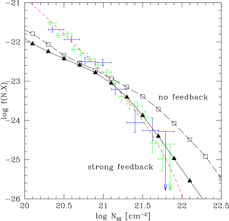
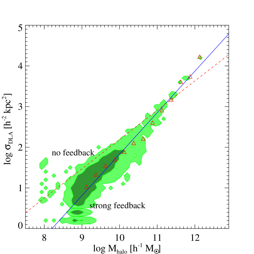
Figure 1: Left: Column density distribution function $f(N_{\rm HI})$ for the runs with no wind (open squares) and strong wind feedback (solid triangles). The red short-dashed line is the gamma function fit to the observed data points[9]. Right: Comoving DLA cross section as a function of halo mass. The shaded contours show the distribution of halos for the run with strong wind feedback. The open triangle symbols are the median points in each mass bin, and the solid line is the least-square fit to the median points. The dashed line is the same fit for the run with no wind feedback.

3.2 Neutral Gas Mass Density

For a given observed path length $c\Delta t$, the H i mass density within the survey volume can be estimated as follows (in proper units):

$$\rho_{\rm HI}=\frac{m_{\rm H}}{c\Delta t}\int_{N_{\rm min}}^{N_{\rm max}}N_{\rm HI}f(N_{\rm HI})dN_{\rm HI}\Delta X=\frac{H_{0}m_{\rm H}(1+z)^{3}}{c}\int_{N_{\rm min}}^{N_{\rm max}}N_{\rm HI}f(N_{\rm HI})dN_{\rm HI},$$ (1)

where $m_{H}$ is the mass of a hydrogen atom, and $[N_{\rm min},N_{\rm max}]$ is the observed range of $N_{\rm HI}$. If the observed range of $N_{\rm HI}$ is broad enough and covers up to sufficiently high $N_{\rm HI}$ values, then one can expect that the calculated quantity is representative of the true value in the universe, and the mass density parameter of neutral gas can be estimated as $\Omega_{\rm neutral}=\mu\rho_{\rm HI}/\rho_{\rm crit}$, where $\mu\approx 1.3$ is inserted to take helium into account. It is known observationally[7, 8, 9] that DLAs dominate the H i mass density at $z\sim 3$, with the amount roughly equal to half of the present-day stellar mass density. This suggests that DLAs are important reservoirs of neutral gas for star formation in high-$z$ galaxies, and that the neutral gas in DLAs at $z=3$ are converted into stars between $z=3$ and $z=0$. Ref. NSH04a showed that the observed estimates of $\Omega_{\rm neutral}$ can be bracketed by the simulation with no wind and strong wind feedback. It can also be shown that high-$N_{\rm HI}$ systems dominate $\Omega_{\rm HI}$, therefore it is important to include a fair number of high-$N_{\rm HI}$ systems in the sample to obtain an accurate fit to $f(N_{\rm HI})$ and estimate $\Omega_{\rm HI}$ reliably.

3.3 DLA Cross Section vs. Halo Mass

It is useful to quantify the cross section of DLAs ($\sigma_{\rm DLA}$) as a function of dark matter halo mass, because we have a theoretical framework to compute the halo mass function. [36, 37] Observers can identify DLAs only in the quasar sight-lines, but there could be multiple neutral gas clouds within the same halo that do not cross the quasar sight-line. Therefore it is theoretically more plausible to characterize the occurrence of DLAs as a cross section rather than the number of clouds in each halo.

Ref. NSH04a estimated the relationship between the total DLA cross section $\sigma_{\rm DLA}^{co}$ (in units of comoving $h^{-2}$ kpc²) and the dark matter halo mass (in units of $h^{-1}{\rm M_{\odot}}$) at $z=3$ as

$$\log\,\sigma_{\rm DLA}^{co}=\alpha\,(\log\,M_{\rm halo}-12)+\beta,$$ (2)

with slopes $\alpha=0.7-1.0$ and normalization $\beta=3.9-4.2$, depending on the numerical resolution and the strength of galactic wind feedback. The slope $\alpha$ is always positive and massive halos have larger DLA cross sections, but they are more scarce compared to less massive halos. Two important features are: (1) As the strength of galactic wind feedback increases, the slope $\alpha$ become steeper while the normalization $\beta$ remains roughly constant. This is because a stronger wind reduces the amount of neutral gas in low-mass halos at a higher rate by ejecting the gas out of the potential well of the halo. (2) As the numerical resolution is improved, both the slope and the normalization increase. This is because with higher resolution, simulations can resolve higher densities, and star formation in low-mass halos can be described better. As a result the neutral gas content is decreased due to winds. On the other hand, a lower resolution run misses the early generation of halos and the neutral gas in them, resulting in lower $\Omega_{\rm HI}$ at high-$z$.

Earlier numerical work[25, 26, 27] largely neglected the effects of star formation and wind feedback, therefore they often overestimated the DLA cross sections in low-mass halos, resulting in higher value of predicted rate-of-incidence (see § 3.4). In order to match their results with observed data, they introduced a minimum halo mass that DLAs populate. Our simulations show that star formation and feedback affect the DLA distribution, therefore, we need to study their effects further with better resolution and improved models of star formation and feedback.

3.4 DLA Rate-of-Incidence

The probability of finding a DLA for a given observed path-length can be expressed as a rate-of-incidence. Theoretically, we can compute the cumulative rate-of-incidence of DLAs per unit redshift above certain minimum halo mass $M$ as

$$\frac{{\rm d}N_{\rm DLA}}{{\rm d}z}(>M)=\frac{{\rm d}r}{{\rm d}z}\int_{M}^{\infty}n_{\rm dm}(M^{\prime})~{}\sigma_{\rm DLA}^{co}(M^{\prime})\,{\rm d}M^{\prime},$$ (3)

where $n_{\rm dm}(M)$ is the dark matter halo mass function and ${\rm d}r/{\rm d}z=c/H(z)$ with $H(z)=H_{0}\sqrt{\Omega_{\rm m}(1+z)^{3}+\Omega_{\Lambda}}$ for a flat universe. In order to carry out this integral, Eq. (2) can be used.

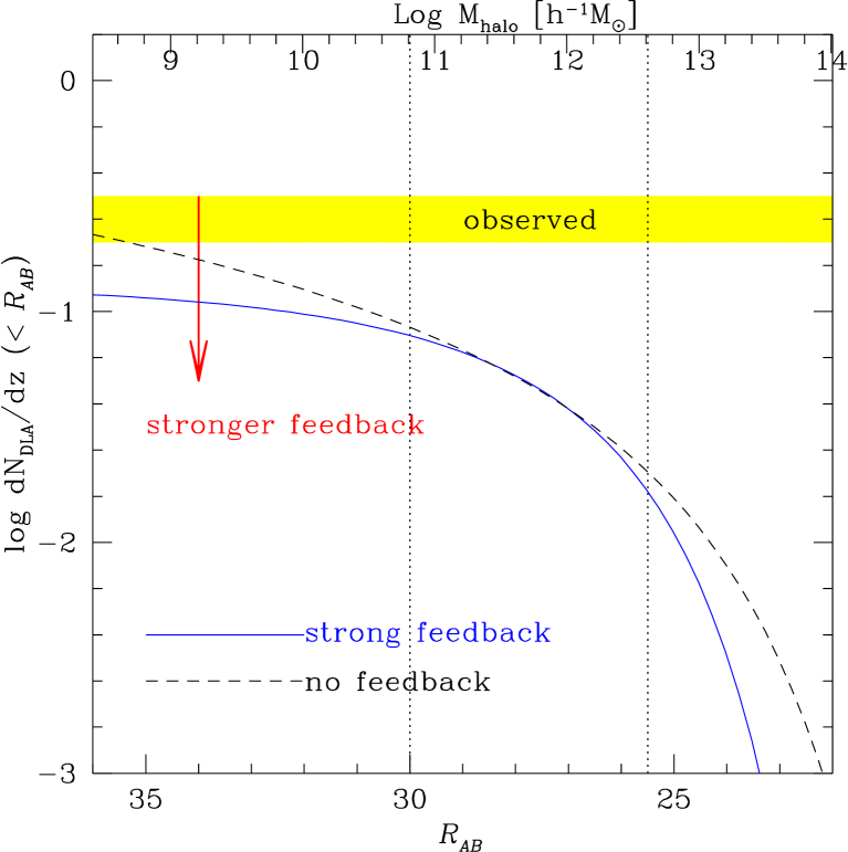
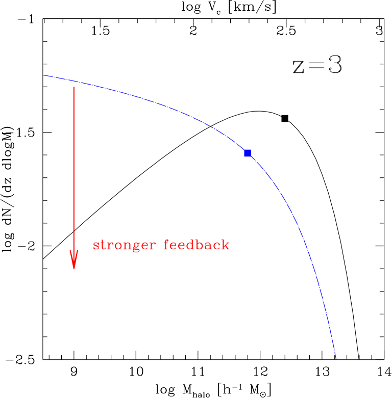
Figure 2: Left: Cumulative DLA rate-of-incidence for all galaxies above certain magnitude limit. An observational estimate[9] is shown by the hatched band. Right: Probability distribution function of DLA rate-of-incidence as a function of dark matter halo mass. As the feedback strength increases, contribution from low-mass halos decreases, and the distribution shifts toward higher masses with a peak emerging at $M_{\rm halo}\simeq 10^{12}h^{-1}{\rm M_{\odot}}$.

The left panel of Fig. 2 shows that the run with no wind feedback agrees with the observed rate if we sample the halos down to $M_{\rm halo}\simeq 10^{8.5}h^{-1}{\rm M_{\odot}}$. The run with strong feedback underestimates the total DLA rate-of-incidence by about 0.3 dex due to the underestimate of $f(N_{\rm HI})$ at $\log N_{\rm HI}<21$. Based on the results of hydro simulations, Ref. Nag07 derived the mean scaling relation between halo mass and galaxy $R$-band AB magnitude as

$$R_{AB}=-2.5\log M_{\rm halo}+C-5\log h_{70},$$ (4)

where $C=55.03$ (no feedback) and $57.03$ (strong feedback). This relation was used to convert the halo mass into apparent $R_{AB}$ magnitude in the left panel of Fig. 2. The arrows in the figure indicate that the wind feedback reduces the contribution from low-mass halos to the DLA rate-of-incidence.

One can also calculate the differential probability distribution of DLAs as a function of halo mass as

$$\frac{{\rm d}N_{\rm DLA}}{{\rm d}z\,{\rm d}\log M}=\frac{{\rm d}r}{{\rm d}z}[\,M\,n(M)\,\ln(10)\,]\,\sigma_{\rm DLA}^{co}(M).$$ (5)

See Ref. Nag07 for the derivation of Eq. (3) and (5). Since stronger wind feedback suppresses the contribution from low-mass halos to the total DLA rate-of-incidence, the distribution shifts toward higher mass halos as the feedback strength is increased, and eventually a peak in the distribution appears at $M_{\rm halo}\simeq 10^{12}h^{-1}{\rm M_{\odot}}$ as shown in the right panel of Fig. 2. This mass-scale is interesting, because recent observational studies[39, 40] of cross-correlation between DLAs and LBGs suggested similar characteristic halo masses for DLAs. Ref. Bouche05 also estimated the mean halo mass of DLAs using numerical simulations (see Ref. Nag07 for a detailed comparison of our results with theirs.).

3.5 Impact Parameter Distribution

Another important way to characterize the spatial distribution of DLAs is to examine the distribution of impact parameter “$b$” between DLAs and the nearest galaxy. For a given DLA sight-line in the simulation, we search for the nearest galaxy on the projected plane, and determine the $b$-parameter for each DLA. As the left panel of Fig. 3 shows, the $b$-parameter distribution is quite narrow in the current simulations, and over 80% of DLAs have a galaxy within physical $5h_{70}^{-1}\,{\rm kpc}$. This large fraction of DLAs with small $b$-parameter is due to the large number of low-mass halos in a CDM universe and DLAs associated with them. As the Figs. $1-3$ in Ref. NSH04b show, DLAs in lower mass halos are very compact with physical sizes of a few kpc, and coincide with star-forming regions very well. One might consider that this is plausible given the fact that the physical radii of LBGs are $2-3$ kpc[42], however, DLAs could also originate from extended H i clouds observed as, e.g., tidal tails of merging systems. We do not seem to have such extended DLAs associated with low-mass halos in our current simulations.

If we limit the search for nearby galaxies to those brighter than $R_{AB}=28$ mag, then the distribution becomes broader and roughly 80% of DLAs have a galaxy within physical $10h_{70}^{-1}\,{\rm kpc}$. If we increase the strength of galactic wind feedback, then we reduce the fraction of DLAs in low-mass halos, and a larger fraction of DLAs will be in more massive halos that are farther away, resulting in a broader $b$-parameter distribution. It is not clear at this point whether these conclusions from the current simulations are consistent with current observations given the limited sample.[43, 44] When a larger sample of DLA host galaxies is constructed, the comparison will become more interesting.

We can also constrain the spatial distribution of DLAs using the cross-correlation function[45] between DLAs and galaxies. Ref. Cooke06a computed the cross correlation function using 211 LBGs and 11 DLAs, and showed that there is a strong correlation between the two population, comparable to the LBG auto-correlation. This suggests that many DLAs are physically related to LBGs and quite possibly in the same dark matter halos as LBGs. We will present the DLA-LBG cross-correlation function in our simulations in the future.

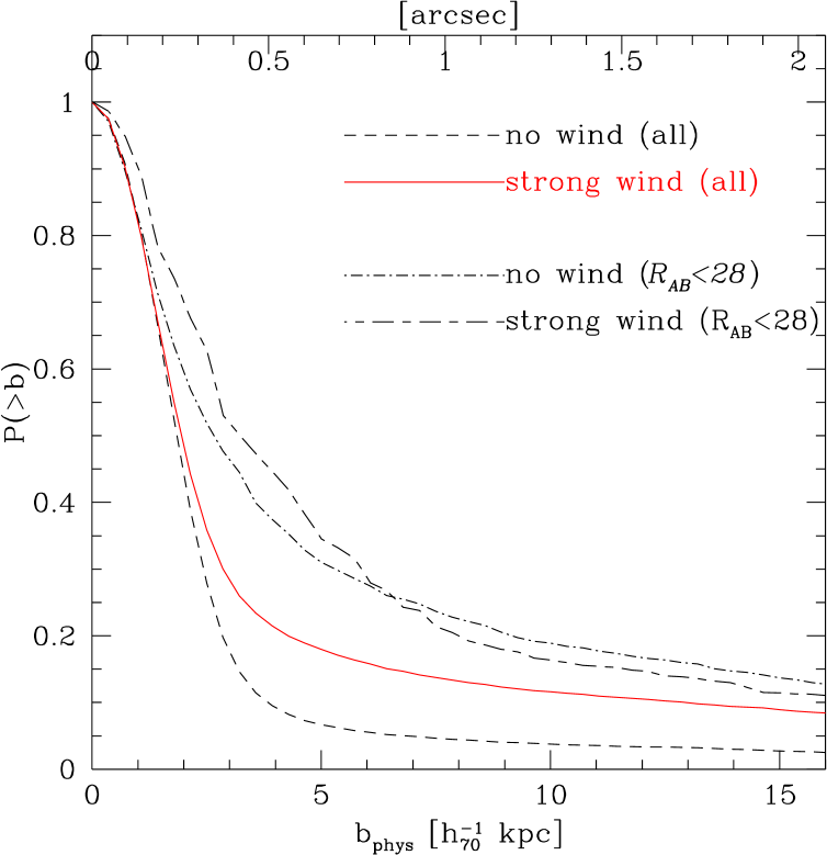
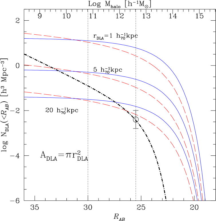
Figure 3: Left: Normalized impact parameter distribution for runs with and without galactic wind feedback. The results with limited search for the nearest galaxy to $R_{AB}<28$ mag are also shown. Right: Cumulative comoving number density of DLAs as a function of apparent $R_{AB}$ magnitude for three different values of assumed DLA physical radius $r_{\rm DLA}=1\,h_{70}^{-1}\,{\rm kpc}$, 5 $h_{70}^{-1}\,{\rm kpc}$, and 20 $h_{70}^{-1}\,{\rm kpc}$. The covering area of each DLA is $A_{\rm DLA}=\pi r_{\rm DLA}^{2}$. For each value of $r_{\rm DLA}$, results from no feedback run (long-dashed line) and strong feedback run (solid line) are shown. The thick dot-dashed line is the cumulative comoving number density of LBGs obtained by integrating the observed luminosity function[46]. The data point at $R_{AB}=25.5$ shows the observed comoving number density of LBGs $N_{\rm LBG}=4\times 10^{-3}h^{-3}\,{\rm Mpc}^{-3}$.

3.6 Number Density of DLAs

It would be useful to quantify the number density of DLAs similarly to the galaxy number density. However doing so is not easy both observationally and in numerical simulations, because DLA gas clouds are not detected in emission and they are often extended, connected, and exhibit very complicated morphologies as shown in Fig. 1 of Ref. NSH04b.

Theoretically, it is possible to calculate the mean number density of DLA clouds as follows. Assuming that the average physical covering area of each DLA gas cloud is fixed with $A_{\rm DLA}=\pi\,r_{\rm DLA}^{2}$, then the cumulative number density of DLAs above a certain halo mass $M$ is

$$N_{\rm DLA}(>M)=\int_{M}^{\infty}dM\,n_{\rm dm}(M)\,\frac{\sigma_{\rm DLA}^{\rm phys}(M)}{A_{\rm DLA}},$$ (6)

where $n_{\rm dm}(M)$ is the dark matter halo mass function, and $\sigma_{\rm DLA}^{\rm phys}(M)$ is the physical DLA cross section as a function of halo mass. Note that $\sigma_{\rm DLA}$ is the total DLA cross section of each dark matter halo; in other words, if there are 100 DLA clouds in a massive halo, then this halo has a total DLA cross section of $\sigma_{\rm DLA}^{\rm phys}=100\,A_{\rm DLA}$. Then, using Eq. (4) and (6), we calculate the cumulative comoving number density of DLAs as a function of apparent $R_{AB}$ magnitude $N_{\rm DLA}(<R_{AB})$ as shown in the right panel of Fig. 3. This figure shows that the number density of DLA clouds is higher than that of LBGs if their physical radius is smaller than $r_{\rm DLA}=20h_{70}^{-1}\,{\rm kpc}$. Based on a similar calculation, Ref. Schaye01a suggested possible relationship between outflows from LBGs and DLAs, although this idea is yet to be confirmed observationally.

3.7 Metallicity, $N_{\rm HI}$, and Star Formation Rate

Measurements of gas metallicity in DLAs and galaxies provide useful information on star formation and chemical enrichment history. The mean metallicity of DLAs is known[48] to be $\approx(1/30)Z_{\odot}$, and that of LBGs to be $\approx(1/3)Z_{\odot}$.

In Figure 4, we show the distribution of gas metallicity as functions of $N_{\rm HI}$ and projected star formation rate $\Sigma_{\rm SFR}$ for the two strong wind feedback runs (Q5 and G5 run) at $z=3$. The G5 run has a broader distribution than the Q5 run because of a larger box size (${\rm L_{box}}=100\,h^{-1}{\rm\,Mpc}$ for the G5 and $10\,h^{-1}{\rm\,Mpc}$ for the Q5 run), but lower median metallicity at lower $N_{\rm HI}$ values due to lower resolution. In the left panel, we see that there are no observed DLAs[49] with $\log N_{\rm HI}>22.0$ and $\log(Z/Z_{\odot})>-1.0$, while such sight-lines exist in our simulations. These columns with high $N_{\rm HI}$ and high metallicity are probably associated with central cores of LBGs that are actively forming stars. The occurrence of such columns are very rare as can be seen from the rapidly declining $f(N_{\rm HI})$ function, and they have very small cross-sections. There are other ideas to explain the absence of DLAs at $\log N_{\rm HI}>22.0$. One popular idea is the extinction of background quasars by dust[50, 51]. Another idea is that the conversion of H i to H₂ molecule determines the maximum value of $N_{\rm HI}$.[52] It is not fully clear at this point which of the above three explanations (or any combinations of them) is the correct one. At $\log N_{\rm HI}<22.0$, the Q5 run might be overpredicting the median metallicity of DLAs compared to observations.

The right panel of Fig. 4 shows a similar distribution as the left panel. This is because $\Sigma_{\rm SFR}$ and $N_{\rm HI}$ are correlated with each other strongly (i.e., $\Sigma_{\rm SFR}\propto N_{\rm HI}^{1.4}$, the Kennicutt Law[53]; see also Fig. 8 of Ref. NSH04b), and metallicity also correlates with star formation positively. The metallicity for the columns with $\log\Sigma_{\rm SFR}\gtrsim 0$ in the simulation might be slightly too high compared to the observational estimates of LBGs. The observational estimates by the C ii^∗ technique[54] (blue data points; only positive detections are shown) nicely fall onto the simulated contour.

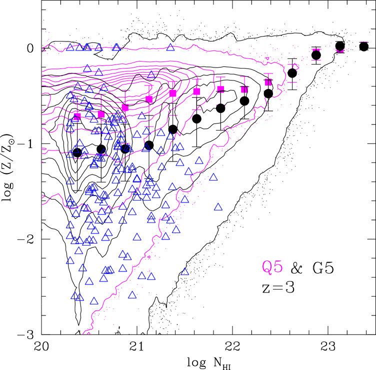
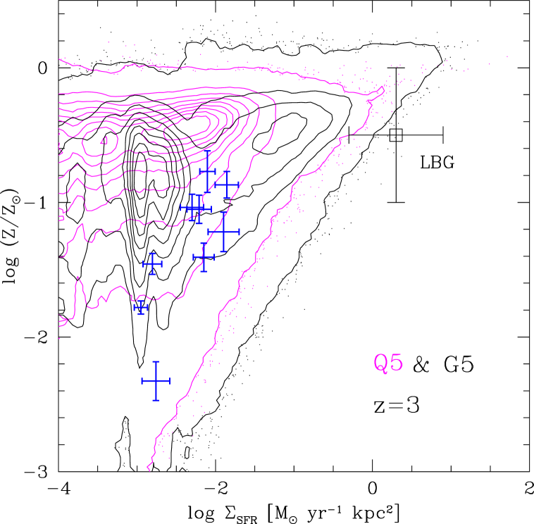
Figure 4: Left: Distribution of DLA columns on the plane of H i column density vs. metallicity are shown for the Q5 run (${\rm L_{box}}=10\,h^{-1}{\rm\,Mpc}$; magenta contour) and the G5 run (${\rm L_{box}}=100\,h^{-1}{\rm\,Mpc}$; black contour) at $z=3$ with the median points for each $\log N_{\rm HI}$ bin. The blue open triangles are observed data[49]. Right: Same as the left panel for the plane of projected star formation rate vs. metallicity. The skewed contour shape at $\log\Sigma_{\rm SFR}\approx-3$ for the G5 run is a resolution effect. The blue data points are observational estimates by the C ii^∗ technique[54], and the open square symbol represents LBGs roughly.

4 Predicting the [C II] Line Emission

The [C ii] emission line at $\lambda=157.74\,\mu$m originates from the ${}^{2}P_{3/2}\rightarrow^{2}P_{1/2}$ fine structure transition of C⁺. This emission line is often the brightest emission in the spectrum of galaxies, and it is suggested to be the dominant coolant of diffuse ISM at temperatures $T\leq 5000$ K.[55, 56, 57, 58] Therefore, it has been suggested that the [C ii] emission is potentially another method for finding cold neutral gas in high-$z$ universe.[59, 60]

Locally, [C ii] emission has been detected from both 1) dense star-forming gas irradiated by UV radiation from young stars[61, 62, 63, 64] and 2) extended, diffuse cold components of ISM in quiescent late-type galaxies[65, 66, 67, 68]. At high-$z$, there is only a few tentative detections[69, 70] of [C ii] emission from quasars at $z=6.42$ and $z=4.7$, but none for more normal (i.e., not quasars or active galactic nuclei) star-forming galaxies such as LBGs. Detections of [C ii] emission from LBGs, DRGs[71, 72], and star-forming BzK[73] galaxies might become possible in the near future by ALMA and SPICA.

We might be able to set important constraints on galaxy formation models using [C ii] detections. In particular interferometric maps of [C ii] emission would reveal the spatial dimensions of neutral gas that is responsible for DLAs, a property that has so far eluded detection. By combining these measurements with the velocity widths of the [C ii] emission lines, it will be possible to infer the dark matter halo masses of the sources, and the [C ii] luminosity would tell us the heating rate of the gas.

Ref. Nag06b attempted to make a realistic estimate of [C ii] emission from high-$z$ galaxies by coupling the analytic model of Ref. Wolfe03a and cosmological hydrodynamic simulations. We first used the star formation rate and metallicity of gas in our simulations to estimate the amount of cold neutral medium (CNM; typically $T\sim 100$ K and $n\sim 10$ cm^-3) in each halo, and then computed the [C ii] luminosity by multiplying the [C ii] luminosity per H i atom estimated by the analytic model to the CNM mass. As shown in the left panel of Fig. 5, we find that the [C ii] luminosity can be described roughly by

$$L_{\rm CII}=C_{1}\left(\frac{M_{\rm halo}}{10^{12}\,h^{-1}{\rm M_{\odot}}}\right),$$ (7)

where $C_{1}=10^{41}$  erg s^-1 (no wind) and $10^{40}$ erg s^-1 (strong wind feedback). The strong wind feedback reduces the amount of CNM by ejecting the gas from star-forming regions, resulting in lower [C ii] luminosity by a factor of $\sim 10$ compared to the no feedback run.

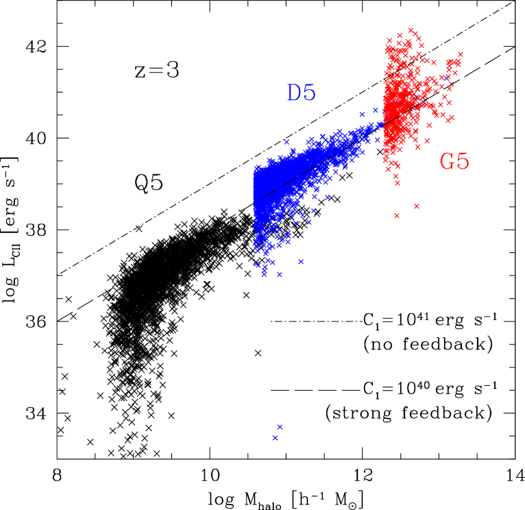
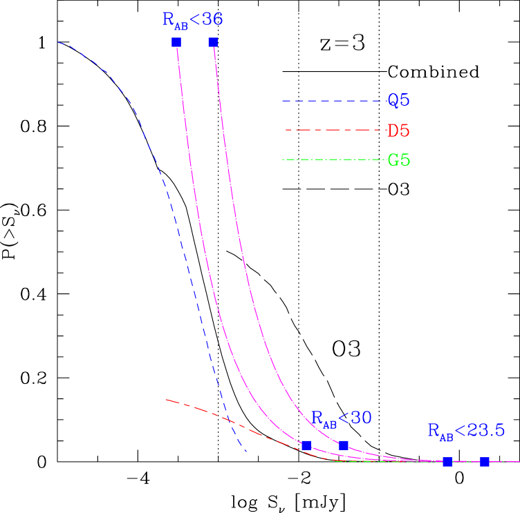
Figure 5: Left: [C ii] luminosity as a function of halo mass at $z=3$. The three sets of points are all from strong wind feedback runs: Q5, D5, and G6 runs with box sizes ${\rm L_{box}}=10,34$, and 100$h^{-1}{\rm\,Mpc}$, respectively. Right: Cumulative probability distribution function of [C ii] sources at $z=3$ as a function of flux density. The result from the run with no wind feedback (the O3 run with ${\rm L_{box}}=10h^{-1}{\rm\,Mpc}$, long-dashed line) is also shown. The two magenta dot-dashed lines are obtained[74] by integrating the observed luminosity function[46] of LBGs. The three vertical dotted lines indicate the flux density limits of $S_{\nu}=0.1,0.01,$ and 0.001 mJy. the diagram.

The right panel of Fig. 5 shows the probability distribution function of [C ii] sources at $z=3$ as a function of [C ii] flux density. For the runs with strong feedback, we see that only a few percent of all the sources would have [C ii] flux brighter than 1 mJy. Most of the [C ii] sources will be very faint, low-mass galaxies with $S_{\nu}<0.1$ mJy due to the large number of low-mass halos in a $\Lambda$CDM model. The run with no wind feedback gives more optimistic result in terms of the fraction of bright sources, suggesting that $\sim 30$% of [C ii] sources have $S_{\nu}>0.01$ mJy at $z=3$. These predictions can be tested by ALMA and SPICA in the future. Even though the [C ii] observation of normal high-$z$ galaxies is currently difficult, the reward of [C ii] detection from such sources would be quite significant, because such measurements could directly constrain the amount of CNM and the properties of ambient ISM, which is otherwise difficult to achieve.

The crude calculation by Ref. Nag06b was satisfactory as a first step, but we need to treat the radiation from local sources and the ionization of gas more accurately. To this end, we plan to use the photoionization code CLOUDY[76] and refine our [C ii] calculations in the future.

5 Conclusions & Future Research

In this article, we reviewed our DLA research using cosmological SPH simulations. We achieved some successes in explaining the global DLA statistics crudely, but there are details that need to be studied further. In particular, our simulations underpredict $f(N_{\rm HI})$ at $\log N_{\rm HI}<21.0$. To cure this problem, we need to make improvements on the following points: 1) increase mass and spatial resolution, 2) treat radiative transfer from local radiation sources and photoionization of gas more accurately, 3) improve the models for star formation and feedback. Also, our simulations are probably still suffering from the angular momentum transfer[77] problem, which we hope to remedy as we work on the above three points.

The possible connection between DLAs and LBGs is quite interesting. Ref. Wolfe03a detected the C ii^∗ $\lambda$1335.7 absorption in about a half of randomly selected DLAs, and showed that local heat sources (such as LBGs) are required to match the heating rate inferred from the [C ii] cooling rate. Their work and Ref. Cooke06a suggest close connection between DLAs and LBGs. It would be natural for the two population to be closely related to each other, considering the fact that DLAs are important reservoirs of neutral gas for star formation at high-$z$, and that LBGs contribute significantly to the total star formation rate density in high-$z$ universe.

Just like the multi-wavelength observations of galaxies can reveal different properties of galaxies, we can also tackle the mysteries of DLAs using different techniques including H i absorption, C ii^∗ and other metal line absorption, and [C ii] emission. Through continuous collaboration between observation and theory, we hope to clarify the physical nature of DLAs in the future.

References

- [1] J. P. Ostriker and P. J. Steinhardt, Nature 377, 600 (1995).
- [2] N. A. Bahcall, J. P. Ostriker, S. Perlmutter and P. Steinhardt, Science 284, 1481 (1999).
- [3] D. Spergel, L. Verde, H. V. Peiris, E. Komatsu, M. R. Nolta, C. L. Bennett, M. Halpern, G. Hinshaw et al., ApJS 148, 175 (2003).
- [4] A. M. Wolfe, D. A. Turnshek, H. E. Smith and R. D. Cohen, ApJS 61, 249 (1986).
- [5] A. M. Wolfe, E. Gawiser and J. X. Prochaska, ARA&A 43, 861 (2005).
- [6] K. M. Lanzetta, A. M. Wolfe and D. A. Turnshek, ApJ 440, 435 (1995).
- [7] L. J. Storrie-Lombardi and A. M. Wolfe, ApJ 543, 552 (2000).
- [8] C. Péroux, R. G. McMahon, L. J. Storrie-Lombardi and M. J. Irwin, MNRAS 346, 1103 (2003).
- [9] J. X. Prochaska, S. Herbert-Fort and A. M. Wolfe, ApJ 635, 123 (2005).
- [10] R. A. Jorgenson, A. M. Wolfe, J. X. Prochaska, L. Lu, J. C. Howk, J. Cooke, E. Gawiser and D. M. Gelino, ApJ 646, 730 (2006).
- [11] P. Madau, H. C. Ferguson, E. D. Dickinson, M. Giavalisco, C. C. Steidel and A. Fruchter, MNRAS 283, 1388 (1996).
- [12] C. C. Steidel, K. L. Adelberger, M. Giavalisco, M. Dickinson and M. Pettini, ApJ 519, 1 (1999).
- [13] K. Nagamine, M. Fukugita, R. Cen and J. P. Ostriker, ApJ 558, 497 (2001).
- [14] L. Hernquist and V. Springel, MNRAS 341, 1253 (2003).
- [15] M. Ouchi, K. Shimasaku, H. Furusawa, M. Miyazaki, M. Doi, M. Hamabe, T. Hayashino, M. Kimura et al., ApJ 611, 660 (2004a).
- [16] A. M. Hopkins and J. F. Beacom, ApJ 651, 142 (2006).
- [17] D. G. York et al., AJ 120, 1579 (2000).
- [18] J. X. Prochaska and A. M. Wolfe, ApJ 487, 73 (1997).
- [19] M. Haehnelt, M. Steinmetz and M. Rauch, ApJ 495, 647 (1998).
- [20] A. H. Maller, J. X. Prochaska, R. S. Somerville and J. R. Primack, MNRAS 326, 1475 (2001).
- [21] G. Kauffmann, MNRAS 281, 475 (1996).
- [22] K. Okoshi, M. Nagashima, N. Gouda and S. Yoshioka, ApJ 603, 12 (2004).
- [23] K. Nagamine, V. Springel and L. Hernquist, MNRAS 348, 421 (2004).
- [24] K. Nagamine, V. Springel and L. Hernquist, MNRAS 348, 435 (2004).
- [25] J. Gardner, N. Katz, L. Hernquist and D. H. Weinberg, ApJ 484, 31 (1997a).
- [26] J. Gardner, N. Katz, D. H. Weinberg and L. Hernquist, ApJ 486, 42 (1997b).
- [27] J. Gardner, N. Katz, L. Hernquist and D. H. Weinberg, ApJ 559, 131 (2001).
- [28] A. O. Razoumov, M. L. Norman, J. X. Prochaska and A. M. Wolfe, ApJ 645, 55 (2006a).
- [29] V. Springel and L. Hernquist, MNRAS 333, 649 (2002).
- [30] F. Haardt and P. Madau, ApJ 461, 20 (1996).
- [31] N. Katz, D. H. Weinberg and L. Hernquist, ApJS 105, 19 (1996).
- [32] R. Davé, L. Hernquist, N. Katz and D. H. Weinberg, ApJ 511, 521 (1999).
- [33] V. Springel and L. Hernquist, MNRAS 339, 312 (2003).
- [34] V. Springel and L. Hernquist, MNRAS 339, 289 (2003).
- [35] M. A. Zwaan and J. X. Prochaska, ApJ 643, 675 (2006).
- [36] W. H. Press and P. Schechter, ApJ 187, 425 (1974).
- [37] R. K. Sheth and G. Tormen, MNRAS 308, 119 (1999).
- [38] K. Nagamine, A. M. Wolfe, L. Hernquist and V. Springel, ApJ 660, 945 (2007).
- [39] J. Cooke, A. M. Wolfe, E. Gawiser and J. X. Prochaska, ApJL 636, L9 (2006).
- [40] J. Cooke, A. M. Wolfe, E. Gawiser and J. X. Prochaska, ApJ 652, 994 (2006).
- [41] N. Bouche, J. P. Gardner, D. H. Weinberg, R. Davé and J. D. Lowenthal, ApJ 628, 89 (2005).
- [42] D. R. Law, C. C. Steidel, D. K. Erb, M. Pettini, N. A. Reddy, A. E. Shapley, K. L. Adelberger and D. J. Simenc, ApJ 656, 1 (2007).
- [43] P. Møller, J. U. Fynbo and S. M. Fall, A&A 422, L33 (2004).
- [44] H.-W. Chen, J. X. Prochaska, B. J. Weiner, J. S. Mulchaey and G. M. Williger, ApJL 629, L25 (2005).
- [45] E. Gawiser, A. M. Wolfe, J. X. Prochaska, K. M. Lanzetta, N. Yahata and A. Quirrenbach, ApJ 562, 628 (2001).
- [46] K. L. Adelberger and C. C. Steidel, ApJ 544, 218 (2000).
- [47] J. Schaye, ApJ 559, L1 (2001).
- [48] M. Pettini, Element abundances through the cosmic ages, in Cosmochemistry. The melting pot of the elements, eds. C. Esteban, R. García López, A. Herrero and F. a.-p. Sánchez2004.
- [49] J. X. Prochaska, A. M. Wolfe, J. C. Howk, E. Gawiser, S. M. Burles and J. Cooke, ApJS 171, 29 (2007).
- [50] S. M. Fall and Y. C. Pei, ApJ 402, 479 (1993).
- [51] G. Vladilo and C. Péroux, A&A 444, 461 (2005).
- [52] J. Schaye, ApJ 562, L95 (2001).
- [53] R. C. J. Kennicutt, ApJ 498, 541 (1998).
- [54] A. M. Wolfe, E. Gawiser and J. X. Prochaska, ApJ 593, 235 (2003).
- [55] A. Dalgarno and R. A. McCray, ARA&A 10, 375 (1972).
- [56] A. G. G. M. Tielens and D. Hollenbach, ApJ 291, 722 (1985).
- [57] M. G. Wolfire, D. Hollenbach, C. F. McKee, A. G. G. M. Tielens and E. L. O. Bakes, ApJ 443, 152 (1995).
- [58] N. Lehner, B. P. Wakker and B. D. Savage, ApJ 615, 767 (2004).
- [59] V. Petrosian, J. N. Bahcall and E. E. Salpeter, ApJL 155, L57 (1969).
- [60] A. Loeb, ApJL 404, L37 (1993).
- [61] R. W. Russell, G. Melnick, G. E. Gull and M. Harwit, ApJL 240, L99 (1980).
- [62] M. K. Crawford, R. Genzel, C. H. Townes and D. M. Watson, ApJ 291, 755 (1985).
- [63] G. J. Stacey, N. Geis, R. G. ad J. B. Lugten, A. Poglitsch, A. Sternberg and C. H. Townes, ApJ 373, 423 (1991).
- [64] P. Carral, D. J. Hollenbach, S. D. Lord, S. W. J. Colgan, M. R. Haas, R. H. Rubin and E. F. Erickson, ApJ 423, 223 (1994).
- [65] S. C. Madden, N. Geis, R. Genzel, F. Herrmann, J. Jackson, A. Poglitsch, G. J. Stacey and C. H. Townes, ApJ 407, 579 (1993).
- [66] K. J. Leech, H. J. Völk, I. Heinrichsen, H. Hippelein, L. Metcalfe, D. Pierini, C. C. Popescu, R. J. Tuffs and C. Xu, MNRAS 310, 317 (1999).
- [67] S. Malhotra, M. J. Kaufman, D. Hollenbach, G. Helou, R. H. Rubin, J. Brauher, D. Dale, N. Y. Lu et al., ApJ 561, 766 (2001).
- [68] A. Contursi, M. J. Kaufman, G. Helou, D. J. Hollenbach et al., AJ 124, 751 (2002).
- [69] R. Maiolino, P. Cox, P. Caselli, A. Beelen, F. Bertoldi, C. L. Carilli, M. J. Kaufman, K. M. Menten et al., A&A 440, L51 (2005).
- [70] D. Iono, M. S. Yun, M. Elvis, A. B. Peck, P. T. P. Ho, D. J. Wilner, T. R. Hunter, S. Matsushita and S. Muller, ApJ 645, L97 (2006).
- [71] M. Franx, I. Labbe, G. Rudnick, P. G. van Dokkum, E. Daddi, S. Förster, M. Natascha, A. Moorwood et al., ApJ 587, L79 (2003).
- [72] P. van Dokkum, M. Franx, N. F. Schreiber, G. Illingworth, E. Daddi, K. K. Knudsen, I. Labbe, A. Moorwood et al., ApJ 611, 703 (2004).
- [73] E. Daddi, A. Cimatti, A. Renzini, A. Fontana, M. Mignoli, L. Pozzetti, P. Tozzi and G. Zamorani, ApJ 617, 746 (2004).
- [74] K. Nagamine, A. M. Wolfe and L. Hernquist, ApJ 647, 60 (2006).
- [75] A. M. Wolfe, J. X. Prochaska and E. Gawiser, ApJ 593, 215 (2003).
- [76] G. J. Ferland, K. T. Korista, D. A. Verner, J. W. Ferguson, J. B. Kingdon and E. M. Verner, PASP 110, 761 (1998).
- [77] T. Kaufmann, L. Mayer, J. Wadsley, J. Stadel and B. Moore, MNRAS 375, 53 (2007).