One-Electron Physics of the Actinides

Abstract

We present a detailed analysis of the one-electron physics of the actinides. Various LMTO basis sets are analyzed in order to determine a robust bare Hamiltonian for the actinides. The hybridization between $f$- an $spd$- states is compared with the $f-f$ hopping in order to understand the Anderson-like and Hubbard-like contributions to itineracy in the actinides. We show that both contributions decrease strongly as one move from the light actinides to the heavy actinides, while the Anderson-like contribution dominates in all cases. A real-space analysis of the band structure shows that nearest-neighbor hopping dominates the physics in these materials. Finally, we discuss the implications of our results to the delocalization transition as function of atomic number across the actinide series.

I Introduction

I.1 Background of the actinides

It is well acceptedPu_Futures that the actinides are divided into two groups based on the behavior of the $f$-electrons. The lighter actinides (Th to Pu) have smaller atomic volumes, low-symmetry crystal structures and itinerant $5f$ states that participate in metallic bondingSoderlind95 . Alternatively, the heavy actinides (Am to Es) have larger atomic volumes, high-symmetry crystal structures, and relatively localized $f$-electrons. Applying pressure to the heavy actinides results in a series of crystallographic phase transitions, and the respective phases often have significantly different volumes Heathman2005 ; Lindbaum2001 . Transitions of this sort are often referred to as ”volume collapse” transitions. Given that the application of ample pressure to any system of localized electrons will eventually cause a delocalization transition, understanding what role the electronic delocalization transition may play in the volume collapse transition has been and continues to be an active area of study Savrasov2001 ; Soderlind2004 .

Plutonium is considered to be the dividing line of actinide series, with the $\alpha$- and $\delta$- phases associated with light and heavy behavior, respectively. This dual nature of Pu, along with an enormous $25\%$ volume collapse for the $\delta\rightarrow\alpha$ transition, has made Pu the most interesting element among the $5f$ compounds for basic theoretical research over the past 50 years Freeman84 ; Lashley2005 .

The actinides are among the most complicated classes of materials in terms of understanding electronic correlations given the presence of $s$, $p$, $d$, and $f$ electrons near the Fermi surface and the unusual behavior observed in experiment. Broad discussion in the literature was devoted to the following topics: abrupt change in volume and bulk modulusSkriver78 ; unique crystal structuresSoderlind95 ; partial localization of $f$-electronsEriksson99 , Mott transition Johansson74 ; Johansson75 ; paramagnetism in light actinides and formation of magnetic moments in heavier actinides (starting from Cm)Lashley2005 . For this purpose numerous Ab Initio electronic structure calculations have been performed for the actinides. The techniques such as LDA Ek93 ; Jones2000 , GGASoderlind97 , SIC-LSDSvane2007 , LDA+U Savrasov2000 ; Shorikov05 ; Shick2005 and DMFT-based approaches Zhu2007 ; Shim2006 ; Pourovskii2007 have been implementedAnisimov2006 .

I.2 Actinide Hamiltonian

The model Hamiltonian for the actinides can be written as:

$$H=\sum_{ija\beta}V_{ija\beta}(c^{\dagger}_{ai}f_{\beta j}+c.c.)+\sum_{ij\alpha\beta}t^{f}_{ij\alpha\beta}f^{\dagger}_{\alpha i}f_{\beta j}$$ (1)

$$+\sum_{\mathbf{k}ab}t^{spd}_{ab}(\mathbf{k})c^{\dagger}_{\mathbf{k}a}c_{\mathbf{k}b}+\sum_{i\alpha\beta\gamma\delta}U_{\alpha\beta\gamma\delta}f^{\dagger}_{\alpha i}f^{\dagger}_{\beta i}f_{\gamma i}f_{\delta i}$$

where $f_{\alpha i}$ is the annihilation operator for $5f$-electron in state $\alpha=|j,j_{z}\rangle$ at site $i$, and $c_{ai}$ is annihilation operator for conduction electrons in the state $a=|n,j^{\prime},j^{\prime}_{s}\rangle$. This model can be understood as a periodic Anderson model in which additional direct hopping is allowed between the correlated states. Equivalently, this model can be thought of as a Hubbard model with additional uncorrelated states that hybridize with the correlated states. Therefore, the model for the actinides contains the physics of both the periodic Anderson model and the Hubbard model. In the Hubbard model $t^{f}$ competes with $U$ to determine the degree of localization of the electrons, while in the periodic Anderson model $V$ competes with $U$. In the model of the actinides $t^{f}$ and $V$ cooperatively compete with $U$, and the relative magnitudes of $t^{f}$ and $V$ will determine the degree of Hubbard-like and Anderson-like contributions to the itineracy of the $f$-electrons. The main focus of this study is to determine the relative importance of $t^{f}$ and $V$ across the actinide series. This is a first step towards a detailed understanding of the quantitative aspects of the localization-delocalization transition in the actinide series.

Hamiltonians of the form described in Eq. (1) containing heavy and light electrons have appeared in various contexts in condensed matter physics. To deal with this complexity, this model is often reduced to a simpler model by eliminating the light electrons (i.e. $spd$ states) to obtain an effective Hubbard model having only the heavy (i.e. $f$) states. The reduced model only describes the bands within a narrow energy window around the Fermi energy (i.e. $\sim$1eV). The new renormalized $f$ hoppings have contributions from both the original $f$ hopping in addition to the $spd$ hopping. Additionally, many new interactions terms are generated, but these are usually ignored and only the on-site coulomb repulsion is retained as in the original hamiltonian. This procedure of one-electron ”downfolding” has been used extensively to study electronic correlations in the transition-metal oxides, and there has been success in describing the photoemission spectra in this manner. In the context of the actinides, it is not clear that this approach is justified. Perhaps the most important issue is the nature of the localization transition in the actinide series. In the Hubbard model, when $U$ is sufficiently large the effective $f$ states will be localized and the system will be insulating. In the actinide model, when $U$ is sufficiently large the $f$ states will be localized, but the system will not necessarily be an insulator. It is possible that the $spd$ states may still form a Fermi surface and give rise to a metallic state. Therefore, the actinide model and the effective Hubbard model differ even at a qualitative level in certain regimes. Some aspects of localization-delocalization in the actinide model and the Hubbard model treated by DMFT are very similar at intermediate temperatures Held2000 (for example they both exhibit a line of first order phase transitions ending at a second order point), but there are significant differences at very low temperatures when hybridization becomes a relevant perturbation suppressing Mott transition Medici2005 . Furthermore, the behavior at large $U$ and high temperatures should be quite different in the two models, due to the presence of the broad metallic $spd$ bands in the actinide model. Due to these considerations, we pursue the actinide model which should be a more accurate representations of the actinides given that the Hubbard model is an approximate reduction of the actinide model.

In general, the parameters $V$ and $t^{f}$ depend on the choice of basis set and therefore are not unique. This, of course, does not affect the band structure which is basis independent, but becomes an important in the context of approximate many body treatments (such as DMFT) which include only local Coulomb on the $f$ orbitals. For this purposes it is clearly advantageous to set up a Hamiltonian in an orthogonal basis where the $f$ electrons are highly localized. Hence, the secondary objective of this work is to determine a good basis set for setting up models of the actinides. For earlier tight-binding parametrization for actinides see Ref. Harrison83 ; Harrison87 ; Zhu2007 .

I.3 Motivation for this work

The idea of a localization-delocalization transition in the actinides was brought forward by JohanssonJohansson74 . Johansson based this idea on an empirical comparison of the canonical $5f$-bandwidth with the estimates of the Coulomb interaction in the form of a Hubbard $U$, and therefore he is starting with the assumption of a Hubbard model to represent the actinides. As a result, the localization-delocalization transition is designated as a Mott transition in his paper, but it should be realized that this is a consequence of starting with an assumption of a Hubbard model. For a later elaboration of these ideas in the context of the $\alpha$-$\delta$ transition in Pu see Ref.Katsnelson92 ; Severin92 .

The important role of $d-f$ hybridization in actinide metals and alloys was stressed in the early work of Jullien et al.Jullien72 ; Jullien73 who considered models similar to Eq. (1).

In this paper, we reconsider the issue of the description of the localization-delocalization transition in the actinide series from a perspective which is motivated by recent DMFT and LDA+DMFT worksShim2006 ; Pourovskii2007 ; Zhu2007 . These works utilize the actinide hamiltonian (i.e. both $f$ and $spd$ states are included), and have provided further demonstration of the hypothesis that a localization-delocalization transition takes place across the actinide series. However, the relative importance of $t^{f}$ and $V$ (i.e. Hubbard-like vs. Anderson-like contributions) were not explicitly examined in these studies.

II Orbitals and Basis

II.1 Basis set dependence issue

While the issue of representing the Kohn-Sham hamiltonian in different basis sets has been a subject of numerous studies, the dependence of the results of correlated electronic structure methods such as LDA+DMFT on the choice of correlated orbitals is only beginning to be exploredsolovyev .

In this study, we investigate the role of the choice of the correlated $f$ orbital. We first take the $f$ electron orbital as the $f$ element of the LMTO basis, both in the bare and screened representationsSkriver84 ; Andersen84 . The LMTO basis is non-orthogonal and therefore must be orthogonalized in order to avoid the complications of solving the many-body problem in a non-orthogonal basis. As we will show in this study, the method of orthogonalization has a large influence on the results. We utilize both the Löwdin orthogonalizationLowdin50 and the projective orthogonalizationKristjan2006 ; Shim2006 that was used in earlier implementations of LDA+DMFT. This effectively results in four different constructions of $f$ orbitals, listed in Table 1.

Table 1: Choice of basis.

Bare LMTO	Screened LMTO
Löwdin transform	Löwdin transform
Bare LMTO	Screened LMTO
projective basis	projective basis

II.2 Bare and Screened LMTO within ASA scheme

The basis set of linear muffin-tin orbitals (LMTOs) has been extensively used in electronic structure calculations Skriver84 ; Turek96 . Within the atomic sphere approximation (ASA), LMTO is a minimal and efficient basis set with one basis function per site $I$ and quantum pair $L=(l,m)$. Although the LMTO method is physically transparent, the constructed basis is non-orthogonal.

Below we sketch the derivation of the bare and screened LMTO basis set within the ASA. The construction of the bare LMTOs $\chi_{IL}(\mathbf{r})$ starts with so called envelope function Turek96 , which is a decaying solution of the Laplace equation centered at the site $I$:

$$K_{L}(\mathbf{r}_{I})=K_{l}(r_{I})Y_{L}(\hat{\mathbf{r}}_{I})=\left(\frac{w}{r_{I}}\right)^{l+1}Y_{L}(\hat{\mathbf{r}}_{I}),$$ (2)

here $\mathbf{r}_{I}=\mathbf{r}-\mathbf{R}_{I}$, unit vector $\hat{\mathbf{r}}_{I}$ indicates the direction of $\mathbf{r}_{I}$, $Y_{L}(\hat{\mathbf{r}}_{I})$ is a spherical function, and $w$ is a scaling parameter associated with the linear size of unit cell.

In any atomic sphere other than $I$, $K_{L}(\mathbf{r}_{I})$ can be represented as:

$$K_{L}(\mathbf{r}_{I})=-\sum_{L^{\prime}}S_{IL,I^{\prime}L^{\prime}}J_{L^{\prime}}(\mathbf{r}_{I^{\prime}}).$$ (3)

The function $J_{L}(\mathbf{r}_{I})=(r_{I}/w)^{l}Y_{L}(\hat{\mathbf{r}}_{I})$ stands for the regular solutions of Laplace equation, and $S_{IL,I^{\prime}L^{\prime}}$ are structure constants.

Inside each atomic sphere we construct a linear combination of the solution $\phi_{IL}(\mathbf{r}_{I})$ of the Schrödinger equation and its first derivative with respect to energy $\dot{\phi}_{IL}(\mathbf{r}_{I})$ at some fixed energy $E_{\nu}$.

The final step is to smoothly match the boundary conditions at the surface of sphere $I$:

$$\Phi^{H}_{L}(\mathbf{r}_{I})\equiv A^{K}_{IL}\phi_{IL}(\mathbf{r}_{I})+B^{K}_{IL}\dot{\phi}_{IL}(\mathbf{r}_{I})\rightarrow K_{L}(\mathbf{r}_{I})$$ (4)

and at the surface of sphere $I^{\prime}$ for all $I^{\prime}\neq I$:

$$\Phi^{J}_{L^{\prime}}(\mathbf{r}_{I^{\prime}})\equiv A^{J}_{I^{\prime}L^{\prime}}\phi_{I^{\prime}L^{\prime}}(\mathbf{r}_{I^{\prime}})+B^{J}_{I^{\prime}L^{\prime}}\dot{\phi}_{I^{\prime}L^{\prime}}(\mathbf{r}_{I^{\prime}})\rightarrow J_{L^{\prime}}(\mathbf{r}_{I^{\prime}}).$$ (5)

With the array of constants A and B determined from (4) - (5) we conclude the construction of bare LMTO basis function:

$$\chi_{IL}(\mathbf{r}_{I})=\left\{\begin{array}[]{ll}\Phi^{H}_{L}(\mathbf{r}_{I}),&\mathbf{r}_{I}\in S_{I},\\ -\sum_{I^{\prime}L^{\prime}}S_{IL,I^{\prime}L^{\prime}}\Phi^{J}_{L^{\prime}}(\mathbf{r}_{I^{\prime}}),&\mathbf{r}_{I^{\prime}}\in S_{I^{\prime}}(I\neq I^{\prime}),\\ K_{L}(\mathbf{r}_{I}),&\mathbf{r}\in Interstitial.\end{array}\right.$$ (9)

The Fourier transform of the LMTOs with respect to $\mathbf{R}_{I}-\mathbf{R}_{I^{\prime}}$ gives:

$$\chi_{\mathbf{k}L}(\mathbf{r})=\left\{\begin{array}[]{ll}\Phi^{H}_{L}(\mathbf{r})-\sum_{L^{\prime}}\Phi^{J}_{L^{\prime}}(\mathbf{r})S_{\mathbf{k}LL^{\prime}},&|\mathbf{r}|\leq R_{MT},\\ \sum_{\mathbf{k}}e^{i\mathbf{k}\mathbf{R}}K_{L}(\mathbf{r}-\mathbf{R}),&|\mathbf{r}|>R_{MT}.\\ \end{array}\right.$$ (12)

The standard LMTO method outlined above yields long-range orbitals. The concept of a screened LMTO was created to overcome the non-locality of the bare LMTO basis set Andersen84 . The method is based upon the idea of localizing the LMTOs by screening with multipoles added on the neighboring spheres. Namely, to each regular solution of Laplace equation we add $-\alpha_{IL}$ of the irregular solution:

$$J^{\alpha}_{L}(\mathbf{r}_{I})=J_{L}(\mathbf{r}_{I})-\alpha_{IL}K_{L}(\mathbf{r}_{I}).$$ (13)

The condition that on-site Laplace solution should not change leads to the Dyson-like equation for the screened structure constants:

$$S^{\alpha}_{a,a^{\prime}}=S_{a,a^{\prime\prime}}[\delta_{a^{\prime\prime}a^{\prime}}+\alpha_{a^{\prime\prime}}S^{\alpha}_{a^{\prime\prime},a^{\prime}}]=S_{a,a^{\prime\prime}}U_{a^{\prime\prime},a^{\prime}},$$ (14)

where matrix index $a$ refers to the pair $(I,L)$ and implies summation over repeated indices. The matrices $\alpha_{a}\equiv\alpha_{l}$ are diagonal for each $l$. In our calculations the choice of $\alpha$’s was as follows: $\alpha_{s}=5.5166$, $\alpha_{p}=0.5242$, $\alpha_{d}=0.1382$ and $\alpha_{f}=0.0355.$

The screened and bare envelope functions are related by the transformation $U_{a^{\prime},a}$ introduced in (14):

$$K^{\alpha}_{L}(\mathbf{r}_{I})=\sum_{I^{\prime}L^{\prime}}K_{L^{\prime}}(\mathbf{r}_{I^{\prime}})[\delta_{I^{\prime}L^{\prime},IL}+\alpha_{I^{\prime}L^{\prime}}S^{\alpha}_{I^{\prime}L^{\prime}IL}],$$ (15)

Or in matrix notations:

$$K^{\alpha}_{a}=K_{a^{\prime}}U_{a^{\prime},a},$$

where $K_{a}\equiv K_{L}(\mathbf{r}_{I})$ and $K^{\alpha}_{a}\equiv K^{\alpha}_{L}(\mathbf{r}_{I}).$

With the definitions (13), (14) and (15) the construction of screened LMTOs proceeds exactly in the same way as in the case of the bare LMTOs. Namely, we construct new linear combinations

$$\Phi^{H\alpha}_{L}(\mathbf{r}_{I})\equiv A^{K\alpha}_{IL}\phi_{IL}(\mathbf{r}_{I})+B^{K\alpha}_{IL}\dot{\phi}_{IL}(\mathbf{r}_{I})$$

inside the sphere $I$ by matching smoothly $K^{\alpha}_{L}(\mathbf{r}_{I})$ on its surface. Also, we construct new linear combination

$$\Phi^{J\alpha}_{L^{\prime}}(\mathbf{r}_{I^{\prime}})\equiv A^{J\alpha}_{I^{\prime}L^{\prime}}\phi_{I^{\prime}L^{\prime}}(\mathbf{r}_{I^{\prime}})+B^{J\alpha}_{I^{\prime}L^{\prime}}\dot{\phi}_{I^{\prime}L^{\prime}}(\mathbf{r}_{I^{\prime}})$$

inside sphere $I^{\prime}$ by matching smoothly $J^{\alpha}_{L^{\prime}}(\mathbf{r}_{I^{\prime}})$ on its surface for each $I^{\prime}\neq I$. Thus, we arrive to the definition of the screened LMTO:

$$\chi^{\alpha}_{IL}(\mathbf{r}_{I})=\left\{\begin{array}[]{ll}\Phi^{H\alpha}_{L}(\mathbf{r}_{I}),&\mathbf{r}_{I}\in S_{I},\\ -\sum_{I^{\prime}L^{\prime}}S^{\alpha}_{IL,I^{\prime}L^{\prime}}\Phi^{J\alpha}_{L^{\prime}}(\mathbf{r}_{I^{\prime}}),&\mathbf{r}_{I^{\prime}}\in S_{I^{\prime}}(I\neq I^{\prime}),\\ K^{\alpha}_{L}(\mathbf{r}_{I}),&\mathbf{r}\in Interstitial.\end{array}\right.$$ (19)

The Fourier transform of the screened LMTOs with respect to $\mathbf{R}_{I}-\mathbf{R}_{I^{\prime}}$ gives:

$$\chi^{\alpha}_{\mathbf{k}L}(\mathbf{r})=\left\{\begin{array}[]{ll}\Phi^{H\alpha}_{L}(\mathbf{r})-\sum_{L^{\prime}}\Phi^{J\alpha}_{L^{\prime}}(\mathbf{r})S_{\mathbf{k}LL^{\prime}},&|\mathbf{r}|\leq R_{MT},\\ \sum_{\mathbf{k}}e^{i\mathbf{k}\mathbf{R}}K^{\alpha}_{L}(\mathbf{r}-\mathbf{R}),&|\mathbf{r}|>R_{MT}.\\ \end{array}\right.$$ (22)

The Hamiltonian and overlap matrices in screened and bare LMTO representations ($O$ , $H$, and $O^{\alpha}$, $H^{\alpha}$ respectively) are related through the transformation $U$ introduced in (14):

$$H^{\alpha}=U^{\dagger}HU$$ (23)

$$O^{\alpha}=U^{\dagger}OU.$$ (24)

Having constructed the basis, one has to solve the generalized eigenvalue problem:

$$(H(\mathbf{k})-\epsilon_{i}(\mathbf{k})O(\mathbf{k}))\psi_{i}(\mathbf{k})=0.$$ (25)

As described above, it is necessary to transform to an orthogonal basis when performing many-body calculations, such as DMFT, in order to avoid the difficulties associated with a non-orthogonal basis.

II.3 Löwdin orthogonalization

Löwdin orthogonalization Lowdin50 is a straightforward orthogonalization of the Hamiltonian which uses no information from the basis set:

$$\tilde{\mathcal{H}}(\mathbf{k})=\frac{1}{\sqrt{O^{\dagger}(\mathbf{k})}}\mathcal{H}(\mathbf{k})\frac{1}{\sqrt{O(\mathbf{k})}}.$$ (26)

As will be shown below, this orthogonalization procedure may lead to a further mixing of $L$ characters among the LMTOs and hence unphysical results.

II.4 Projective orthogonalization

A physically motivated orthogonalization procedure is to find a basis where each function contains the maximum amount of a particular $L$ character. This approach proposed by K. Haule was used in earlier LDA+DMFT studies of Cerium and Plutonium Kristjan2006 . This basis has an important advantage, being that the ”$f$ electron” in this basis has maximal $f$ character. Mathematically, the non-interacting spectral function of the $f$ electron Green’s function in this basis agrees with the LDA projected density-of-states having $f$ character, as shown in Appendix A. This allowed us to identify the $f$ occupation in this basis set with the occupation numbers inferred from EELS and X-Ray absorption which are sensitive to angular momentum selection rulesmoore .

Here we follow Ref.Kristjan2006 . It is straightforward using (12) and (24) to show that overlapping matrix within MT-sphere can be represented as Andersen85 :

$$O_{\mathbf{k}L_{1}L_{2}}=\delta_{L_{1}L_{2}}o^{(HH)}_{l_{1}}-S^{\dagger}_{\mathbf{k}L_{1}L_{2}}o^{(JH)}_{l_{2}}-o^{(HJ)}_{l_{1}}S_{\mathbf{k}L_{1}L_{2}}$$ (27)

$$+S^{\dagger}_{\mathbf{k}L_{1}L^{\prime}}o^{(JJ)}_{l^{\prime}}S_{\mathbf{k}L^{\prime}L_{2}}.$$

The quantities $o^{HH}_{l}$, $o^{JH}_{l}$, $o^{HJ}_{l}$ and $o^{JJ}_{l}$ are numbers in each $l$-subspace. For $A$ and $B$ representing $H$ or $J$:

$$o^{AB}_{l_{1}}=\langle\Phi^{A}_{L_{1}}|\Phi^{B}_{L_{2}}\rangle\delta_{L_{1}L_{2}},$$ (28)

In each $L$-subspace the overlapping matrix is:

$$O_{\mathbf{k}}=o^{(HH)}-S^{\dagger}_{\mathbf{k}}o^{(JH)}-o^{(HJ)}S_{\mathbf{k}}+S^{\dagger}_{\mathbf{k}}o^{(JJ)}S_{\mathbf{k}}.$$ (29)

In order to find the transformation to the orthonormal base we must represent $O(\mathbf{k})$ as the square of a matrix. As we show below, the most intelligent choice would be:

$$O(\mathbf{k})\approx(\mathcal{H}-\mathcal{J}S_{\mathbf{k}})^{\dagger}(\mathcal{H}-\mathcal{J}S_{\mathbf{k}})$$ (30)

for each $L$-subspace. Here $\mathcal{H}$ and $\mathcal{J}$ are diagonal matrices proportional to unity in each subspace of definite $L$ just like the overlaps $o^{(HH)}$ defined above.

The above equation can not be made exact because the overlap numbers are obtained by integration over the radial part of wave functions. However, in most cases the overlap numbers can become very close to their approximations:

$$\begin{array}[]{ccc}o^{(HH)}_{l}&\approx&\mathcal{H}^{*}_{l}\mathcal{H}_{l},\\ o^{(JH)}_{l}&\approx&\mathcal{J}^{*}_{l}\mathcal{H}_{l},\\ o^{(HJ)}_{l}&\approx&\mathcal{H}^{*}_{l}\mathcal{J}_{l},\\ o^{(JJ)}_{l}&\approx&\mathcal{J}^{*}_{l}\mathcal{J}_{l}.\\ \end{array}$$ (31)

For each $L$ we have three independent equations for two unknowns. An approximate solution can be found by minimizing the following function:

$$|o^{(HH)}_{l}-\mathcal{H}^{*}_{l}\mathcal{H}_{l}|^{2}+|o^{(JH)}_{l}-\mathcal{J}^{*}_{l}\mathcal{H}_{l}|^{2}$$ (32)

$$+|o^{(HJ)}_{l}-\mathcal{H}^{*}_{l}\mathcal{J}_{l}|^{2}+|o^{(JJ)}_{l}-\mathcal{J}^{*}_{l}\mathcal{J}_{l}|^{2}=min.$$

The desired transformation to the new base is:

$$T_{\mathbf{k}}=(\mathcal{H}-\mathcal{J}S_{\mathbf{k}})^{-1}.$$ (33)

Finally:

$$\begin{array}[]{cccc}O_{\mathbf{k}}^{new}&=&T^{\dagger}_{\mathbf{k}}O_{\mathbf{k}}T_{\mathbf{k}}&\approx 1,\\ H_{\mathbf{k}}^{new}&=&T^{\dagger}_{\mathbf{k}}H_{\mathbf{k}}T_{\mathbf{k}}.\\ \end{array}$$ (34)

III Results

We perform relativistic, spin-restricted LDA calculations within the ASA scheme. $7s$, $6p$, $6d$ and $5f$-orbitals were chosen to represent valence states, and 10${}^{3}\mathbf{k}$-points were used in the first Brillouin zone. The same type of calculations were carried out for 4 different materials, picked to evenly represent actinide series: U, $\alpha$-Pu, $\delta$-Pu and Cm II ($fcc$ phase of curium). For simplicity, we used the $fcc$ crystal structure for each element. The lattice parameters listed in Table 2 were chosen to match the experimentally measured volumes for corresponding phases in case of Pu and Cm II. For U we use the equilibrium volume predicted within GGA calculations.

Table 2: Lattice parameters(in $\AA$).

$\alpha$-U	4.3378
$\alpha$-Pu	4.3074
$\delta$-Pu	4.6400
Cm II	4.9726

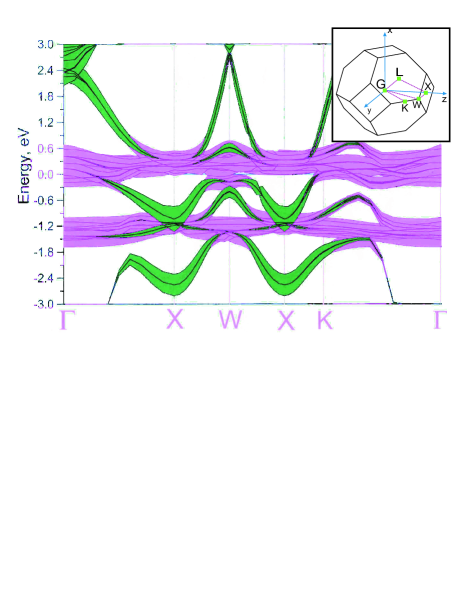
Figure 1: (Color online) Band structure of Cm with indicated contribution of $5f$ (light shade, red online) and $6d$ (dark shade, green online) characters. The layout is chosen to show $d$-contributions over $f$-contribution. Inset: Brillouin zone of $fcc$ structure with indicated high symmetry directions.

In Figure 1 we present LDA band structure of Cm II with the projections of the $5f$- and $6d$- characters. The overwhelming contribution of $f$ character within a $1eV$ window around Fermi level suggests the conclusion that the low-energy physics of actinides is completely controlled by $f-f$ bonding. As we show below this intuitive interpretation turns out to be misleading and Hubbard model alone can not be considered as the low-energy Hamiltonian for actinides. One has to account for presence of $spd$-characters at the Fermi level through the hybridization. Moreover, the hybridization energy scale in actinides turns out to be larger than the average $f-f$ hopping.

III.1 Determining a robust basis for the actinides

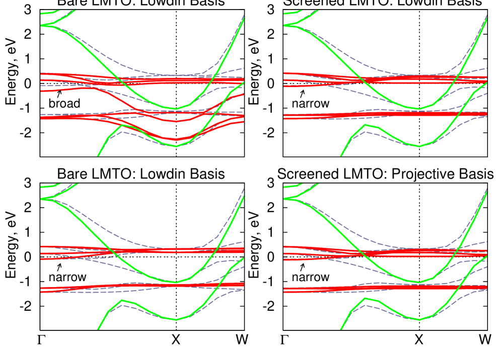
Figure 2: (Color online) Basis difference for fcc Curium. In all panels dashed grey lines represent the LDA band structure , solid light shade lines (green online) represent bands for the block $H_{spd}$ , and solid dark shade line (red online) represent bands for the block $H_{f}$.

In order to determine the optimum basis, we need to define a criteria to judge the different bases. When performing DMFT calculations, one accounts only for a subset of local electronic correlations (those on the $f$ orbital). Therefore, from the perspective of DMFT it is best to have $f$ orbitals with the largest on-site Coulomb repulsion $U$ indranil . A simpler criteria, in the same spirit, is to search for the smallest value of $t^{f}$. We first investigate $t^{f}$ in Cm for the four different basis sets in Table 1. The hybridization $V$ in the Hamiltonian (1) may be set to zero. What remains are the two blocks $H_{f}$ and $H_{spd}$ which are now completely decoupled. The Hamiltonian may now be diagonalized resulting in distinct $spd$ and $f$ bands, and any dispersion of the $f$ bands is due to $t^{f}$. We begin by analyzing the bare LMTOs orthogonalized with the Löwdin procedure (see top left panel Figure 2). Some $f$ bands have a dispersion greater than $1.5eV$ which is unfavorable. Using the bare LMTOs orthogonalized with the projective procedure, the $f$ bands are far more narrow with a width of less than $0.4eV$ (see left bottom panel of Figure 2). In this case the two sets of bands can be identified as $S=\frac{7}{2}$ and $S=\frac{5}{2}$. The Löwdin orthogonalization mixes the $spd$ states into the $f$ states which causes a larger dispersion and a mixing of $f$ bands between the $S=\frac{7}{2}$ and $S=\frac{5}{2}$ states. Alternatively, the projective orthogonalization minimizes the amount of $spd$ character in the $f$ states which results in weakly dispersing $f$ states.

The same exercise can be performed using the screened LMTOs (see right top and bottom panels of Figure 2). In this case, both the Löwdin and the projective orthogonalization produce nearly identical results to the projective orthogonalization of the bare LMTOs. The screened LMTOs are insensitive to the method of orthogonalization due to the fact that orbitals are already well localized with a well-defined character. In conclusion, one may use bare LMTOs orthogonalized with the projective procedure or screened LMTOs orthogonalized in an arbitrary manner as a robust basis for the actinides.

III.2 Decomposition of the actinide band structures

Having established a sensible basis for the actinides, we choose to proceed with projective orthogonalization of bare LMTOs. It is instructive to zero the hybridization $V$ of the Hamiltonian for U, $\alpha$-Pu, $\delta$-Pu, and Cm, and to compare the full band structure with the $spd$ and $f$ bands (see Figures 3 and 4). The same generic behavior can be seen in all four systems. The $spd$ bands have a strong dispersion and cross the Fermi energy in all cases, and the $f$ bands are relatively narrow. The fact that the $spd$ bands cross the Fermi energy in all cases is a critical point which indicates that there will be $spd$ states at the Fermi energy even if the $f$ states become completely localized. When the hybridization $V$ is switched on, the $f$ and $spd$ bands interact via $V$ and mix. Therefore the strength of $V$ can qualitatively be seen as the difference between the full DFT bands and the $f$+$spd$ bands. The $f$ bands are relatively wide for Uranium and become increasingly narrow as Curium is approached. The $spd$ bands follow the same general trend, but the relative changes are smaller. The values of $V$ and $t^{f}$ will be quantified below.

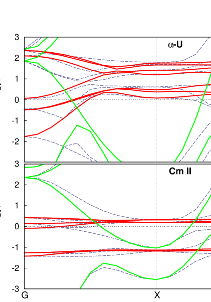
Figure 3: (Color online) Band structure of $\alpha$-U (top) and Cm II (bottom). Grey dashed lines represent LDA bands, solid light shade lines (green online) represent bands of $H_{spd}$, and solid dark shade lines (red online) represent bands of $H_{f}$.

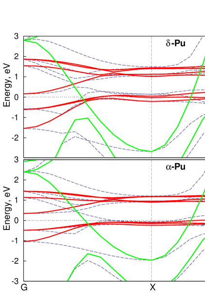
Figure 4: (Color online) Band structure of $\alpha$-Pu (top) and $\delta$-Pu(bottom). Grey dashed lines represent LDA bands, solid light shade lines (green online) represent bands of $H_{spd}$, and solid dark shade lines (red online) represent bands of $H_{f}$.

III.3 Quantitative analysis of $V$ and $t^{f}$

In order to quantify $V$ and $t^{f}$ for the different actinides, we introduce an average $V$ and $t^{f}$ so each actinide may be characterized by two numbers.

First, we recall that the Hamiltonian (1) consist of four blocks:

$$H(\mathbf{k})=\left(\begin{array}[]{cc}H^{spd}(\mathbf{k})&V_{\mathbf{k}}\\ V_{\mathbf{k}}^{\dagger}&H^{f}(\mathbf{k})\\ \end{array}\right)$$ (37)

Then the average strength of the hybridization per band is defined as follows:

$$\overline{V}=\frac{1}{N_{f}}[\frac{1}{2}\emph{Tr}\langle\tilde{H}(\mathbf{k})\tilde{H}(\mathbf{k})\rangle]^{1/2},$$ (38)

where $\tilde{H}(\mathbf{k})$ stands for hamiltonian (37) with $H_{spd}(\mathbf{k})=H_{f}(\mathbf{k})=0$, $N_{f}=14$ stands for number of $f$-bands, and $\langle\ldots\rangle=\frac{1}{N_{\mathbf{k}}}\sum_{\mathbf{k}}\ldots$ . The definition (38) was chosen to match hybridization $V$ of standard Anderson model in two-band limit.

The average value of $t^{f}$ is defined as follows:

$$\overline{t^{f}}=\frac{1}{N_{f}}[\emph{Tr}(\langle H_{f}(\mathbf{k})^{2}\rangle-\langle H_{f}(\mathbf{k})\rangle^{2})]^{1/2},\\$$ (39)

and matches $t^{f}$ of the canonical Hubbard model in the limit of one-band model.

Table  3 lists the calculated values of the average hybridization $\overline{V}$ and $\overline{t^{f}}$ and the average energy for the $j=5/2$ and $j=7/2$ levels of the $f$ manifold relative to the Fermi energy. The averages are generally the same for the bare and screened LMTOs, with the exception of the average hybridization being slightly larger in the case of screened LMTOs.

Table 3: Quantitative characteristics for actinide series (in eV).

	$\overline{V}$	$\overline{t^{f}}$	$\overline{V}/\overline{t^{f}}$	$\epsilon_{5/2}-\mu$	$\epsilon_{7/2}-\mu$
Bare LMTO
$\alpha$-U	0.483	0.188	2.569	0.442	1.353
$\alpha$-Pu	0.423	0.146	2.897	-0.180	0.971
$\delta$-Pu	0.305	0.099	3.081	-0.129	1.008
Cm II	0.189	0.050	3.780	-1.152	0.238
Screened LMTO
$\alpha$-U	0.490	0.188	2.606	0.444	1.355
$\alpha$-Pu	0.429	0.146	2.938	-0.178	0.973
$\delta$-Pu	0.309	0.098	3.153	-0.128	1.009
Cm II	0.192	0.050	3.840	-1.151	0.238

Table 4: Nearest Neighbors contributions to $\overline{V}$ and $\overline{t^{f}}$ (in eV).

	$\overline{V}_{n}$	$\overline{t^{f}_{n}}$	$\overline{V_{n}}/\overline{t^{f}_{n}}$
$\alpha$-U	0.371	0.172	2.157
$\alpha$-Pu	0.324	0.134	2.418
$\delta$-Pu	0.232	0.090	2.578
Cm II	0.143	0.045	3.178

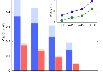
Figure 5: (Color online) Histogram represents average hybridization (first bar for each element, blue online) and average $f-f$ hopping (second bar for each element, red online) as functions of atomic number. The shadow bars show $\overline{V}$ and $\overline{t^{f}}$ for the original Hamiltonian and bright bars represent values $\overline{V}_{n}$ and $\overline{t^{f}_{n}}$ arising from nearest neighbors contributions only. In inset: the ratio $\overline{V}/\overline{t^{f}}$ (squares) as function of atomic number. The ratio of nearest neighbor contributions is represented by circles.

These results are displayed graphically in Figure 5. In all cases, $\overline{V}$ is significantly greater than $\overline{t^{f}}$. As one moves along actinides series from U to Cm $\overline{t^{f}}$ decreases as much as four times. The average value of hybridization $\overline{V}$ also decreases but at a slower rate, as indicated by the inset plot of the ratio of $\overline{V}$ and $\overline{t^{f}}$. The strong decrease in $\overline{V}$ and $\overline{t^{f}}$ will both contribute to the localization of the $f$ states. In order to determine if the localization could be predominantly assigned to either Mott or Anderson character, explicit many-body calculations such as DMFT would need to be performed.

In order to provide further insight into the degree of locality of the basis, it is instructive to determine the fraction of $\overline{V_{n}}$ and $\overline{t^{f}_{n}}$ which arise solely from nearest-neighbor hopping. The corresponding values are presented in Table 4 and can also be seen in Figure 5. First nearest neighbors contribute $\approx 75\%$ to $\overline{V}$ and $\approx 90\%$ to the $\overline{t^{f}}$. The ratio of $\overline{V_{n}}/\overline{t^{f}_{n}}$ is also given for the nearest-neighbor contribution, and the shape and slopes of the two respective curves are very similar. This analysis indicates that nearest-neighbor hopping in real space accounts for most of the relevant one-electron physics.

III.4 Real space analysis of band structure

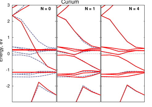
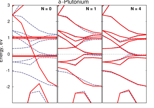
Figure 6: (Color online) Band structure of Curium (top) and $\delta$-Pu (bottom) when N nearest neighbors are taken into account for $f$-orbitals (red solid line) is compared to original LDA bands (dashed grey line). The band structures are plotted for $\Gamma$-$X$ direction.

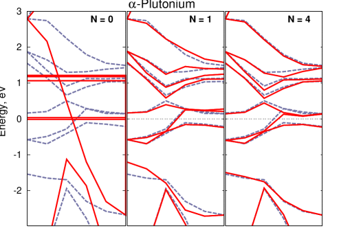
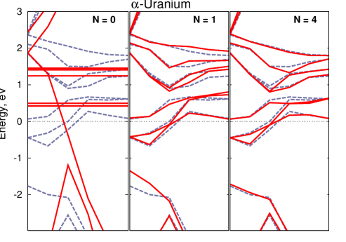
Figure 7: (Color online) Band structure of $\alpha$-Pu (top) and $\alpha$-U (bottom) when N nearest neighbors are taken into account for $f$-orbitals (red solid line) is compared to original LDA bands (dashed grey line). The band structures are plotted for $\Gamma$-$X$ direction.

In the above analysis it was shown that nearest-neighbor hopping accounts for a strong majority of $\overline{V}$ and $\overline{t^{f}}$. Therefore, it is suggestive that the one-electron bands can be reproduced with relatively short ranged hoppings $t^{f}$ and $V$. In order to determine the degree of locality, we plot the band structure as a function of the number of neighbors for the $t^{f}$ and $V$ hoppings (see Figures 6 and 7). Results are given for zero, one, and fourth neighbor hopping. The hopping $t^{spd}$ are not truncated as it is clear they will definitely have relatively long-range hoppings. The generic results are similar for all four materials. The case with zero neighbors results in flat bands having the on-site energy of each orbital. When first nearest-neighbors are included the resulting bands are an excellent approximation to the full band structure. Including up to four nearest-neighbors yields nearly perfect agreement. Cm has better agreement than U for a given number of nearest-neighbors, and this reflects the larger degree of localization in the late actinides as compared to the early actinides. In conclusion, the band structure of the actinides is dominated by nearest-neighbor hopping when using an appropriate basis.

III.5 Conclusion

In summary, a one-electron analysis of band structure of the actinides was presented. We demonstrated that bare LMTOs orthogonalized with the projective method and screened LMTOs are robust bases, in the sense that they give rise to $f$ orbitals with minimal hopping. Analysis of the Hamiltonian in these bases yielded a number of interesting results. When switching off the hybridization $V$, it was shown that the $spd$ states cross the Fermi energy and hence will be present at the Fermi energy even if the $f$ electrons become localized. Our description is in reasonable agreement with the earlier work of HarrisonHarrison83 . In particular, the matrix elements of spin-orbit coupling indeed have atomic-like nature and the hybridization is much larger than the direct $f-f$ hopping Harrison83 . However the $spd$ bands are not simple plane waves and the hybridization matrix element does not have a simple $\mathbf{k}$-dependence proportional to an $l=2$ spherical harmonic.

Evaluation of the average hybridization $\overline{V}$ and average $f-f$ hopping $\overline{t^{f}}$ as a function of the actinides showed that both quantities decrease strongly. The quantity $\overline{t^{f}}$ decreased faster than $\overline{V}$, but $\overline{V}$ was larger in all actinides. Hence, the Anderson model of the localization-delocalization transition, rather than a multiorbital Hubbard model is needed to describe the physics of the actinides once explicit many-body calculations are added. This is the point of view taken in recent DMFT work Shim2006 , and no further reduction to a model containing only f bands seems possible. Finally, a real-space analysis of the band structure demonstrated that nearest-neighbor hopping accounts for most of the band structure in the basis used in this study, thus providing a tight binding fitting of the bands of the actinides that can be useful in further studies.

Appendix A Green’s function in the projective base

In the DMFT approach one needs to choose a set of localized Wannier states in which correlations are strongest. In the context of actinides, the orbitals with the largest component of $5f$ character are the appropriate set of orbitals.

For many-body calculations, it is convenient if the set of localized orbitals is orthogonal. In this case, it is desired that the local Green’s function is connected to the partial density of states by the usual relation

$$D^{l}_{mm^{\prime}}(\omega)\approx\frac{1}{2\pi i}(\widetilde{G}^{\dagger}_{loc}-\widetilde{G}_{loc})_{lm,lm^{\prime}}.$$ (40)

In another words, the localized set of orbitals need to give rise to the $5f$ spectra defined by

$$D^{l}_{mm^{\prime}}(\omega)=\int\frac{d\mathrm{r}_{1}d\mathrm{r}_{2}}{2\pi i}Y_{lm}^{*}(\hat{\mathrm{r}}_{1})(G^{\dagger}(\mathrm{r}_{1},\mathrm{r}_{2})-G(\mathrm{r}_{1},\mathrm{r}_{2}))Y_{lm^{\prime}}(\hat{\mathrm{r}}_{2})$$ (41)

with $l=3$ for actinides. Only in this case, the number of $f$ electrons (or the valence of the material) is connected to the impurity $f$ count, as obtained in the DMFT calculation.

Using the LMTO basis set Eq. (12), the partial density of states becomes

$$D^{l}_{mm^{\prime}}(\omega)=\frac{1}{2\pi i}\sum_{\mathbf{k}}\left\{(G_{\mathbf{k}\omega}^{\dagger}-G_{\mathbf{k}\omega})o^{HH}-[S_{\mathbf{k}}(G_{\mathbf{k}\omega}^{\dagger}-G_{\mathbf{k}\omega})]o^{HJ}-[(G_{\mathbf{k}\omega}^{\dagger}-G_{\mathbf{k}\omega})S_{\mathbf{k}}^{\dagger}]o^{JH}+[S_{\mathbf{k}}(G_{\mathbf{k}\omega}^{\dagger}-G_{\mathbf{k}\omega})S_{\mathbf{k}}^{\dagger}]o^{JJ}\right\}_{lm,lm^{\prime}}$$ (42)

where the momentum dependent Green’s function is

$$G_{\mathbf{k}\omega}=(O_{\mathbf{k}}(\omega+\mu)-H_{\mathbf{k}}-\Sigma_{\mathbf{k}\omega})^{-1}$$ (43)

and overlap numbers $o^{AB}$ are defined by Eq. (28).

The projective orthogonalization Eq. (34) leads to the following Green’s function

$$\widetilde{G}_{\mathbf{k}\omega}=(T_{\mathbf{k}}^{\dagger}[O_{\mathbf{k}}(\omega+\mu)-H_{\mathbf{k}}-\Sigma_{\mathbf{k}\omega}]T_{\mathbf{k}})^{-1}$$ (44)

$$=(\mathcal{H}-\mathcal{J}S_{\mathbf{k}})G_{\mathbf{k}\omega}(\mathcal{H}-\mathcal{J}S_{\mathbf{k}})^{\dagger}.$$ (45)

The local spectral function in this new base therefore becomes

$$\frac{1}{2\pi i}(\widetilde{G}^{\dagger}_{loc}-\widetilde{G}_{loc})_{lm,lm^{\prime}} = \frac{1}{2\pi i}\sum_{\mathbf{k}}\left\{[G^{\dagger}_{\mathbf{k}\omega}-G_{\mathbf{k}\omega}]_{LL^{\prime}}\mathcal{H}_{l}^{*}\mathcal{H}_{l}-[S_{\mathbf{k}}(G_{\mathbf{k}\omega}^{\dagger}-G_{\mathbf{k}\omega})]_{LL^{\prime}}\mathcal{H}_{l}^{*}\mathcal{J}_{l}\right.$$ (46)

$$\left.\quad-[(G^{\dagger}_{\mathbf{k}\omega}-G_{\mathbf{k}\omega})S_{\mathbf{k}}^{\dagger}]_{LL^{\prime}}\mathcal{J}_{l}^{*}\mathcal{H}_{l}+[S_{\mathbf{k}}(G_{\mathbf{k}\omega}^{\dagger}-G_{\mathbf{k}\omega})S_{\mathbf{k}}^{\dagger}]_{LL^{\prime}}\mathcal{J}_{l}^{*}\mathcal{J}_{l}\right\}$$

which is equivalent to the partial density of state Eq. (42) provided the condition Eq. (31) is satisfied. Extensive experience shows that in the case of localized $d$ and $f$ orbitals, the condition is always satisfied to very high accuracy (better than $1\%$) therefore the relation between the partial density of states and local Green’s function Eq. (40) is also satisfied to high accuracy.

References

- (1) Plutonium Futures - the Science, Conference transactions of the Topical conference on plutonium and actinides, ed. by K. K. S. Pillay, K. C. Kim (Santa Fe, New Mexico, USA, 2000)
- (2) P. Soderlind, O. Eriksson, B. Johansson, J. M. Wills, and A. M. Boring, Nature (London) 374, 524 (1995).
- (3) S. Heathman, R. G. Haire, T. Le Bihan, A. Lindbaum, M. Idiri, P. Normile, S. Li, R. Ahuja, B. Johansson, and G. H. Lander, Science 309, 110 (2005)
- (4) A. Lindbaum, S. Heathman, K. Litfin, Y. Meresse, R. G. Haire, T. Le Bihan, and H. Libotte, Phys. Rev. B 63, 214101 (2001)
- (5) P. Soderlind and B. Sadigh, Phys. Rev. Lett. 92, 185702 (2004)
- (6) S. Y. Savrasov, G. Kotliar and E. Abrahams, Nature 410, 793 (2001)
- (7) Handbook on the Physics and Chemistry of the Actinides, edited by A. J. Freeman and G. H. Lander ( North-Holland, Amsterdam, 1984).
- (8) J. C. Lashley, A. Lawson, R. J. McQueeney, and G. H. Lander, Phys. Rev. B 72, 054416 (2005)
- (9) H. L. Skriver, O. K. Andersen and B. Johansson, Phys. Rev. Lett. 41, 42(1978)
- (10) O. Eriksson, J. D. Becker, A. V. Balatsky, and J. M. Wills, Journal of Alloys and Compounds 287, 1 (1999)
- (11) B. Johansson, Philos. Mag. 30, 469 (1974).
- (12) B. Johansson, Phys. Rev. B 11, 2740 (1975)
- (13) J. van Ek, P. A. Sterne, and A. Gonis, Phys. Rev. B 48, 16 280(1993)
- (14) M. D. Jones, J. C. Boettger, R. C. Albers, and D. J. Singh, Phys. Rev. B 61, 4644 (2000)
- (15) P. Söderlind, J. M. Wills, B. Johansson, and O. Eriksson, Phys. Rev. B 55, 1997 (1997)
- (16) A. Svane, L. Petit, Z. Szotek, and W. M. Temmerman, arXiv:cond-mat/0610146v2
- (17) S. Y. Savrasov and G. Kotliar, Phys. Rev. Lett. 84, 3670 (2000)
- (18) A. O. Shorikov, A. V. Lukoyanov, M. A. Korotin, and V. I. Anisimov, Phys. Rev. B 72, 024458 (2005)
- (19) A. B. Shick, V. Drchal, and L. Havela, Europhys. Lett. 69, 588 (2005)
- (20) J. H. Shim, K. Haule, G. Kotliar, Nature 446, 513-516 (2007).
- (21) Jian-Xin Zhu, A. K. McMahan, M. D. Jones, T. Durakiewicz, J. J. Joyce, J. M. Wills and R. C. Albers, arXiv:cond-mat/0705.1354
- (22) L. V. Pourovskii, G. Kotliar, M. I. Katsnelson, and A. I. Lichtenstein, Phys. Rev. B 75, 235107 (2007)
- (23) (see for review and references therein) V. I. Anisimov, A. O. Shorikov, and J. Kuneš, J. Alloys Compd. (2006), doi:10.1016/j.jallcom.2006.10.150
- (24) K. Held, C. Huscroft, R. T. Scalettar, and A. K. McMahan, Phys. Rev. Lett. 85, 373 (2000)
- (25) L. de’ Medici, A. Georges, G. Kotliar, and S. Biermann, Phys. Rev. Lett. 95, 066402 (2005)
- (26) W. A. Harrison, Phys. Rev. B 28, 550 (1983)
- (27) W. A. Harrison and G. K. Straub, Phys. Rev. B 36, 2695 (1987)
- (28) M. I. Katsnelson, I. V. Solovyev, ans A. V. Trefilov, JETP Letters 56, 272 (1992)
- (29) L. Severin, Rhys. Rev. B 46, 7905 (1992)
- (30) R. Jullien, E. Galleani d’Agliano, and B. Coqblin, Phys. Rev. B 6, 2139 (1972)
- (31) R. Jullien, and B. Coqblin, Phys. Rev. B 8, 5263 (1972)
- (32) I. V. Solovyev, Phys. Rev. B 73, 155117 (2006)
- (33) H. L. Skriver, The LMTO Method (Springer, Berlin, 1984)
- (34) O. K. Andersen and O. Jepsen, Phys. Rev. Lett. 53, 2571(1984); O. K. Andersen, Z. Pawlowska and O. Jepsen, Phys. Rev. B 34, 5253 (1986)
- (35) P. Löwdin, J. Chem. Phys. 18, 365(1950)
- (36) K. Haule, V. Oudovenko, S.Y. Savrasov, and G. Kotliar, Phys. Rev. Lett. 94, 036401 (2005); K. Haule in preparation.
- (37) I. Turek, V. Drchal, J. Kudrnovsky, M. Sob and P. Weinberger, Electronic Structure of Disordered Alloys, Surfaces and Interfaces (Springer, 1996)
- (38) K. T. Moore, G. van der Laan, R. G. Haire, M. A. Wall, A. J. Schwartz, and P. Söderlind, Phys. Rev. Lett. 98, 236402 (2007); K. T. Moore, G. van der Laan, R. G. Haire, M. A. Wall, and A. J. Schwartz, Phys. Rev. B 73, 033109 (2006); K. T. Moore, M. A. Wall, A. J. Schwartz, B. W. Chung, D. K. Shuh, R. K. Schulze, and J. G. Tobin, Phys. Rev. Lett. 90, 196404 (2003).
- (39) O. K. Andersen, O. Jepsen, and D. Glotzel, Canonical Description of the Band Structures of Metals, Proceedings of the International School of Physics, Course LXXXIX, ”Enrico Fermi” Varenna, edited by F. Bassani, F. Fumi, and M. P. Tosi (North-Holland, Amsterdam, 1985), p. 59
- (40) I. Paul and G. Kotliar, European Physical Journal B: Condensed Matter Physics 51, 189-193 (2006).