Diversity-Multiplexing Tradeoff of Asynchronous Cooperative Diversity in Wireless Networks

Abstract

Synchronization of relay nodes is an important and critical issue in exploiting cooperative diversity in wireless networks. In this paper, two asynchronous cooperative diversity schemes are proposed, namely, distributed delay diversity and asynchronous space-time coded cooperative diversity schemes. In terms of the overall diversity-multiplexing (DM) tradeoff function, we show that the proposed independent coding based distributed delay diversity and asynchronous space-time coded cooperative diversity schemes achieve the same performance as the synchronous space-time coded approach which requires an accurate symbol-level timing synchronization to ensure signals arriving at the destination from different relay nodes are perfectly synchronized. This demonstrates diversity order is maintained even at the presence of asynchronism between relay node. Moreover, when all relay nodes succeed in decoding the source information, the asynchronous space-time coded approach is capable of achieving better DM-tradeoff than synchronous schemes and performs equivalently to transmitting information through a parallel fading channel as far as the DM-tradeoff is concerned. Our results suggest the benefits of fully exploiting the space-time degrees of freedom in multiple antenna systems by employing asynchronous space-time codes even in a frequency flat fading channel. In addition, it is shown asynchronous space-time coded systems are able to achieve higher mutual information than synchronous space-time coded systems for any finite signal-to-noise-ratio (SNR) when properly selected baseband waveforms are employed.

Keywords: asynchronous space-time codes, cooperative diversity, distributed delay diversity, diversity-multiplexing tradeoff, relay channels.

I Introduction

In wireless networks, treating intermediate nodes between the source and its destination as potential relays and utilizing these relay nodes to improve the diversity gain has attracted considerable attention lately and re-kindled interests in relay channels after this problem was first tackled from the perspective of Shannon capacity in the 70’s [1, 2]. One school of works [3, 4, 5] follow the footsteps of [2], where they employ block Markov superposition encoding, random binning and successive decoding as coding strategy. Another line of work adopts the idea of cooperative diversity which was first proposed in [6, 7] for CDMA networks, and then extended to wireless networks with multiple sources and relays [8, 9, 10, 11, 12, 13, 14]. We are not attempting to provide a comprehensive review of all related works on relay channels here [3], but instead divert our attentions to those work related with cooperative diversity.

In this paper, we mainly focus on two well received relaying strategies, namely, decode-and-forward (DF) and amplify-and-forward (AF) schemes. Decision on which relaying strategy is adopted is subject to constraints imposed upon relay nodes. If nodes cannot transmit and receive at the same time and thus work in a half-duplex mode [15], the communication link in a relay channel with a single level of relay nodes consists of two phases. In the first phase, the source broadcasts its information to relays and its destination. During the second phase, relays forward either re-encoded source transmissions (decode-and-forward) or a scaled version of received source signals (amplify-and-forward) [10]. At the destination, signals arriving over two phases are jointly processed to improve the overall performance. Variations of these schemes include allowing source nodes to continuously send packets over two phases to increase the spectral efficiency [12, 16]. As for coding strategies through which cooperative diversity is achieved, [11] proposes to encode the source information over two independent blocks from source to destination and relays to destination, respectively. In [13], without requiring relay nodes to provide feedback messages to the source, rate compatible punctured convolutional codes (RCPC) and turbo codes are proposed to encode over two independent blocks. Also, an extension is made by putting multiple antennas at relay nodes to further improve the diversity and multiplexing gain. If multiple relay nodes are considered as virtual antennas, a space-time-coded cooperative diversity approach is proposed in [9] to jointly encode the source signals across successful relay nodes during the second phase.

As noted in [17], synchronization of relay nodes is an important and critical issue in exploiting cooperative diversity in wireless ad hoc and sensor networks. However, in the existing works, e.g., [18, 9], it has been assumed that relay nodes are perfectly synchronized such that signals arriving at the destination node from distinct relay nodes are aligned perfectly with respect to their symbol epochs. Under this assumption, distributed space-time-coded cooperative diversity approach achieves diversity gains in the order of the number of available transmitting nodes in a relay network [9].

Perfect synchronization is, however, hard, if not impossible, to be achieved in infra-structureless wireless ad-hoc and sensor networks. In [19], the issue of carrier asynchronism between the source and relay node is addressed in terms of its impact on the lower and upper bounds of the outage and ergodic capacity of a three-node wireless relay channel. At the presence of time delays between relay nodes, an extension of Alamouti space-time-block-codes (STBC) [20] is proposed in [21] to exploit spatial diversity when time delay is only an integer number of symbol periods. And in [22, 23], macroscopic space-time codes are designed to perform robust against uncertainties of relative delays between different basestations. Without requiring the symbol synchronization, we propose a repetition coding based distributed delay diversity scheme in [24, 25] which achieves the same order of diversity promised by distributed space-time codes. Unlike the extension of other approaches to the synchronization problem in distributed space-time coding [22], the proposed system also admits a robust and easily trainable receiver when synchronization is not present in the system.

In [26], relay nodes perform adaptive decode-and-forward or amplify-and-forward schemes allowing them to transmit or remain silent depending on the received signal-to-noise-ratio (SNR). However, their proposed schemes require intentionally increasing data symbol period to avoid inter-symbol-interference (ISI) caused by the asynchronous transmission of the same source signal to different receivers, which limits efficiency. In [27], asynchronism caused by phase error of channel fading variables is studied in terms of its impact on relay network’s energy efficiency in low SNR region.

To the best of our knowledge, there does not exist yet too much work regarding the impact of symbol level asynchronism on the performance of relay networks in a comprehensive manner. The system model in [28] is closest to what we assumed in [29, 30] and this paper in terms of the consideration of symbol level asynchronism. However, only AF scheme is considered in [28] from the perspective of the scaling law of ergodic capacity. In this paper, diversity-multiplexing (DM) tradeoff function is adopted as a metric to compare the performance of our proposed asynchronous cooperative diversity schemes with the existing synchronous space-time-coded cooperative diversity strategy. As first put forward by Zheng and Tse in the context of multiple antenna systems [31], the diversity-multiplexing tradeoff function reveals a fundamental relationship between diversity gain which characterizes the asymptotic rate of decoding error approaching zero as SNR increases, and multiplexing gain which characterizes the asymptotic spectral efficiency in the large SNR regime. The idea has recently been extended to relay channels [9, 16] and multiple access channels [32].

Without loss of generality (WLOG), we consider a relay channel where a source node communicates with its destination with the help of two potential relays. Nodes are assumed to work in a half duplex mode [15, 27, 28], in which no one can transmit and receive simultaneously. The entire transmission period is divided into two phases. In the first phase, source broadcasts while relays and destination listen. In the second phase, source stops transmitting and relays which succeed in decoding in the first phase forward source messages to the destination, where received signals over the whole period is jointly processed. Our major contributions can be summarized as follows.

We first show the lower bound of the DM-tradeoff for space-time-coded cooperative diversity scheme developed in [9] is actually the exact tradeoff function. In addition, it is shown the overall DM-tradeoff under the decode-and-forward strategy is dominated by a bottleneck case when no relay node succeeds in decoding the source information correctly.

We then propose two asynchronous cooperative schemes under the symbol-level asynchronism. The first one is distributed delay diversity scheme in which successful relay nodes forward source information encoded with the same codewords. Consequently, an equivalent multipath fading channel is constructed between relays and destination. When relay codeword is independent of source codeword, we prove that the overall DM-tradeoff function remains unchanged compared with the synchronous scheme, provided the MAC protocol ensures the relative delay $T_{0}$ between two relay-destination links satisfies $T_{0}\geq 2/B_{w}$, where $B_{w}$ is the bandwidth of baseband signals. When relay codeword are identical with the source codeword, only when $B_{w}T_{0}$ is a positive integer, can we reach the same conclusion as the independent case. Otherwise, the overall DM-tradeoff is degraded.

The second asynchronous cooperative diversity approach we propose is more bandwidth efficient in that asynchronous space-time codes are employed across successful relay nodes to jointly encode the decoded source information at the presence of asynchronism. We first prove this scheme achieves the same amount of overall diversity as the synchronous one. Moreover, we demonstrate the presence of asynchronism provides us an opportunity to fully exploit all degrees of freedom in space-time domain, as evidenced by an improvement of the DM-tradeoff when all relay nodes succeed in decoding in the first phase. Such an improvement is due to the decoupling of the original multiple-input-single-output (MISO) channel between relay nodes and destination into an equivalent parallel channel whose DM-tradeoff is better than that of a synchronous MISO channel. In addition, under certain conditions on baseband waveforms, the mutual information of the asynchronous channel is even higher than the synchronous channel for any finite SNR.

It has been recently shown in [16] that the spectral efficiency and DM-tradeoff for relay channels can be improved if a source node keeps on transmitting signals over two phases and relay nodes don’t start forwarding until they collect sufficient information and energy to perform the decoding. As a comparison, we propose a mixing approach where the amplify-and-forward and asynchronous decode-and-forward schemes are combined together. Such an approach not only alleviates to some extent the bottleneck caused by the absence of successful relay nodes, but also yields a better DM-tradeoff than schemes proposed [16] for some range of multiplexing gain even when the source only broadcasts in the first phase and stops its transmission in the second phase, which is suggested not efficient in [16]. Our results suggest the ultimate efficient relaying strategy should be featuring both the non-orthogonal channel allocation as proposed by [16], as well as the complete exploitation of temporal-spatial degrees of freedom using asynchronous coding approach as revealed in our analysis.

This paper is organized as follows. The system model of a relay channel is introduced in Section II. We revisit the DM-tradeoff of the synchronous space-time-coded scheme proposed by [9] in Section III-A and prove their lower bound is actually the exact value. An independent coding based and repetition coding based distributed delay diversity schemes and an asynchronous space-time coded cooperative diversity scheme are proposed in Section III-B and  III-C, respectively. Their DM-tradeoff are analyzed and compared against the synchronous coded approach. A mixing relaying strategy combining DF and AF is proposed in Section III-D to resolve to certain extent the bottleneck issue which restricts the overall DM-tradeoff for orthogonal relay channels. Finally, we conclude the paper in Section IV.

II System Model

Figure 1: System model of an ad hoc wireless network

To simplify analysis and reveal fundamental insights, we consider a relay network where a source node transmits messages to its destination node with the help of $K=2$ relays. It is assumed relay nodes work in a half-duplex mode, which prohibits them from transmitting and receiving at the same time [15]. As assumed in [9], the system works in two phases. In the first phase, the source broadcasts its transmission to its destination and potential relays. In the second phase, the source remains silent and only those relays which succeed in decoding the source information forward the packets after reprocessing. A mathematical model of such a network is shown in Figure 1.

After some processing of the received signal $Y_{R_{k}}(t),k=1,2$ from the source node $N_{S}$ at the $k$th relay node $N_{R_{k}}$, $N_{R_{k}}$ transmits the processed packets via $X_{R_{k}}(t)$ to the destination node $N_{D}$, where signals from all involved paths are processed jointly. Quasi-static narrow-band transmission is assumed where the channel between any pair of nodes is frequency non-selective, and the associated fading coefficients remain unchanged during the transmission of a whole packet, but are independent from node to node and packet to packet. Time delays $\{\tau_{k}\}$ are introduced on each path, which incorporate the processing time at relay nodes and propagation delays of the whole route. More specifically, $\tau_{0}$ is the delay from $N_{S}$ to $N_{D}$, and $\tau_{k}$ is the cumulative delay for the transmission from $N_{S}$ to $N_{R_{k}}$, processing at $N_{R_{k}}$ and for transmission from $N_{R_{k}}$ to $N_{D}$, for $k=1,2$.

The noise processes $W_{S}(t)$, $W_{D}(t)$ and $W_{k}(t),k=1,2$ are independent complex white Gaussian noise with two-sided power spectral density ${\cal N}_{0}$. Assume signals $X_{i}(t),i\in\left\{S,R_{1},R_{2}\right\}$ share a common radio channel with complex baseband equivalent bandwidth $[-B_{w}/2,B_{w}/2]$ and each node transmits signals of duration $T_{d}$, which leads to the transmission of $L=\lfloor B_{w}T_{d}\rfloor$ independent complex symbols over one packet. Define $\mbox{SNR}\stackrel{{\scriptstyle\Delta}}{{=}}\frac{P_{s}}{{\mathcal{N}_{0}}B_{w}}=\frac{\hat{P}_{s}}{{\mathcal{N}}_{0}}$, where $P_{s}$ and $\hat{P}_{s}=P_{s}/B_{w}$ are the common continuous and discrete time transmission power of each transmitting node, respectively [9], which are assumed fixed.

The complex channel gain $\alpha_{i,j}$ captures the effects of both pathloss and quasi-static fading on links between node $N_{i}$ and node $N_{j}$, where $i\in\left\{S,R_{1},R_{2}\right\}$, and $j\in\left\{R_{1},R_{2},D\right\}$. Statistically, $\alpha_{i,j}$ are modeled as zero mean, mutually independent complex Gaussian random variables with variances $\sigma^{2}_{i,j}$. The fading variances are specified using wireless path-loss models based on the network geometry [33]. Here, it is assumed that $\sigma^{2}_{i,j}\propto 1/d^{\mu}_{i,j}$, where $d_{i,j}$ is the distance from node $N_{i}$ to $N_{j}$, and $\mu$ is a constant whose value, as estimated from field experiments, lies in the range $2\leq\mu\leq 5$. Throughout this paper, we assume $\alpha_{i,j}$ is perfectly known at receiver $N_{j}$, but not available to the transmitter $N_{i}$. Consequently, transmission schemes exploiting transmitter side channel state information (CSI), such as successive encoding [34] using dirty paper coding approach [35] and power control schemes [36] , are not considered in this paper.

The two-phase transmission and half-duplex mode of relay nodes results in orthogonality in time between the packet arriving at $N_{D}$ via the direct path from $N_{s}$ and the collection of packets arriving at $N_{D}$ through different relay nodes. Note that the orthogonality between signals $X_{R_{1}}(t)$ and $X_{R_{2}}(t)$ is not assumed, which forms the crux of the problem. Time difference $\tau_{k}-\tau_{0}$ incorporates the processing time of a whole packet at $N_{R_{k}}$ in addition to the relative propagation delay between the $k$th relay path and the direct link. Without loss of generality (WLOG), $\tau_{0}$ is set to zero. Under the preceding model, the received signals in Fig. 1 are specified by :

$$Y_{R_{k}}(t)=\alpha_{S,R_{k}}X_{S}(t)+W_{k}(t),\,k=1,2,$$

$$Y_{D_{s}}(t)=\alpha_{S,D}X_{S}\left(t\right)+W_{S}(t),$$

$$Y_{D_{R}}(t)=\sum_{j\in{\mathcal{D}}(s)}\alpha_{j,D}X_{j}\left(t-\tau_{j}\right)+W_{D}(t),$$ (1)

where $Y_{D_{s}}(t)$ and $Y_{D_{R}}(t)$ have no common support in time domain, and ${\mathcal{D}}(s)$ denotes the set of relay nodes which have successfully decoded the information from $N_{s}$, whose cardinality $|{\mathcal{D}}(s)|$ satisfies $|{\mathcal{D}}(s)|\in\left\{0,1,2\right\}$.

III Diversity-Multiplexing Tradeoff

III-A Synchronous Distributed Space-time-Coded Cooperative Diversity

The DM-tradeoff of the distributed space-time-coded cooperative relaying proposed in [9] is revisited in this section. To study DM-tradeoff function, the source transmission rate $R$(bits/second/Hz) needs to be parameterized as a function of the transmission SNR as follows [9],

$$R\left(\mbox{SNR}\right)=r\log\left(1+\mbox{SNR}\sigma^{2}_{S,D}\right),$$ (2)

where $0<r\leq 1$ characterizes the spectral efficiency normalized by the direct link channel capacity, which illustrates how fast the source data rate varies with respect to SNR and is defined as the multiplexing gain in [31], i.e.

$$r=\lim_{\small\mbox{SNR}\rightarrow\infty}\frac{R\left(\mbox{SNR}\right)}{\log\mbox{SNR}}.$$

A fundamental figure introduced in [31] is the diversity-multiplexing tradeoff which illuminates the relationship between the reliability of data transmissions in terms of diversity gain, and the spectral efficiency in terms of multiplexing gain. This relationship can be characterized by mapping the diversity gain as a function of $r$, i.e. $d(r)$, where $d(r)$ is the diversity gain and defined by

$$d(r)=\lim_{\mbox{SNR}\rightarrow\infty}-\frac{\log\left(\mbox{Pr}\left[I<R\left(\mbox{SNR}\right)\right]\right)}{\log\mbox{SNR}},$$ (3)

where $I$ is the mutual information between the source and its destination node.

Laneman and Wornell developed lower and upper bounds of this tradeoff function for space-time-coded cooperative diversity scheme by assuming perfect symbol-level synchronization [9]. Denote $d_{stc}(r)$ as the corresponding tradeoff function. The bounds of $d_{stc}(r)$ are

$$(K+1)(1-2r)\leq d_{stc}(r)\leq(K+1)\left(1-\frac{K}{K+1}\cdot 2r\right),$$ (4)

where $K+1$ denotes the total number of potential transmitting nodes in the network. In this paper, we have $K+1=3$ for a four-node network. When $d_{stc}(r)$ is computed using the definition of (3), $\mbox{Pr}\left[I<R\left(\mbox{SNR}\right)\right]$ is the outage probability that the mutual information of an equivalent channel between the source and its destination is below the parameterized spectral efficiency $R$ when all possible outcomes of relays decoding source signals are counted. Next, we show the lower bound $3-6r$ in (4) is actually tight.

Theorem 1

The lower bound of the diversity-multiplexing tradeoff for the synchronous space-time-coded cooperative diversity developed in [9] is tight, i.e. $d_{stc}(r)=(K+1)(1-2r)$.

Proof:

For comparison purpose, similar definitions as in [9] are adopted in the sequel. It will be shown below that a bottleneck case dominates the overall diversity order $d_{stc}(r)$ and thus leads to the desired result.

Suppose identically and independently distributed (i.i.d) circularly symmetric, complex Gaussian codebooks are employed by the source and all successful relay nodes. Conditioned on the decoding set $\mathcal{D}(s)$, the mutual information $I_{stc}$ between $N_{S}$ and $N_{D}$ of the distributed space-time-coded scheme with perfect synchronization is [9, Eq. (18)]

$$I_{stc}=\frac{1}{2}\log\left(1+\frac{2}{K+1}\mbox{SNR}\left|\alpha_{S,D}\right|^{2}\right)+$$

$$\frac{1}{2}\log\left(1+\frac{2}{K+1}\mbox{SNR}\sum_{R_{k}\in{\mathcal{D}(s)}}\left|\alpha_{R_{k},D}\right|^{2}\right),$$ (5)

where $2/(K+1)$ is a normalization factor introduced to make a fair comparison with the non-cooperative scheme and the factor $1/2$ in front of $\log$-functions is due to the encoding over two independent blocks.

The outage probability can be calculated based on the total probability law

$$\mbox{Pr}\left[I_{stc}<R\right]=\sum_{{\mathcal{D}}(s)}\mbox{Pr}\left[{\mathcal{D}}(s)\right]\mbox{Pr}\left[I_{stc}<R|{\mathcal{D}}(s)\right],$$ (6)

where the probability of the decoding set is

$$\mbox{Pr}\left[{\mathcal{D}}(s)\right]=\prod_{R_{k}\in{\mathcal{D}}(s)}\mbox{Pr}\left[I_{S,R_{k}}\geq R\right]\times\prod_{R_{j}\not\in{\mathcal{D}}(s)}\mbox{Pr}\left[I_{S,R_{j}}<R\right],$$ (7)

and $I_{S,R_{j}}$ is the mutual information between $N_{s}$ and $N_{R_{j}}$ using i.i.d complex Gaussian codebooks, and is given by

$$I_{S,R_{j}}=\frac{1}{2}\log\left(1+\frac{2}{K+1}\mbox{ SNR}\left|\alpha_{S,R_{j}}\right|^{2}\right).$$ (8)

In order to derive the overall tradeoff function $d_{stc}(r)$, we need to study the asymptotic behavior of all sum terms in (6) where $R$ should be replaced by (2). However in [9], the bounds of $d_{stc}(r)$ in (4) are developed by first fixing $R$ in order to obtain an asymptotic equivalence form of $\mbox{Pr}\left[I_{stc}<R\right]$ and then substituting the rate $R$ with $R({\mbox{S}NR})$. This approach conceals the dominance of the worst situation when all relay nodes fail in decoding source messages, which consequently drags down the overall diversity order in an overwhelming manner. This point will be made more clearly through our asymptotic analysis.

Consider first the outage probability $\mbox{Pr}\left[I_{S,R_{j}}<R\right]$ for large SNR:

$$\mbox{Pr}\left[I_{S,R_{j}}<R\right]=\mbox{Pr}\left[\frac{1}{2}\log\left(1+\frac{2}{K+1}\mbox{SNR}|\alpha_{S,R_{j}}|^{2}\right)<\right.$$

$$\left.r\log\left(1+\mbox{SNR}\sigma^{2}_{S,D}\right)\right]$$

$$\sim\mbox{Pr}\left[|\alpha_{S,R_{j}}|^{2}<\mbox{SNR}^{2r-1}\frac{\left(\sigma_{S,D}^{2}\right)^{2r}}{2/(K+1)}\right]$$

$$=1-\exp\left\{-\lambda_{S,R_{j}}\mbox{SNR}^{2r-1}c_{0}\right\},$$ (9)

where “$\sim$" is the symbol representing an asymptotic equivalence at large SNR [37], i.e. as $\mbox{SNR}\rightarrow\infty$, $f(\mbox{SNR})\sim g(\mbox{SNR})$ $\Rightarrow\lim_{{\mbox{SNR}}\rightarrow\infty}f(\mbox{SNR})/g(\mbox{SNR})=1$. With $c_{0}=\frac{\left(\sigma_{S,D}^{2}\right)^{2r}}{2/(K+1)}$, the second equality is because $|\alpha_{i,j}|^{2}$ is exponentially distributed with parameter $\lambda_{i,j}=1/\sigma_{i,j}^{2}$. It can be seen from (III-A) that if $r\geq 1/2$, the probability of no successful relay nodes, i.e. $|{\mathcal{D}}(s)|=0$, is in an order of a non-zero constant for large SNR. In addition, the conditional overall outage probability given $|{\mathcal{D}}(s)|=0$ can be determined similarly by

$$\mbox{Pr}\left[I_{stc}<R||{\mathcal{D}}(s)|=0\right]\sim 1-\exp\left\{-\lambda_{S,D}\mbox{SNR}^{2r-1}c_{0}\right\},$$ (10)

which is also in the order of a non-zero constant when $r\geq 1/2$. Therefore, if $r\geq 1/2$, the overall outage probability $\mbox{Pr}\left[I_{stc}<R\right]$ is dominated by a non-zero and non-vanishing term as $\mbox{SNR}\rightarrow\infty$ which is of no interest to our investigation of the DM-tradeoff. Actually, such limitation imposed on multiplexing gain is due to our restriction of letting source and relay nodes work in the half duplex mode. Recently, cooperative diversity schemes addressing this half duplex limitation are proposed in [16]. In Section III-D, we will make comparisons between our proposed strategies and those in [16] to illustrate benefits of exploiting asynchronism. For schemes proposed subsequently in this paper, we only consider multiplexing gains $r\in[0,1/2)$. Under such condition and $e^{x}\sim 1+x$ for $x\rightarrow 0$, we obtain

$$\mbox{Pr}\left[I_{S,R_{j}}<R\right]\sim\lambda_{S,R_{j}}c_{0}\mbox{SNR}^{-(1-2r)},$$ (11)

for $0\leq r<1/2,\,j=1,2$.

Thus, the probability of the decoding set $\mathcal{D}(s)$ is

$$\mbox{Pr}\left[{\mathcal{D}}(s)\right]\sim\left[c_{0}\mbox{SNR}^{-(1-2r)}\right]^{K-|{\mathcal{D}}(s)|}\prod_{j\not\in{\mathcal{D}}(s)}\lambda_{S,R_{j}},$$ (12)

where $|{\mathcal{D}}(s)|\in\left\{0,1,2\right\}$.

Combining (10) and (12), we obtain

$$\mbox{Pr}\left[I_{stc}<R,\,|{\mathcal{D}}(s)|=0\right]\sim\lambda_{S,D}\prod_{j=1}^{2}\lambda_{S,R_{j}}c_{0}^{3}\cdot\mbox{SNR}^{-3(1-2r)}.$$ (13)

Next, we show when $|\mathcal{D}(s)|>0$, the overall diversity is dominated by the term $3(1-2r)$, i.e. $\mbox{SNR}^{-3(1-2r)}$ becomes the slowest vanishing term as $\mbox{SNR}\rightarrow\infty$.

To simplify denotations, we define $\widetilde{\mbox{SNR}}=\sigma_{S,D}^{2}{\mbox{SNR}}$ and $|{\tilde{\alpha}}_{i,j}|^{2}=\frac{2/(K+1)}{\sigma_{S,D}^{2}}\cdot|\alpha_{i,j}|^{2}$. Random variables $|{\tilde{\alpha}}_{i,j}|^{2}$ are exponentially distributed with parameters $\tilde{\lambda}_{i,j}=\frac{\sigma_{S,D}^{2}}{2/(K+1)}\cdot\lambda_{i,j}$. In order to study the asymptotic behavior of the conditional outage probability $\mbox{Pr}\left[I_{stc}<R\,|\,{\mathcal{D}}(s)\right]$ for $|{\mathcal{D}}(s)|>0$, we further normalize $|{\tilde{\alpha}}_{i,j}|^{2}$ by $\beta_{i,j}=-\frac{\log|{\tilde{\alpha}}_{i,j}|^{2}}{\log\widetilde{\mbox{SNR}}}$ [31], which yields $\left(1+\widetilde{\mbox{SNR}}|{\tilde{\alpha}}_{i,j}|^{2}\right)\sim\widetilde{\mbox{SNR}}^{(1-\beta_{i,j})^{+}}$ for large SNR, where $(z)^{+}$ denotes $\max\left\{z,0\right\}$. Thus, the conditional outage probability given $N_{R_{1}}\in{\mathcal{D}}(s)$ is

$$\mbox{Pr}\left[I_{stc}<R||{\mathcal{D}}(s)|=1,N_{R_{1}}\in{\mathcal{D}}(s)\right]$$

$$=\mbox{Pr}\left[\sum_{i\in\left\{S,R_{1}\right\}}\log\left(1+\widetilde{\mbox{SNR}}\left|{\tilde{\alpha}}_{i,D}\right|^{2}\right)<2r\log\left(1+\widetilde{\mbox{SNR}}\right)\right]$$

$$\sim\mbox{Pr}\left[\widetilde{\mbox{SNR}}^{\sum_{i\in\left\{S,R_{1}\right\}}(1-\beta_{i,D})^{+}}<\widetilde{\mbox{SNR}}^{2r}\right]$$

$$=\mbox{Pr}\left[\sum_{i\in\left\{S,R_{1}\right\}}(1-\beta_{i,D})^{+}<2r\right]$$

$$=\int_{\underline{\beta}\in{\mathcal{A}}}\left(\log\widetilde{\mbox{SNR}}\right)^{2}\prod_{k\in\{S,R_{1}\}}\widetilde{\mbox{SNR}}^{-\beta_{k,D}}\tilde{\lambda}_{k,D}$$

$$\exp\left\{-\tilde{\lambda}_{k,D}\widetilde{\mbox{SNR}}^{-\beta_{k,D}}\right\}\,d\beta_{S,D}d\beta_{R_{1},D},$$ (14)

where $\underline{\beta}=\{\beta_{i,D}\}$ and ${\mathcal{A}}=\left\{\underline{\beta}:{\sum_{i\in\left\{S,R_{1}\right\}}(1-\beta_{i,D})^{+}}<2r\right\}$, and the last equality is yielded by integrating the joint probability density function of the vector of $\{\beta_{i,D}\}$ over ${\mathcal{A}}$. As shown in [31, pp. 1079], we only need to consider the set

$$\tilde{\mathcal{A}}=\left\{\underline{\beta}:{\sum_{i\in\left\{S,R_{1}\right\}}(1-\beta_{i,D})^{+}}<2r,\beta_{i,D}\geq 0\right\}$$

for the asymptotic behavior of the right hand side (RHS) of (III-A) since the term $\exp\left\{-\tilde{\lambda}_{k}\widetilde{\mbox{SNR}}^{-\beta_{k,D}}\right\}$ decays exponentially fast for any $\beta_{i,D}<0$ whose exclusion does not affect the diversity order. Therefore,

$$\mbox{Pr}\left[I_{stc}<R|{\mathcal{D}}(s)=\left\{N_{R_{1}}\right\}\right]\sim\int_{\underline{\beta}\in\tilde{\mathcal{A}}}\left(\log\widetilde{\mbox{SNR}}\right)^{2}$$

$$\prod_{k\in\{S,R_{1}\}}\widetilde{\mbox{SNR}}^{-\beta_{k,D}}\tilde{\lambda}_{k,D}\,d\beta_{S,D}d\beta_{R_{1},D}.$$ (15)

As we need to obtain the asymptotic relation of all sum terms in (6), studying an asymptotic equivalence of $\log\left(\mbox{Pr}\left[I_{stc}<R|{\mathcal{D}}(s)=\left\{N_{R_{1}}\right\}\right]\right)$ as $\log\mbox{SNR}\rightarrow\infty$ is not sufficient to give us the desired asymptotic equivalence for $\mbox{Pr}\left[I_{stc}<R|{\mathcal{D}}(s)=\left\{N_{R_{1}}\right\}\right]$ because in general we have: [37, p. 38]

$$\log\left(f(x)\right)\sim\log\left(g(x)\right),\,x\rightarrow\infty\not\Rightarrow f(x)\sim g(x),\,x\rightarrow\infty.$$ (16)

Consequently, we need to delve into more precise asymptotic characterization of (III-A) by dividing $\tilde{\mathcal{A}}$ into four non-overlapping subsets: $\tilde{\mathcal{A}}=\bigcup_{i=1}^{4}\tilde{\mathcal{A}}_{i}$, where $\tilde{\mathcal{A}}_{1}=\left\{\beta_{S,D}\geq 1,\beta_{R_{1},D}\geq 1\right\}$, $\tilde{\mathcal{A}}_{2}=\left\{\beta_{S,D}\geq 1,\right.$ $\left.1-2r<\beta_{R_{1},D}<1\right\}$, $\tilde{\mathcal{A}}_{3}=\left\{1-2r<\beta_{S,D}<1,\beta_{R_{1},D}\geq 1\right\}$ and $\tilde{\mathcal{A}}_{4}=\left\{0\leq\beta_{k,D}<1,\right.$ $\left.\sum_{k\in\{S,R_{1}\}}\right.$ $\left.\beta_{k}>2-2r\right\}$. As a result, the RHS of (III-A) is divided into four terms each of which is an integral over ${\mathcal{A}}_{i},i=1,\ldots,4$, respectively. The asymptomatic equivalence of each term is then studied individually leading to Lemma 1.

Lemma 1

The asymptotic equivalence of the RHS of (III-A) is

$$\int_{\underline{\beta}\in\tilde{\mathcal{A}}}\left(\log\widetilde{\mbox{SNR}}\right)^{2}\prod_{k\in\{S,R_{1}\}}\widetilde{\mbox{SNR}}^{-\beta_{k,D}}\tilde{\lambda}_{k,D}\,d\beta_{k,D}\sim$$

$$\left(2r\log\widetilde{\mbox{SNR}}\right)\left(\widetilde{\mbox{SNR}}\right)^{-(2-2r)}\prod_{k\in\{S,R_{1}\}}\tilde{\lambda}_{k,D}.$$ (17)

Proof:

See Appendix A-A

∎

If $f\sim\phi$ and $g\sim\psi$ as $x\rightarrow x_{0}$, we have $fg\sim\phi\psi$ [37]. Thus, combining (12), (III-A) and (1) yields:

Lemma 2

The asymptotic equivalence of the outage probability for ${\mathcal{D}}(s)=\left\{N_{R_{1}}\right\}$ is

$$\mbox{Pr}\left[I_{stc}<R,{\mathcal{D}}(s)=\left\{N_{R_{1}}\right\}\right]$$

$$\sim c_{0}\tilde{\lambda}_{S,D}\tilde{\lambda}_{R_{1},D}\tilde{\lambda}_{S,R_{2}}\left(\widetilde{\mbox{SNR}}\right)^{-(3-4r)}\left(2r\log\widetilde{\mbox{SNR}}\right).$$ (18)

It can be shown using the similar approach that

$$\mbox{Pr}\left[I_{stc}<R,{\mathcal{D}}(s)=\left\{N_{R_{2}}\right\}\right]$$

$$\sim c_{0}\tilde{\lambda}_{S,D}\tilde{\lambda}_{R_{2},D}\tilde{\lambda}_{S,R_{1}}\left(\widetilde{\mbox{SNR}}\right)^{-(3-4r)}\left(2r\log\widetilde{\mbox{SNR}}\right),$$ (19)

which makes the following asymptotic equivalence hold,

$$\mbox{Pr}\left[I_{stc}<R,|{\mathcal{D}}(s)|=1\right]\sim\left(\tilde{\lambda}_{S,R_{1}}\tilde{\lambda}_{R_{2},D}+\tilde{\lambda}_{S,R_{2}}\tilde{\lambda}_{R_{1},D}\right)\tilde{\lambda}_{S,D}$$

$$\left(\widetilde{\mbox{SNR}}\right)^{-(3-4r)}\left(2r\log\widetilde{\mbox{SNR}}\right).$$ (20)

The only term left in (6) represents the case when two relay nodes both succeed in decoding the source messages and then jointly encode using i.i.d complex Gaussian codebooks independent of the source codewords. For this case, we obtain

Lemma 3

When both relay nodes are in the decoding set, the overall outage probability has an asymptotic behavior characterized by

$$\mbox{Pr}\left[I_{stc}<R,\;|{\mathcal{D}}(s)|=2\right]\sim 2\prod_{k\in\left\{S,R_{1},R_{2}\right\}}\tilde{\lambda}_{k,D}\left(\widetilde{\mbox{SNR}}\right)^{-3+4r}.$$ (21)

Proof:

See Appendix A-B. ∎

Given the asymptotic equivalence of outage probabilities $\mbox{Pr}\left[I_{stc}<R,\;|{\mathcal{D}}(s)|=j\right]$ for $j\in\{0,1,2\}$ in (13), (III-A) and (21), we can conclude the overall decaying rate of $\mbox{Pr}\left[I_{stc}<R\right]$ towards zero is subject to the worse case when there is no relay node in the decoding set because $\mbox{SNR}^{-3+6r}$ in (13) dominates $\mbox{SNR}^{-3+4r}$ in (III-A) and (21) for large SNR. Therefore, the overall outage probability has the following asymptotic behavior,

$$\mbox{Pr}\left[I_{stc}<R\right]\sim\prod_{k\in\left\{D,R_{1},R_{2}\right\}}\tilde{\lambda}_{S,k}\left(\widetilde{\mbox{SNR}}\right)^{-3+6r},\,0\leq r<\frac{1}{2},$$ (22)

which implies $d_{stc}(r)=3\left(1-2r\right),\,0\leq r<1/2$. This is the lower-bound of (4) developed in [9] for $K+1=3$. It means the worst scenario in a cooperative diversity scheme using the decode-and-forward strategy is when all relay nodes fail to decode the source packets correctly and the DM-tradeoff function under this case becomes the dominant one in determining the overall DM-trade-off function $d_{stc}(r)$. This conclusion can be extended in a straightforward manner to the case of more than 2 relay nodes yielding

$$d_{stc}(r) = \lim_{\mbox{SNR}\rightarrow\infty}-\frac{\log\left(\mbox{Pr}\left[I<R\left(\mbox{SNR}\right)\right]\right)}{\log\mbox{SNR}}$$ (23)

$$= (K+1)(1-2r),\,0\leq r<1/2,$$

which thus proves Theorem 1.

∎

Next, without assuming perfect synchronization between relay nodes, we investigate the impact of asynchronism on the overall diversity-multiplexing tradeoff for cooperative diversity schemes. This asynchronism is presented in terms of non-zero relative delays between relay-destination links. As long as source only transmits in the first phase, different cooperative diversity schemes differ only in the second phase on how relay nodes encode over that period. No matter which scheme is employed, the overall DM-tradeoff is always $3-6r$ provided the case of an empty set $\mathcal{D}(s)$ overshadows other cases when more than one relay node succeeds in decoding. If this occurs, the overall DM-tradeoff is not affected by asynchronism.

III-B Distributed Delay Diversity

In this section, we first consider a scheme in which successful relay nodes employ the same Gaussian codebook independent of the source codebook. We also investigate a repetition coding based delay diversity scheme where relay nodes in $\mathcal{D}(s)$ use the same codebook adopted by source [24].

It will be shown next in Theorem 3 and Theorem 4 that as long as relative delay $T_{0}$ and transmitted signal bandwidth $B_{w}$ satisfies certain conditions, both of these two schemes can achieve the same DM-tradeoff as the synchronous distributed space-time coded scheme, which shows asynchronism does not hurt DM-tradeoff in certain cases. In addition, we prove that repetition coding based approach is fundamentally inferior than the independent coding based approach due to its inefficiency in exploiting degrees of freedom than the former one, as revealed in Theorem 4.

In [38], a deliberate delay was also introduced between two transmit antennas at a basestation in order to exploit the potential spatial diversity. Our proposed distributed delay diversity schemes are similar with that scheme in the sense both of these two approaches create equivalent multipath link between transmitter and receiver. They differ fundamentally, however, in the following ways: The relative delays between transmit antennas at different relay nodes are inherent in nature in our case due to distinct locations of relay nodes, as well as the difference in processing time at each relay node. Secondly, relative delays are required to satisfy certain conditions in order to achieve certain amount DM-tradeoff as proved in Theorem 3 and Theorem 4. These conditions imply higher layer protocols should be implemented across relay nodes as proposed in [25]. While in [38] coordination through protocols is not an issue as antennas are located at a basestation. The last major difference is here we are concerned with the DM-tradeoff function of diversity schemes. As a contrast, the diversity order studied by [38] is only one particular point on the DM-tradeoff curve for $r=0$. Therefore, we term our schemes as distributed delay diversity schemes in the sequel to avoid making any further confusion.

III-B1 Independent Coding Based Distributed Delay Diversity

In the system model described in Section II, we assume $\tau_{1}\neq\tau_{2}$ and $X_{R_{1}}(t)=X_{R_{2}}(t)=X_{R}(t)$. Information bearing baseband signals $X_{S}(t)$ and $X_{R}(t)$, $t\in[0,T]$, are finite duration replica of two independent stationary complex Gaussian random processes having zero mean and independent real and imaginary parts. Their power spectral densities (PSD) have double-sided bandwidth $B_{w}/2$ and are assumed to be flat since transmitters don’t have side information about the channel state and therefore ‘water-pouring’ [39] cannot be used [40]. Hence, the transmission of $X_{j}(t)$ equivalently leads to the transmission of $L=\lfloor B_{w}T\rfloor$ independent complex Gaussian symbols over one packet [40] during each phase. If there are more than one relay node in the decoding set $\mathcal{D}(s)$, an equivalent multipath fading channel is formed between these successful relay nodes and the destination in the second phase.

When $B_{w}T\gg 1$, the mutual information of the whole link given the decoding set ${\mathcal{D}}(s)$, is

$$I_{TDA}=\frac{1}{2}\log\left[1+\rho_{0}|\alpha_{S,D}|^{2}\right]+$$

$$\frac{1}{2B_{w}}\int_{-B_{w}/2}^{B_{w}/2}\log\left[1+\rho_{0}|H_{R,D}(f)|^{2}\right]\,df\,\mbox{(bits/s/Hz) },$$ (24)

where the second term is the mutual information of the equivalent multipath fading channel whose frequency response is $H_{R,D}(f)=\sum_{R_{k}\in{\mathcal{D}}(s)}\alpha_{R_{k},D}e^{j2\pi f\tau_{k}}$ [40] conditioned on fading gains $\alpha_{i,j}$ and time delays $\{\tau_{k},R_{k}\in{\mathcal{D}}(s)\}$, and $\rho_{0}=\frac{2}{K+1}\mbox{SNR}$ is the normalized signal-to-noise-ratio.

Given delays $\{\tau_{k}\}$, the conditional outage probability is

$$\mbox{P}_{out|\underline{\tau}} = \mbox{Pr}\left(I_{TDA}<R|\underline{\tau}\right)$$ (25)

$$= \sum_{{\mathcal{D}}(s)}\mbox{Pr}\left[{\mathcal{D}}(s)|{\underline{\tau}}\right]\mbox{Pr}\left[I_{TDA}<R|{\mathcal{D}}(s),\underline{\tau}\right],$$

where $R$ is defined in (2) and $\underline{\tau}$ is the delay vector. The outage probability averaged over the distribution of delays is

$$\mbox{P}_{out}=\mbox{Pr}\left(I_{TDA}<R\right)=E_{\underline{\tau}}\left[\mbox{P}_{out|\underline{\tau}}\right].$$ (26)

Next, we show the asymptotic behavior of $\mbox{P}_{out|\underline{\tau}}$ as $\mbox{SNR}\rightarrow\infty$ is irrelevant of the exact values of delays, provided $\{\tau_{k}\}$ satisfies certain conditions.

If the number of relay nodes forwarding in the second phase is no greater than $1$, i.e. $|\mathcal{D}(s)|\leq 1$, there does not exist an equivalent multipath channel in the second phase and thus the mutual information $I_{TDA}$ in (III-B1) is equal to $I_{stc}$ determined in (III-A) for the same decoding set ${\mathcal{D}}(s)$. Therefore, the sum terms in (25) corresponding to $|{\mathcal{D}}(s)|=0$ and $|{\mathcal{D}}(s)|=1$ have the same asymptotic slopes of SNR as characterized in (13) and (III-A). However, when two relay nodes are both in $\mathcal{D}(s)$, the mutual information $I_{TDA}$ in (III-B1) needs to be studied individually. Assume $\tau_{k}$ is put in an increasing order and WLOG let $\tau_{1}=\min_{R_{k}\in{\mathcal{D}}(s)}\tau_{k}=0$. Define $T_{0}=\min_{R_{k}\in{\mathcal{D}}(s),\tau_{k}\neq 0}\tau_{k}$. We have

Theorem 2

As long as the relative delay between two paths $N_{R_{1}}\rightarrow N_{D}$ and $N_{R_{2}}\rightarrow N_{D}$ satisfies $T_{0}B_{w}>2$ and $T_{0}B_{w}\notin\mathcal{Z}^{+}$, the conditional outage probability given $|\mathcal{D}(s)|=2$ satisfies

$$\frac{1}{2}\prod_{k\in\left\{S,R_{1},R_{2}\right\}}\tilde{\lambda}_{k,D}\left(\widetilde{\mbox{SNR}}\right)^{-3+4r}\stackrel{{\scriptstyle<}}{{\sim}}\mbox{Pr}\left[I_{TDA}<R,\,|{\mathcal{D}}(s)|=2|\underline{\tau}\right]$$

$$\stackrel{{\scriptstyle<}}{{\sim}}2\prod_{k\in\left\{S,R_{1},R_{2}\right\}}\tilde{\lambda}_{k,D}\left(\widetilde{\mbox{SNR}}\right)^{-3+6r},$$ (27)

for $r\in[0,1/2]$. If relative delay satisfies $T_{0}B_{w}\in\mathcal{Z}^{+}$, $\mbox{Pr}\left[I_{TDA}<R,\,|{\mathcal{D}}(s)|=2|\underline{\tau}\right]$ vanishes at a rate of $\left(\widetilde{\mbox{SNR}}\right)^{-3+4r}$ for large SNR.

Proof:

Given $|\mathcal{D}(s)|=2$, $I_{TDA}$ in (III-B1) can be expressed by

$$I_{TDA}=\frac{1}{2}\log\left[1+\rho_{0}|\alpha_{S,D}|^{2}\right]+$$

$$\frac{1}{4\pi B_{w}T_{0}}\int_{-\pi B_{w}T_{0}}^{\pi B_{w}T_{0}}\log\left[1+\rho_{0}\left|\sum_{k\in{\mathcal{D}}(s)}\alpha_{R_{k},D}e^{ju\frac{\tau_{k}}{T_{0}}}\right|^{2}\right]\,du.$$ (28)

Note by Cauchy-Schwartz inequality, we have $\left|\sum_{k\in{\mathcal{D}}(s)}\alpha_{R_{k},D}e^{ju\frac{\tau_{k}}{T_{0}}}\right|^{2}\leq|{\mathcal{D}}(s)|\sum_{k\in{\mathcal{D}}(s)}\left|\alpha_{R_{k},D}\right|^{2}$. As a result, the mutual information $I_{TDA}$ in (III-B1) can be upper-bounded by $I^{(U)}_{TDA}$ defined below:

$$I_{TDA} \leq \frac{1}{2}\log\left[1+2\rho_{0}\left(|\alpha_{R_{1},D}|^{2}+|\alpha_{R_{2},D}|^{2}\right)\right]+$$ (29)

$$\frac{1}{2}\log\left[1+\rho_{0}|\alpha_{S,D}|^{2}\right]\stackrel{{\scriptstyle\Delta}}{{=}}I^{(U)}_{TDA}.$$

Comparing $I^{(U)}_{TDA}$ with $I_{stc}$ in (III-A), we can see $I^{(U)}_{TDA}$ is actually the mutual information of a synchronous space-time-coded cooperative diversity scheme with $|\mathcal{D}(s)|=2$ and power scaled in the second phase. Therefore, the outage probability in (2) can be characterized by Lemma 3:

$$\mbox{Pr}\left[I^{(U)}_{TDA}<R,\,|{\mathcal{D}}(s)|=2,|\tau\right]\sim\frac{1}{2}\prod_{k\in\left\{S,R_{1},R_{2}\right\}}\tilde{\lambda}_{k,D}\left(\widetilde{\mbox{SNR}}\right)^{-3+4r},$$ (30)

for $r\in[0,1/2)$, which implies the DM-tradeoff of the independent coding based distributed delay diversity scheme given $|\mathcal{D}(s)|=2$ cannot beat the corresponding synchronous space-time-coded approach, as expected.

Next, we seek a lower-bound of $I_{TDA}$. Assume $T_{0}B_{w}\geq 1$ and denote $\Delta_{1}=\left\lfloor T_{0}B_{w}\right\rfloor/\lceil T_{0}B_{w}\rceil\leq 1$, where $\left\lfloor x\right\rfloor$ is the greatest integer less than or equal to $x$ and $\lceil x\rceil$ is the smallest integer greater than or equal to $x$. The lower bound $I^{(L)}_{TDA}$of $I_{TDA}$ can be determined as

$$I_{TDA}\geq\frac{\Delta_{1}}{2}\frac{1}{2\pi\delta_{1}}\int_{-\pi\delta_{1}}^{\pi\delta_{1}}\log\left[1+\rho_{0}\left|\sum_{k\in{\mathcal{D}}(s)}\alpha_{R_{k},D}e^{ju\frac{\tau_{k}}{T_{0}}}\right|^{2}\right]\,du$$

$$+\frac{1}{2}\log\left[1+\rho_{0}|\alpha_{S,D}|^{2}\right]$$

$$=\frac{\Delta_{1}}{2}\log\left[\frac{1+\rho_{0}\nu+\sqrt{1+\left(\rho_{0}\omega\right)^{2}+2\rho_{0}\nu}}{2}\right]$$

$$+\frac{1}{2}\log\left[1+\rho_{0}|\alpha_{S,D}|^{2}\right]$$

$$\geq\frac{\Delta_{1}}{2}\left(\log\left[\frac{1+\rho_{0}\left(|\alpha_{R_{1},D}|^{2}+|\alpha_{R_{2},D}|^{2}\right)}{2}\right]\right.$$

$$+\left.\log\left[1+\rho_{0}|\alpha_{S,D}|^{2}\right]\right)\stackrel{{\scriptstyle\Delta}}{{=}}I^{(L)}_{TDA},$$ (31)

where $\delta_{1}=\left\lfloor T_{0}B_{w}\right\rfloor$, $\nu=|\alpha_{R_{1},D}|^{2}+|\alpha_{R_{2},D}|^{2}$ and $\omega=|\alpha_{R_{1},D}|^{2}-|\alpha_{R_{2},D}|^{2}$. The first inequality is due to the non-negative integrand in (III-B1) and $\Delta_{1}\leq 1$. The equality is from the following integral equation [41, pp. 527 (Eq. 41)],

$$\frac{1}{2\pi}\int_{0}^{2\pi}\log\left(1+a\sin x+b\cos x\right)\,dx=\log\frac{1+\sqrt{1-a^{2}-b^{2}}}{2},$$ (32)

for $a^{2}+b^{2}<1$. The last inequality is due to $1+\left(\rho_{0}\omega\right)^{2}+2\rho_{0}\nu\geq 0$ and $\Delta_{1}\leq 1$. Similar techniques used in proving Lemma 3 can be applied to yield

$$\mbox{Pr}\left[I^{(L)}_{TDA}<R,\,|{\mathcal{D}}(s)|=2|\tau\right]\sim$$

$$2\prod_{k\in\left\{S,R_{1},R_{2}\right\}}\tilde{\lambda}_{k,D}\left(\widetilde{\mbox{SNR}}\right)^{-3+4\frac{r}{\Delta_{1}}}.$$ (33)

If $T_{0}B_{w}$ is a positive integer, we have $\Delta_{1}=1$ which makes the lower bound and upper bound of the outage probability as shown in (30) and (III-B1) have the same asymptotic behavior. If $T_{0}B_{w}$ is a non-integer and $T_{0}B_{w}>2$, i.e. the relative delay between two relay-destination links satisfies $T_{0}>2/B_{w}$, we have $\Delta_{1}\geq 2/3$ yielding $3-4r/\Delta_{1}\geq 3-6r$. Combining (30) and (III-B1), therefore, yields Theorem 2.

∎

Theorem 2 essentially illustrates when two relay nodes both succeed in decoding the source information and then forward it using the same Gaussian codebook independent of what source sends, the overall diversity gain is at least as good as $3-6r$ as long as the relative delay $T_{0}$ between two paths is sufficiently large satisfying the lower bound $T_{0}>2/B_{w}$. This inequality reveals a fundamental relationship featuring the dependence of performance in terms of DM-tradeoff on the equivalent channel characterizations.

If this condition on relative delay is violated, we are unable to achieve the amount of diversity promised in Theorem 2. For example, when $\tau_{1}=\tau_{2}$ i.e. $T_{0}=0$, signals transmitted by relay $1$ and $2$ will be superposed at the destination end like a one-node relay channel whose channel fading coefficient is $\alpha_{R_{1},D}+\alpha_{R_{2},D}$. The resulting conditional outage probability $\mbox{Pr}\left[I_{TDA}<R,\,|{\mathcal{D}}(s)|=2|T_{0}=0\right]$ thus has the same asymptotic relation as the one with $|\mathcal{D}(s)|=1$ characterized by Lemma 1, which implies the overall diversity order is now dominated by $2-2r$ and therefore demonstrates the necessity and importance of satisfying the condition of $T_{0}B_{w}\geq 2$. Since relative positions of nodes do not necessarily ensure $T_{0}B_{w}\geq 2$, a MAC layer protocol is required to meet this requirement [25].

Another remarkable point is that the condition in Theorem 2 only involves the relative delay $T_{0}$ and signal bandwidth $B_{w}$. This is because in our model we consider transmitting a bandlimited Gaussian random process in a continuous waveform channel and assume $B_{w}T\gg 1$ in order to invoke the asymptotic results to obtain the closed form expression in (III-B1) [40, 39]. When transmitted signals take the form of linearly modulated cyclostationary random process as a practical communication system does, the overall DM-tradeoff of delay diversity will be addressed in Section III-B3 and stated in Theorem 5.

Given the asymptotic behavior of $\mbox{Pr}\left[I_{TDA}<R,{\mathcal{D}}(s)\,|\,\underline{\tau}\right]$ for different $|\mathcal{D}(s)|$, we are ready to calculate the overall DM-tradeoff.

Theorem 3

Given $T_{0}B_{w}\geq 2$, where $T_{0}$ is the relative delay between two paths from relay nodes to node $N_{D}$ and $B_{w}$ is the transmitted signal bandwidth, the DM-tradeoff of the distributed independent coding based delay diversity scheme is

$$d_{TDA}(r) = \lim_{\mbox{SNR}\rightarrow\infty}-\frac{\log\left(\mbox{Pr}\left[I_{TDA}<R\left(\mbox{SNR}\right)\right]\right)}{\log\mbox{SNR}}$$ (34)

$$= 3(1-2r)=d_{stc}(r),\,0\leq r<1/2.$$

Proof:

When $|{\mathcal{D}}(s)|\leq 1$, the rates of this conditional outage probability decreasing to zero for large $\widetilde{\mbox{SNR}}$ are equal to those for the corresponding distributed synchronous space-time-coded scheme, i.e. diminishing rates of $\mbox{Pr}\left[I_{TDA}<R,{\mathcal{D}}(s)\,|\,\tau\right]$ are in the order of $\left(\widetilde{\mbox{SNR}}\right)^{-3+6r}$ and $\left(\widetilde{\mbox{SNR}}\right)^{-3+4r}$ for $|{\mathcal{D}}(s)|=0$ and $|{\mathcal{D}}(s)|=1$, respectively. When $|\mathcal{D}(s)|=2$, as long as $T_{0}B_{w}\geq 2$, $\mbox{Pr}\left[I_{TDA}<R,{\mathcal{D}}(s)\,|\,\underline{\tau}\right]$ decreases to zero at least in the order of $\left(\widetilde{\mbox{SNR}}\right)^{-3+6r}$ from Theorem 2. Therefore, as far as the overall DM-tradeoff is concerned, $3-6r$ is the dominant term determining the slope of the total outage probability $P_{out|\underline{\tau}}$ in (25) decreasing to zero given $T_{0}B_{w}\geq 2$.

Moreover, we can see if $T_{0}B_{w}\geq 2$, bounds in Theorem 2 do not depend on the exact value of $T_{0}$, which implies $E_{\underline{\tau}}\left[P_{out|\underline{\tau}}\right]$ in (26) has the same asymptotic dominant term $\widetilde{\mbox{SNR}}^{-(3-6r)}$. Therefore, even at the presence of non-zero relative delays, the same DM-tradeoff as the synchronized space-time-coded cooperative diversity scheme can still be achieved, which proves Theorem 3.

∎

Note we restrict ourselves to the case of having only two relay nodes. For cases having more than two relay nodes, the analysis will be more involved and we expect there will exist a lower bound on the minimum relative delay among multipath from each relay node to the destination in order to yield a satisfying DM-tradeoff lower bound.

III-B2 Repetition Coding Based Distributed Delay Diversity

For the purpose of simplicity, relay nodes in the decoding set can also use the same codeword employed by source instead of using an independent codebook. In this section, we look into the DM-tradeoff of such a repetition coding based distributed delay diversity approach.

Denote $I_{R-TDA}$ as the mutual information of this relay channel. It can be shown [40]

$$I_{R-TDA}=\frac{1}{2B_{w}}\int_{-\frac{B_{w}}{2}}^{\frac{B_{w}}{2}}\log\left[1+\rho_{0}|\alpha_{S,D}|^{2}+\rho_{0}|H_{R,D}(f)|^{2}\right]\,df,$$ (35)

where $H_{R,D}(f)$ is defined after (III-B1). Next, we investigate the asymptotic behavior of $\mbox{Pr}\left[I_{R-TDA}<R,\right.$ $\left.|{\mathcal{D}}(s)|=j\,|\,\underline{\tau}\right]$, $j=0,1,2$.

For $|{\mathcal{D}}(s)|=0$, we have $I_{R-TDA}=I_{stc}=\frac{1}{2}\log(1+\rho_{0}|\alpha_{S,D}|^{2})$ whose outage probability has the same asymptotic characteristic as in (13). When $|{\mathcal{D}}(s)|=1$, we have $I_{R-TDA}=\frac{1}{2}\log\left[1+\rho_{0}\left(|\alpha_{S,D}|^{2}\right.\right.$ $\left.\left.+|\alpha_{R_{j},D}|^{2}\right)\right]$, where $N_{R_{j}}\in{\mathcal{D}}(s)$. The sum of two independently distributed exponential random variables $\left(|\alpha_{S,D}|^{2}+|\alpha_{R_{j},D}|^{2}\right)$ has the similar asymptotic pdf as specified in (A-B). The outage probability in this case is characterized by Lemma 4.

Lemma 4

When there is only one relay node in $\mathcal{D}(s)$, the asymptotic equivalence of the outage probability for repetition coding based distributed delay diversity is

$$\mbox{Pr}\left[I_{R-TDA}<R,|{\mathcal{D}}(s)|=1\,|\,\underline{\tau}\right]$$

$$\sim\left(\tilde{\lambda}_{S,R_{1}}\tilde{\lambda}_{R_{2},D}+\tilde{\lambda}_{S,R_{2}}\tilde{\lambda}_{R_{1},D}\right)\tilde{\lambda}_{S,D}\widetilde{\mbox{SNR}}^{-3(1-2r)}.$$ (36)

Proof:

Combining the asymptotic result on the decoding set probability in (12) for $|\mathcal{D}(s)|=1$ and slight modifying the proof of Lemma 3, we obtain the RHS of (4).

∎

If both relay nodes are in ${\mathcal{D}}(s)$, the repetition coding based mutual information $I_{R-TDA}$ is [40],

$$I_{R-TDA} = \frac{1}{4\pi B_{w}T_{0}}\int_{-\pi B_{w}T_{0}}^{\pi B_{w}T_{0}}\log\left[1+\rho_{0}|\alpha_{S,D}|^{2}\right.$$ (37)

$$\left.+\rho_{0}\left|\sum_{k\in{\mathcal{D}}(s)}\alpha_{R_{k},D}e^{ju\frac{\tau_{k}}{T_{0}}}\right|^{2}\right]\,du.$$

Applying the bounding techniques developed for $I_{TDA}$ when $|{\mathcal{D}}(s)|=2$, we obtain

$$Q_{0}\left(\tilde{\lambda}\right)\left(\widetilde{\mbox{SNR}}\right)^{-3+6r} \stackrel{{\scriptstyle<}}{{\sim}} \mbox{Pr}\left[I_{R-TDA}<R,\,|{\mathcal{D}}(s)|=2|\underline{\tau}\right]$$ (38)

$$\stackrel{{\scriptstyle<}}{{\sim}} Q_{1}\left(\tilde{\lambda}\right)\left(\widetilde{\mbox{SNR}}\right)^{-3+6r/\Delta_{1}},$$

where $Q_{0}\left(\tilde{\lambda}\right)=\frac{1}{4}\frac{2\tilde{\lambda}_{S,D}-\tilde{\lambda}_{R_{1},D}}{2\tilde{\lambda}_{S,D}-\tilde{\lambda}_{R_{2},D}}\prod_{k\in\left\{S,R_{1},R_{2}\right\}}\tilde{\lambda}_{k,D}$, $Q_{1}\left(\tilde{\lambda}\right)=\frac{\tilde{\lambda}_{S,D}-\tilde{\lambda}_{R_{1},D}}{\tilde{\lambda}_{S,D}-\tilde{\lambda}_{R_{2},D}}\prod_{k\in\left\{S,R_{1},R_{2}\right\}}\tilde{\lambda}_{k,D}$ given $\tilde{\lambda}_{S,D}>\tilde{\lambda}_{R_{1},D}>\tilde{\lambda}_{S,D}$. For other situations regarding $\left\{\tilde{\lambda}_{j,D}\right\}$, we have the similar lower- and upper-bounds as in (38) except functions $Q_{0}\left(\tilde{\lambda}\right)$ and $Q_{1}\left(\tilde{\lambda}\right)$ need to be modified accordingly without affecting slopes.

Based on the asymptotic equivalence of conditional outage probability for cases $|{\mathcal{D}}(s)|=j,j=0,1,2$, as shown in (13), (4) and (38), respectively, we can conclude about the overall diversity gain for the repetition coding based distributed delay diversity:

Theorem 4

The upper-bound and lower-bound of the overall DM-tradeoff of the repetition coding based distributed delay diversity are determined by

$$3-6r/\Delta_{1}\leq d_{R-TDA}(r)\leq 3-6r=d_{TDA}(r),\,0\leq r<\frac{1}{2},$$ (39)

where $\Delta_{1}=\left\lfloor T_{0}B_{w}\right\rfloor/\lceil T_{0}B_{w}\rceil\leq 1$, provided the relative delay $T_{0}$ and transmitted signal bandwidth $B_{w}$ satisfies $T_{0}B_{w}\geq 1$. The equality in (39) is achieved when $T_{0}B_{w}\in{\mathcal{Z}^{+}}$, i.e. when $\Delta_{1}=1$.

Proof:

First, the lower bound in (38) demonstrates $\mbox{Pr}\left[I_{R-TDA}<R,\,|{\mathcal{D}}(s)|=2|\underline{\tau}\right]$ decreases to zero no faster than $\left(\widetilde{\mbox{SNR}}\right)^{-3+6r}$, which is the vanishing rate for cases of $|\mathcal{D}(s)|\leq 1$, as reflected in (13) and (4). We can thus infer that the dominant factor affecting the overall DM-tradeoff is subject to the case of $|{\mathcal{D}}(s)|=2$, which consequently yields the inequality in (39).

If the relative delay and transmitted signal bandwidth satisfies $T_{0}B_{w}\geq 1$, we have $1\geq\Delta_{1}\geq 1/2$; otherwise $\Delta_{1}=0$ making the lower bound in (39) trivial. Meanwhile, when $T_{0}B_{w}$ is a positive integer, the asymptotic rates reflected in the lower and upper bounds in (38) agree with each other, which yields $d_{R-TDA}(r)=3-6r$.

We can therefore conclude based upon the preceding analysis that the diversity of repetition coding based distributed delay diversity scheme is always no greater than the independent coding based distributed delay diversity scheme, and thus complete proof of Theorem 4.

∎

In terms of DM-tradeoff, Theorem 4 reveals a fundamental limitation imposed by employing the repetition coding based relaying strategy as compared with the independent coding based one in Theorem 3. An additional observation we can make from Theorem 4 and Theorem 3 is that distributed delay diversity schemes achieve the same DM-tradeoff $3-6r$ as that under synchronous distributed space-time-coded cooperative diversity approach studied in[9], if the relative delay $T_{0}$ and bandwidth $B_{w}$ satisfies $T_{0}B_{w}\in\mathcal{Z^{+}}$. Moreover, if $T_{0}B_{w}\geq 2$, both of these two cooperative diversity schemes achieve a diversity of order $3$, the number of potential transmit nodes, when the spectral efficiency $R$ remains fixed with respect to SNR, i.e. $r=0$, which further demonstrates asynchronism does not hurt diversity as long as the relative delay is sufficiently big to allow us to exploit spatial diversity.

III-B3 Distributed Delay Diversity with Linearly Modulated Waveforms

For the distributed delay diversity schemes analyzed in Section III-B1 and III-B2, the transmitted information carrying signal $X_{j}(t)$ is assumed to be a finite duration replica of a complex stationary Gaussian random process with a flat power spectral density, which is widely adopted in studying the capacity of frequency selective fading channel [40]. In this section, we study the diversity gain of an independent coding based distributed delay diversity scheme employing linearly modulation waveforms $X_{j}(t)=\sum_{k=1}^{n}b_{j}(k)s_{j}(t-kT_{s})$ for $j\in\{S,R_{1},R_{2}\}$, where $s_{j}(t)$ is a strictly time limited and root mean squared (RMS) bandlimited waveform [42] of duration $T_{s}$, with unit energy $\int_{0}^{T_{s}}|s_{j}(t)|^{2}\,dt=1$ ( $T_{s}$ is the symbol period), and $b_{j}(k)$ is the $k$th symbol transmitted by the $j$th user satisfying the following power constraint: $\frac{1}{n}\sum_{k=1}^{n}b_{j}^{2}(k)\leq p_{j}$, with $p_{j}=\frac{2}{K+1}\hat{P}_{s}$. This linearly modulated waveform model is often employed to study the capacity of asynchronous multiuser systems [43, 42, 44] and will be adopted as well when we investigate the DM-tradeoff of our proposed asynchronous space-time coded cooperative diversity scheme in Section III-C.

Assume relay nodes employ the decode-and-forward strategy under which $\{b_{R_{1}}(k)=b_{R_{2}}(k)\}$ is a sequence of i.i.d complex Gaussian random variables with zero mean and unit variance, and independent of $\{b_{S}(k)\}$. Let $I_{L-TDA}$ denote the mutual information of an entire link, which can be computed as in (III-B1):

$$I_{L-TDA}=\frac{1}{2}\log\left(1+\rho_{0}|\alpha_{S,D}|^{2}\right)+\frac{1}{2}I_{2-TDA}$$ (40)

where $I_{2-TDA}$ is defined as the mutual information of the equivalent channel between two relays and destination node.

When there is no more than one relay node involved in forwarding, the outage probability $P\{I_{L-TDA}<R,\mathcal{D}(s)\}$ for $|\mathcal{D}(s)|\leq 1$ has the same asymptotic behavior as $P\{I_{TDA}<R,\mathcal{D}(s)\}$ obtained in Section III-B1 in same cases. We thus focus only on the case of $|\mathcal{D}(s)|=2$.

Theorem 5

For the independent coding based distributed delay diversity scheme under a relative delay $\tau\in(0,T_{s}]$, if $X_{j}(t)$ is linearly modulated using a time-limited waveform $s(t)$ of duration $T_{s}$ , the outage probability ${\mbox{P}r}\left[I_{L-TDA}<R,|\mathcal{D}(s)|=2,\right]$ has the following asymptotic equivalence,

$$\mbox{Pr}\left[I_{L-TDA}<R,\;|{\mathcal{D}}(s)|=2\right]$$

$$\sim\frac{2}{\sqrt{1-|\rho_{12}|^{2}}}\prod_{k\in\left\{S,R_{1},R_{2}\right\}}\tilde{\lambda}_{k,D}\left(\widetilde{\mbox{SNR}}\right)^{-3+4r},$$ (41)

for $0\leq r\leq 1/2$, where $|\rho_{12}|=|\int_{0}^{T_{s}}s(t)s(t-\tau)\,dt|<1$ and $\tilde{\lambda}_{k,D}$ are defined in Section III-A.

Proof:

The proof is given in Appendix A-C. ∎

Theorem 5 demonstrates when $X_{j}(t)$ is linearly modulated using $s(t)$ of duration $T_{s}$ and two relay nodes are both in $\mathcal{D}(s)$, the independent coding based distributed delay diversity scheme achieves a diversity of order $3-4r$. This result shows under certain conditions asynchronism does not affect the DM-tradeoff when compared with the synchronous space-time coded approach as revealed in Lemma 3. When we count all possible outcomes of the relay decoding to calculate the overall DM-tradeoff function, we obtain $d_{L-TDA}(r)=3-6r=d_{stc}(r),\,r\in[0,1/2]$ due to the same dominating factor caused by no relay nodes forwarding source information as observed in previous sections.

III-C Asynchronous Space-time-coded Cooperative Diversity

In this section, assuming no synchronization among relay nodes, we propose a more spectral efficient approach termed as asynchronous space-time-coded diversity scheme to exploit the spatial diversity in relay channels. This approach has a better DM-tradeoff than both the distributed delay diversity and synchronous space-time-coded schemes when two relay nodes are both in the decoding set ${\mathcal{D}}(s)$. Actually, we will show under certain conditions on the baseband waveform used by both relay nodes, the link between source and its destination across two relay nodes is equivalent to a parallel channel consisting of three independent channels in terms of the overall DM-tradeoff function. As a result, employing asynchronous space-time codes enables us to fully exploit all degrees of freedom available in the space-time domain in relay channels.

We divide the major proof into $3$ steps to streamline our presentation. First, we set up an equivalent discrete time channel model from which we obtain the sufficient statistics for decoding under symbol level asynchronism. Next, we prove a convergence result for the achievable mutual information rate as the codeword block length goes to infinity by applying some techniques in asymptotic spectrum distribution of Toeplitz forms. Finally, we prove a sufficient condition for the existence of a strictly positive minimum eigenvalue of the Toeplitz form involved in the former asymptotic mutual information rate. The existence of such positive minimum eigenvalue proves to be crucial in showing an equivalence of the relay-destination link to a parallel channel consisting of two independent users, and thus leads us to the desired result on DM-tradeoff function. At the end of this section, we will make remarks on some cases where not only does asynchronous coded approach perform better than synchronous one in terms of DM-tradeoff, but also it results in strictly greater capacity than synchronous one when both relay nodes succeed in decoding.

III-C1 Discrete Time System Model for Asynchronous Space-time Coded Approach

To address the impact of asynchronism, we follow the footsteps of [43] by assuming a time-limited baseband waveform. What distinguishes us from [43] is our approaches and results are valid for time constrained waveforms of an arbitrary finite duration, while [43] requires a waveform lasting for one symbol period. To gain insights and WLOG, we first tackle a problem where the baseband waveforms employed are time-limited within $2$ symbol periods, and then extend the results to the case with any arbitrarily time-limited waveforms. The transmitted baseband signals are $X_{j}(t)=\sum_{k=1}^{n}b_{j}(k)s_{j}(t-kT_{s})$, $j\in\left\{S,R_{1},R_{2}\right\}$ where $s_{j}(t)$ is a time-limited waveform of duration $2T_{s}$ with unit energy, i.e. $\int_{0}^{2T_{s}}|s_{j}(t)|^{2}\,dt=1$, and $b_{j}(k)$ is the $k$th symbol transmitted by the $j$th user satisfying the same power constraint described in Section III-B3. We assume $X_{j}(t)$ lasts over a duration of length $T$ and the number of symbols transmitted $n=T/T_{s}$ is sufficiently large, i.e. $n\gg 1$, such that the later mutual information has a convergent closed form.

When two relay nodes both succeed in decoding the source messages, asynchronous space-time-codes are encoded across them to forward the source messages to the destination. Without any channel state information of the link between $N_{R_{j}}$ and $N_{D}$, independent i.i.d complex Gaussian codebooks are assumed which are independent of the source codebook. The main difference from the traditional space-time codes is the asynchronous one encodes without requiring signals arriving at the destination from virtual antennas (i.e. relay nodes) to be perfectly synchronized

Let $I_{A-stc}$ denote the mutual information of the source-destination channel under the proposed asynchronous space-time-coded scheme. The outage probability of the whole link is

$$\mbox{Pr}\left[I_{A-stc}<R\right]=\sum_{j=0}^{2}\mbox{Pr}\left[I_{A-stc}<R,\,|{\mathcal{D}}(s)|=j\right].$$ (42)

As only when $|{\mathcal{D}}(s)|=2$ will we consider the issue of encoding across relay nodes and cases of $|{\mathcal{D}}(s)|\leq 1$ are identical as the corresponding cases for synchronous space-time coded approach, we first focus on the case of $|\mathcal{D}(s)|=2$. Given $|\mathcal{D}(s)|=2$, we obtain

$$I_{A-stc}=\frac{1}{2}I_{E-SD}+\frac{1}{2}I_{E-MacA},$$ (43)

where $I_{E-SD}$ is the mutual information of the direct link channel when the baseband waveform has finite duration, and $I_{E-MacA}$ is the mutual information of a $2\times 1$ MISO system featuring the communication link between two successful relay nodes and the destination at the presence of symbol level asynchronism caused by the relative delay $\tau_{2}-\tau_{1}$, which is assumed to satisfy $T_{s}>\tau_{2}-\tau_{1}>0$. If the relative delay is greater than $T_{s}$, this does not affect $I_{E-MacA}$ for asymptotically long codeword [45]. Our objective is to study the asymptotic behavior of $I_{E-MacA}$ for large $n$ since this is closely related to the asymptotic analysis of outage provability conditioned on $|\mathcal{D}(s)|=2$.

Next, we develop an equivalent discrete time system model. Assuming $\tau_{j}$ are known to the destination perfectly, we obtain sufficient statistics for making decisions on transmitted data vector $\{b_{1}(k),b_{2}(k)\},k=1,\cdots,n$ by passing the received signals through two matched filters for signals $s_{j}(t-\tau_{j})$, respectively [43]. The sampled matched filter outputs are

$$y_{D_{R_{j}}}(k)=\int_{kT_{s}+\tau_{j}}^{(k+2)T_{s}+\tau_{j}}y_{D_{R}}(t)\alpha^{*}_{R_{j},D}s_{j}\left(t-kT_{s}-\tau_{j}\right)\,dt,$$ (44)

for $j=1,2,\;k=1,\cdots,n.$

Given $T_{s}>\tau_{2}-\tau_{1}>0$, the equivalent discrete-time system model is characterized by

$$\left[\begin{array}[]{l}y_{D_{R_{1}}}(k)\\ y_{D_{R_{2}}}(k)\end{array}\right]=\left[\begin{array}[]{cc}0&c_{2}\alpha^{*}_{R_{1}}\alpha_{R_{2}}\\ 0&0\end{array}\right]\left[\begin{array}[]{c}b_{R_{1}}(k-2)\\ b_{R_{2}}(k-2)\end{array}\right]$$ (51)

$$+\left[\begin{array}[]{cc}a_{1}|\alpha_{R_{1}}|^{2}&c_{1}\alpha^{*}_{R_{1}}\alpha_{R_{2}}\\ f_{1}\alpha^{*}_{R_{2}}\alpha_{R_{1}}&|\alpha_{R_{2}}|^{2}d_{1}\end{array}\right]\left[\begin{array}[]{c}b_{R_{1}}(k-1)\\ b_{R_{2}}(k-1)\end{array}\right]$$ (56)

$$+\left[\begin{array}[]{cc}|\alpha_{R_{1}}|^{2}&c_{0}\alpha^{*}_{R_{1}}\alpha_{R_{2}}\\ c_{0}\alpha^{*}_{R_{2}}\alpha_{R_{1}}&|\alpha_{R_{2}}|^{2}\end{array}\right]\left[\begin{array}[]{c}b_{R_{1}}(k)\\ b_{R_{2}}(k)\end{array}\right]$$ (61)

$$+\left[\begin{array}[]{cc}a_{1}|\alpha_{R_{1}}|^{2}&f_{1}\alpha^{*}_{R_{1}}\alpha_{R_{2}}\\ c_{1}\alpha^{*}_{R_{2}}\alpha_{R_{1}}&|\alpha_{R_{2}}|^{2}d_{1}\end{array}\right]\left[\begin{array}[]{c}b_{R_{1}}(k+1)\\ b_{R_{2}}(k+1)\end{array}\right]$$ (66)

$$+\left[\begin{array}[]{cc}0&0\\ c_{2}\alpha^{*}_{R_{2}}\alpha_{R_{1}}&0\end{array}\right]\left[\begin{array}[]{c}b_{R_{1}}(k+2)\\ b_{R_{2}}(k+2)\end{array}\right]+\left[\begin{array}[]{c}z_{R_{1}}(k)\\ z_{R_{2}}(k)\end{array}\right],$$ (73)

for $\,k=1,\cdots,n,$ with $b_{R_{j}}(0)=b_{R_{j}}(-1)=b_{R_{j}}(n+1)=b_{R_{j}}(n+2)=0,j=1,2$. The coefficients of $c_{1}$, $a_{1}$, $f_{1}$ and $d_{1}$ are defined as

$$a_{1}=\int_{0}^{T_{s}}s_{1}(t)s_{1}(t+T_{s}),\;d_{1}=\int_{0}^{T_{s}}s_{2}(t)s_{2}(t+T_{s}),$$ (74)

$$c_{0}=\int_{0}^{2T_{s}}s_{1}(t)s_{2}\left(t-\tau_{2}+\tau_{1}\right),$$ (75)

$$c_{1}=\int_{0}^{2T_{s}}s_{1}(t)s_{2}\left(t+T_{s}+\tau_{1}-\tau_{2}\right)$$ (76)

$$f_{1}=\int_{0}^{T_{s}}s_{2}(t)s_{1}\left(t+T_{s}+\tau_{2}-\tau_{1}\right),$$ (77)

$$c_{2}=\int_{0}^{T_{s}}s_{1}(t)s_{2}\left(t+2T_{s}-\tau_{2}+\tau_{1}\right).$$ (78)

Thus, the original $2\times 1$ MISO channel is now transformed into a $2\times 2$ MIMO channel in the discrete time domain with vector inter-symbol-interferences (ISI). The additive noise vector $\left[z_{R_{1}}(k),\,z_{R_{2}}(k)\right]^{T}$ in (51) is a discrete time Gaussian random process with zero mean and covariance matrix

$$E\left[\left[\begin{array}[]{c}z_{R_{1}}(k)\\ z_{R_{2}}(k)\end{array}\right]\left[z_{R_{1}}^{*}(l),\;z_{R_{2}}^{*}(l)\right]\right]={\mathcal{N}}_{0}{\bf H_{E}}(k-l),$$ (79)

where ${\bf H_{E}}(i)$ for $|i|>2$ are all zero matrices, and matrices ${\bf H_{E}}(j),\,-2\leq j\leq 2$ are

$${\bf H_{E}}(0)=\left[\begin{array}[]{cc}|\alpha_{R_{1}}|^{2}&c_{0}\alpha^{*}_{R_{1}}\alpha_{R_{2}}\\ c_{0}\alpha^{*}_{R_{2}}\alpha_{R_{1}}&|\alpha_{R_{2}}|^{2}\end{array}\right],$$ (82)

$${\bf H_{E}}(1)={\bf H_{E}}^{\dagger}(-1)=\left[\begin{array}[]{cc}a_{1}|\alpha_{R_{1}}|^{2}&c_{1}\alpha^{*}_{R_{1}}\alpha_{R_{2}}\\ f_{1}\alpha^{*}_{R_{2}}\alpha_{R_{1}}&|\alpha_{R_{2}}|^{2}d_{1}\end{array}\right],$$ (85)

$${\bf H_{E}}(2)={\bf H_{E}}^{\dagger}(-2)=\left[\begin{array}[]{cc}0&c_{2}\alpha^{*}_{R_{1}}\alpha_{R_{2}}\\ 0&0\end{array}\right],$$ (88)

where $A^{\dagger}$ is the conjugate transpose of a matrix $A$.

Denote $\underline{y}_{D_{R}}(k)=\left[y_{D_{R_{1}}}(k),y_{D_{R_{2}}}(k)\right]$, $\underline{b}_{R}(k)=\left[b_{R_{1}}(k),b_{R_{2}}(k)\right]$ and $\underline{z}_{R}(k)=\left[z_{R_{1}}(k),\,\right.$ $\left.z_{R_{2}}(k)\right]$ for $k=1,\cdots,n$. The discrete time system model of (51) can be expressed in a more compact form by

$$\underline{\bf y}^{n}={\bf\mathcal{H}_{E}}\underline{\bf b}^{n}+\underline{\bf z}^{n},$$ (89)

where

$$\underline{\bf y}^{n}=\left[\underline{y}_{D_{R}}(1),\>\underline{y}_{D_{R}}(2),\>\>\cdots,\underline{y}_{D_{R}}(n)\right]^{T},$$ (90)

$$\underline{\bf b}^{n}=\left[\underline{b}_{R}(1),\>\underline{b}_{R}(2),\>\cdots,\underline{b}_{R}(n)\right]^{T},$$ (91)

$$\underline{\bf z}^{n}=\left[\underline{z}_{R}(1),\>\underline{z}_{R}(2),\>\cdots,\underline{z}_{R}(n)\right]^{T},$$ (92)

and ${\bf\mathcal{H}_{E}}$ is a Hermitian block Toeplitz matrix defined by

$${\bf\mathcal{H}_{E}}=\left[\begin{array}[]{ccccc}{\bf H_{E}}(0)&{\bf H_{E}}(-1)&{\bf H_{E}}(-2)&\lx@intercol\hfil\hfil\lx@intercol\\ {\bf H_{E}}(1)&{\bf H_{E}}(0)&{\bf H_{E}}(-1)&{\bf H_{E}}(-2)&\lx@intercol\hfil\hfil\lx@intercol\\ {\bf H_{E}}(2)&{\bf H_{E}}(1)&{\bf H_{E}}(0)&{\bf H_{E}}(-1)&{\bf H_{E}}(-2)\\ \lx@intercol\dotfill\hfil\hfil\lx@intercol\\ \lx@intercol\hfil\hfil\lx@intercol&{\bf H_{E}}(2)&{\bf H_{E}}(1)&{\bf H_{E}}(0)\\ \end{array}\right],$$ (93)

which is also the covariance matrix of the Gaussian vector $\underline{\bf z}^{n}$.

Suppose ${\bf\mathcal{H}_{E}}^{n}$ is available only at the destination end and transmitters employ independent complex Gaussian codebooks, i.e. vectors $\underline{\bf b}_{R_{1}}=\left[b_{R_{1}}(1),\cdots,b_{R_{2}}(n)\right]^{T}$ and $\underline{\bf b}_{R_{2}}=\left[b_{R_{1}}(1),\cdots,b_{R_{2}}(n)\right]^{T}$ are independently distributed proper complex white Gaussian vectors, the mutual information of this equivalent $2\times 2$ MIMO system at the presence of memory introduced by ISI is [39]

$$I^{(n)}_{E-MacA} = \frac{1}{n}I\left(\underline{\bf y}^{n};\underline{\bf b}^{n}\right)$$ (94)

$$= \frac{1}{n}\log\mbox{det}\left[{\bf I}_{2n}+\frac{1}{{\mathcal{N}}_{0}}E\left[\underline{\bf b}^{n}\left(\underline{\bf b}^{n}\right)^{\dagger}\right]{\bf\mathcal{H}_{E}}\right].$$

III-C2 Convergence of $I^{(n)}_{E-MacA}$ as $n\rightarrow\infty$

To obtain the asymptotic result of $I^{(n)}_{E-MacA}$ as $n$ approaches infinity, we can rewrite the matrix ${\bf\mathcal{H}_{E}}$ as ${\bf\mathcal{H}_{E}}={\bf P}^{n}{\bf\mathcal{T}}^{(2n)}\left({\bf P}^{n}\right)^{T}$, where ${\bf\mathcal{T}}^{(2n)}$ is a Hermitian block matrix [46] defined by

$${\bf\mathcal{T}}^{(2n)}=\left[\begin{array}[]{cc}|\alpha_{R_{1},D}|^{2}{\bf T_{E}}^{n}(1,1)&\alpha_{R_{1},D}\alpha^{*}_{R_{2},D}{\bf T_{E}}^{n}(1,2)\\ \alpha^{*}_{R_{1},D}\alpha_{R_{2},D}{\bf T_{E}}^{n}(2,1)&|\alpha_{R_{2},D}|^{2}{\bf T_{E}}^{n}(2,2)\end{array}\right]$$

and ${\bf P}^{n}$ is a permutation matrix such that ${\bf P}^{n}\underline{\bf b}^{n}$ is a column vector of dimension $2n$ whose first and second half entries are $\underline{\bf b}_{R_{1}}$ and $\underline{\bf b}_{R_{2}}$, respectively. The block matrices ${\bf T_{E}}^{n}(i,j),i,j\in\left\{1,2\right\}$ are $n\times n$ Toeplitz matrices specified as

$${\bf T_{E}}^{n}(1,1)=\left[\begin{array}[]{cccccc}1&a_{1}&0&\lx@intercol\hfil\hfil\lx@intercol\\ a_{1}&1&a_{1}&0&\lx@intercol\hfil\hfil\lx@intercol\\ 0&a_{1}&1&a_{1}&0&\\ \lx@intercol\dotfill\hfil\hfil\lx@intercol\\ \lx@intercol\hfil\hfil\lx@intercol&a_{1}&1\\ \end{array}\right],$$ (100)

$${\bf T_{E}}^{n}(2,2)=\left[\begin{array}[]{cccccc}1&d_{1}&0&\lx@intercol\hfil\hfil\lx@intercol\\ d_{1}&1&d_{1}&0&\lx@intercol\hfil\hfil\lx@intercol\\ 0&d_{1}&1&d_{1}&0&\\ \lx@intercol\dotfill\hfil\hfil\lx@intercol\\ \lx@intercol\hfil\hfil\lx@intercol&d_{1}&1\\ \end{array}\right]$$ (106)

and

$${\bf T_{E}}^{n}(1,2)=\left({\bf T_{E}}^{n}\right)^{\dagger}(2,1)=\left[\begin{array}[]{cccccc}c_{0}&f_{1}&0&\lx@intercol\hfil\hfil\lx@intercol\\ c_{1}&c_{0}&f_{1}&0&\lx@intercol\hfil\hfil\lx@intercol\\ c_{2}&c_{1}&c_{0}&f_{1}&0&\\ 0&c_{2}&c_{1}&c_{0}&f_{1}&0\\ \lx@intercol\dotfill\hfil\hfil\lx@intercol\\ \lx@intercol\hfil\hfil\lx@intercol&c_{2}&c_{1}&c_{0}\\ \end{array}\right].$$ (107)

Permutation matrix ${\bf P}^{n}$ is an orthonormal matrix satisfying ${\bf P}^{n}\left({\bf P}^{n}\right)^{T}={\bf I}_{2n}$ which enables us to rewrite the mutual information $I^{(n)}_{E-MacA}$ as

$$I^{(n)}_{E-MacA} = \frac{1}{n}\log\mbox{det}\left[{\bf I}_{2n}+\frac{1}{{\mathcal{N}}_{0}}\left[\begin{array}[]{cc}\Sigma_{1}&{\bf 0}_{n}\\ {\bf 0}_{n}&\Sigma_{2}\end{array}\right]{\bf\mathcal{T}}^{(2n)}\right]$$

$$= \frac{1}{n}\log\mbox{det}\left[{\bf I}_{2n}+\mbox{SNR}\frac{2}{K+1}{\bf\mathcal{T}}^{(2n)}\right]$$

$$= \frac{1}{n}\sum_{k=1}^{2n}\log\left[1+\frac{2\mbox{SNR}}{K+1}\cdot\nu_{k}\left({\bf\mathcal{T}}^{(2n)}\right)\right],$$ (111)

where ${\bf 0}_{n}$ is a $n\times n$ zero matrix, $\Sigma_{j}=E\left[\underline{\bf b}_{R_{j}}\underline{\bf b}^{\dagger}_{R_{j}}\right]=\frac{2}{K+1}\hat{P}_{s}{\bf I}_{n},\,j=1,2$ and $\mbox{SNR}=\frac{\hat{P}_{s}}{\mathcal{N}_{0}}$, $\nu_{k}\left({\bf\mathcal{T}}^{(2n)}\right)$ is the $k$th eigenvalue of the $2\times 2$ block matrix ${\bf\mathcal{T}}^{(2n)}$. To obtain the limit of $I^{(n)}_{E-MacA}$ as $n$ goes to infinity, Theorem 3 in [46] regarding the eigenvalue distribution of Hermitian block Toeplitz matrices can be directly applied here yielding the following theorem:

Theorem 6

As $n\rightarrow\infty$, we have

$$\lim_{n\rightarrow\infty}I^{(n)}_{E-MacA}=\frac{1}{2\pi}\int_{-\pi}^{\pi}\sum_{j=1}^{2}\log\left[1+\frac{2}{m}\mbox{SNR}\cdot\nu_{j}\left({\bf T_{E}}(\omega)\right)\right]\,d\omega,$$ (112)

where $\nu_{j}\left({\bf T_{E}}(\omega)\right)$ is the $j$th largest eigenvalue of a Hermitian matrix

$${\bf T_{E}}(\omega)=\left[\begin{array}[]{cc}|\alpha_{R_{1},D}|^{2}t_{E}^{(1,1)}(\omega)&\alpha_{R_{1},D}\alpha^{*}_{R_{2},D}t_{E}^{(1,2)}(\omega)\\ \alpha^{*}_{R_{1},D}\alpha_{R_{2},D}t_{E}^{(2,1)}(\omega)&|\alpha_{R_{2},D}|^{2}t_{E}^{(2,2)}(\omega)\end{array}\right],$$ (113)

whose entries $t_{E}^{(j,l)}(\omega)$ are the discrete-time Fourier transforms of the elements of Toeplitz matrices in ${\bf\mathcal{T}}^{(2n)}$, i.e. $t_{E}^{(j,l)}(\omega)\stackrel{{\scriptstyle\bigtriangleup}}{{=}}\sum_{k}t_{E,k}\left(j,l\right)e^{-ik\omega},\,j,l=1,2$, and are determined as

$$t_{E}^{(1,1)}(\omega) = \left[1+a_{1}e^{-i\omega}+a_{1}e^{i\omega}\right],$$

$$t_{E}^{(1,2)}(\omega) = \left[c_{1}e^{-i\omega}+c_{2}e^{-i2\omega}+c_{0}+f_{1}e^{i\omega}\right]=\left(t_{E}^{(2,1)}(\omega)\right)^{*},$$

$$t_{E}^{(2,2)}(\omega) = \left[1+d_{1}e^{-i\omega}+d_{1}e^{i\omega}\right].$$ (114)

Proof:

Theorem 3 in [46] regarding the eigenvalue distribution of Hermitian block Toeplitz matrices yields the desired results.

∎

Corollary 1

For the relay channel model described in Section II, suppose nodes $N_{R_{1}}$ and $N_{R_{2}}$ employ the same waveform $s(t)$ such that $a_{1}=d_{1}$ as defined in (74). The limit of mutual information in Theorem 6 can thus be further simplified as

$$I_{E-MacA}=\lim_{n\rightarrow\infty}I^{(n)}_{E-MacA}$$

$$=\frac{1}{2\pi}\int_{-\pi}^{\pi}\log\left[1+\rho_{0}\frac{1}{2}\left(|\alpha_{R_{1},D}|^{2}+|\alpha_{R_{2},D}|^{2}\right)\sum_{k=1}^{2}\tilde{\nu}_{k}(\omega)\right.$$

$$\left.+\rho^{2}_{0}|\alpha_{R_{1},D}|^{2}|\alpha_{R_{2},D}|^{2}\prod_{k=1}^{2}\tilde{\nu}_{k}(\omega)\right].$$ (115)

where $\sum_{k=1}^{2}\tilde{\nu}_{k}(\omega)=2\left(1+2a_{1}\cos\omega\right)$ and $\prod_{k=1}^{2}\tilde{\nu}_{k}(\omega)=\left[\left(1+2a_{1}\cos\omega\right)^{2}-|\hat{\rho}(\omega)|^{2}\right]$, with $\hat{\rho}(\omega)=c_{1}e^{-i\omega}+c_{2}e^{-i2\omega}+c_{0}+f_{1}e^{i\omega}$.

Proof:

Eigenvalues of the $2\times 2$ matrix ${\bf T_{E}}(\omega)$ satisfy the following relationship

$$\sum_{j=1}^{2}\nu_{j}\left({\bf T_{E}}(\omega)\right) = \frac{1}{2}\left(|\alpha_{R_{1},D}|^{2}+|\alpha_{R_{2},D}|^{2}\right)\sum_{k=1}^{2}\tilde{\nu}_{k}(\omega)$$

$$\prod_{j=1}^{2}\nu_{j}\left({\bf T_{E}}(\omega)\right) = |\alpha_{R_{1},D}|^{2}|\alpha_{R_{2},D}|^{2}\prod_{k=1}^{2}\tilde{\nu}_{k}(\omega),$$ (116)

where $\tilde{\nu}_{k}(\omega),k=1,2$ are eigenvalues of a Hermitian matrix

$${\bf\tilde{T}_{E}}(\omega)=\left[\begin{array}[]{cc}t_{E}^{(1,1)}(\omega)&t_{E}^{(1,2)}(\omega)\\ t_{E}^{(2,1)}(\omega)&t_{E}^{(2,2)}(\omega)\end{array}\right],$$ (117)

and they satisfy $\sum_{k=1}^{2}\tilde{\nu}_{k}(\omega)=2\left(1+2a_{1}\cos\omega\right)$ and $\prod_{k=1}^{2}\tilde{\nu}_{k}(\omega)=\left[\left(1+2a_{1}\cos\omega\right)^{2}-|\hat{\rho}(\omega)|^{2}\right]$, with $\hat{\rho}(\omega)=c_{1}e^{-i\omega}+c_{2}e^{-i2\omega}+c_{0}+f_{1}e^{i\omega}$. Under these relationships and Theorem 6, we obtain (1).

∎

III-C3 Positive Definiteness of Matrix ${\bf\tilde{T}_{E}}(\omega)$ and DM-tradeoff of Asynchronous Coded Scheme

In this section, we show under certain conditions the Hermitian matrix ${\bf\tilde{T}_{E}}(\omega)$ defined in (117) is positive definite for all $\omega\in[-\pi,\pi]$ and consequently there exists a positive lower bound $\lambda^{(2)}_{\mbox{min}}$ for eigenvalues $\tilde{\nu}_{k}(\omega)$. As a result, the DM-tradeoff of this $2\times 1$ MISO system employing asynchronous space-time codes is equal to that of a parallel frequency flat fading channel with two independent users.

Theorem 7

When a time-limited waveform $s(t)=0,t\notin[0,2T_{s}]$ is chosen such that complex signals $F_{1}(t,\omega)=\sum_{k=0}^{2}s(t+kT_{s})e^{jk\omega}$ and $F_{2}(t,\omega)=\sum_{k=0}^{2}s(t-\tau+kT_{s})e^{jk\omega}$ are linearly independent with respect to $t\in[0,T_{s}]$ for any $\omega\in[-\pi,\pi]$, the matrix ${\bf\tilde{T}_{E}}(\omega)$ is always positive definite for $\forall\omega\in[-\pi,\pi]$ and there exists positive numbers $\lambda^{(2)}_{\mbox{min}}>0$ and $0<\lambda^{(2)}_{\mbox{max}}\leq 10$ such that $\lambda_{\mbox{min}}(\omega)\geq\lambda^{(2)}_{\mbox{min}}$ and $\lambda_{\mbox{max}}(\omega)\leq\lambda^{(2)}_{\mbox{max}}$, where $\lambda_{\mbox{min}}(\omega)$ and $\lambda_{\mbox{max}}(\omega)$ are the minimum and maximum eigenvalues of the matrix ${\bf\tilde{T}_{E}}(\omega)$, respectively.

Proof:

See Appendix A-D. As shown in the Appendix A-D, a similar conclusion can be reached when $s(t)$ spans over an arbitrary number of finite symbol periods, i.e. $s(t)=0,t\notin[0,MT_{s}]$, $M\geq 1$.

∎

If $s(t)$ satisfies the condition in Theorem 7, we can upper- and lower-bound the mutual information $I_{E-MacA}$ in (1) through bounding eigenvalues $\tilde{\nu}_{k}(\omega),k=1,2$ of ${\bf\tilde{T}_{E}}(\omega)$. The lower bound of $I_{E-MacA}$ is

$$I_{E-MacA}\geq\frac{1}{2\pi}\int_{-\pi}^{\pi}\log\left[1+\rho_{0}\left(|\alpha_{R_{1},D}|^{2}+|\alpha_{R_{2},D}|^{2}\right)\lambda^{(2)}_{\mbox{min}}\right.$$

$$\left.+\rho^{2}_{0}|\alpha_{R_{1},D}|^{2}|\alpha_{R_{2},D}|^{2}\left(\lambda^{(2)}_{\mbox{min}}\right)^{2}\right]$$

$$=\sum_{k=1}^{2}\log\left[1+\rho_{0}|\alpha_{R_{k},D}|^{2}\lambda^{(2)}_{\mbox{min}}\right]\stackrel{{\scriptstyle\bigtriangleup}}{{=}}I^{(L)}_{E-MacA}.$$ (118)

Similarly, we can upper bound $I_{E-MacA}$ by

$$I_{E-MacA}\leq\sum_{k=1}^{2}\log\left[1+\rho_{0}|\alpha_{R_{k},D}|^{2}\lambda^{(2)}_{\mbox{max}}\right]\stackrel{{\scriptstyle\bigtriangleup}}{{=}}I^{(U)}_{E-MacA}.$$ (119)

The upper-bound is not surprising since it means the performance of a $2\times 1$ MISO system is bounded from above by that of a MIMO system with two completely separated channels.

The fundamental reason behind the lower bound is because the matrix ${\bf\tilde{T}_{E}}(\omega)$ is positive definite for arbitrary $\omega\in[-\pi,\pi]$. This enables the channel of large block length as characterized by (51) has mutual information at least as large as that of a two-user parallel Rayleigh fading channel, which takes a form of $\sum_{k=1}^{2}\log\left(1+\rho_{0}\kappa|\alpha_{R_{k},D}|^{2}\right)$, where $\kappa$ is a positive constant. Different finite values taken by $\kappa$, e.g. either $\lambda^{(2)}_{\mbox{max}}$ or $\lambda^{(2)}_{\mbox{min}}$, have no effect on the diversity-multiplexing tradeoff function. Therefore, the channel between two relay nodes and the destination when asynchronous space-time coding is employed is equivalent to a two-user parallel fading channel in terms of the diversity-multiplexing tradeoff. This result is summarized by Lemma 5.

Lemma 5

When both relay nodes succeed in decoding the source information and employ asynchronous space-time codes across them, the outage probability $\mbox{Pr}\left[I_{E-MacA}<R,\,|\mathcal{D}(s)|=2\right]$ behaves asymptotically as

$$\mbox{Pr}\left[I_{E-MacA}<R,\,|\mathcal{D}(s)|=2\right]$$

$$\sim\mbox{Pr}\left[\sum_{k=1}^{2}\log\left(1+\rho_{0}\kappa|\alpha_{R_{k},D}|^{2}\right)<R\right],$$ (120)

where $\kappa$ is a positive constant.

Proof:

The proof is straightforward using lower bound and upper bound of $I_{E-MacA}$ in (III-C3 ) and (119), respectively.

∎

The overall outage probability counting the direct link between source and its destination, as well as the relay-destination link when $|\mathcal{D}(s)|=2$, can also be determined in a similar manner.

Theorem 8

Given asynchronous space-time codes are deployed by relay nodes when $|\mathcal{D}(s)|=2$, the conditional outage probability of $\mbox{Pr}\left[I_{A-stc}<R||\mathcal{D}(s)|=2\right]$ has an asymptotic equivalence the same as that of a parallel channel with $3$ independent paths, i.e.

$$\mbox{Pr}\left[I_{A-stc}<R||{\mathcal{D}}(s)|=2\right]$$

$$\sim\widetilde{\mbox{SNR}}^{-\left(3-2r\right)}\cdot 2\left(r\log\widetilde{\mbox{SNR}}\right)^{2}\prod_{k\in\left\{S,R_{1},R_{2}\right\}}{\tilde{\lambda}}_{k,D},$$ (121)

if a time limited waveform $s(t)=0,t\notin[0,2T_{s}]$ satisfying the condition outlined in Theorem 6 is employed.

Proof:

To study the overall DM-tradeoff given $|\mathcal{D}(s)|=2$, we also need to bound $I_{E-SD}$ in (43). By making $\alpha_{R_{2},D}=0$ in (1), we obtain

$$I_{E-SD}=\frac{1}{2\pi}\int_{-\pi}^{\pi}\log\left[1+\rho_{0}|\alpha_{S,D}|^{2}\left(1+2a_{1}\cos\omega\right)\right]\,d\omega$$

$$=\log\left[1+\rho_{0}|\alpha_{S,D}|^{2}\right]+\frac{1}{2\pi}\int_{-\pi}^{\pi}\log\left[1+\frac{2\rho_{0}|\alpha_{S,D}|^{2}a_{1}}{1+\rho_{0}|\alpha_{S,D}|^{2}}\cos\omega\right]\,d\omega$$

$$=\log\left(1+\rho_{0}|\alpha_{S,D}|^{2}\right)+\log\left[{1+\sqrt{1-\left(\frac{2\rho_{0}|\alpha_{S,D}|^{2}a_{1}}{1+\rho_{0}|\alpha_{S,D}|^{2}}\right)^{2}}}\right]-1$$ (122)

where the last equality is based on the integral equation (32). Since $\sum_{k=1}^{2}\tilde{\nu}_{k}(\omega)=2\left(1+2a_{1}\cos\omega\right)>0$, it always holds for $a$ to satisfy $|a|<1/2$, which justifies the second equation above. Therefore, the bounds of $I_{E-SD}$ are

$$I_{E-SD}^{(L)} \stackrel{{\scriptstyle\bigtriangleup}}{{=}} \log\left(1+\rho_{0}|\alpha_{S,D}|^{2}\right)-1<I_{E-SD}$$ (123)

$$\leq \log\left(1+\rho_{0}|\alpha_{S,D}|^{2}\right)\stackrel{{\scriptstyle\bigtriangleup}}{{=}}I_{E-SD}^{(U)}.$$

Bounds on $I_{E-MacA}$ and $I_{E-SD}$ as shown in (III-C3), (119) and (123), respectively, can thus yield bounds on the whole link outage probability $\mbox{Pr}\left[\frac{1}{2}\left(I_{E-SD}+I_{E-MacA}\right)<r\log\mbox{SNR}\right]$ when relays are all in $\mathcal{D}(s)$. Comparing these bounds, we can conclude the lower and upper bounds of the overall outage probability has the same order of diversity-multiplexing tradeoff as a system with $3$ parallel independent Rayleigh fading channels whose mutual information takes the form of $\frac{1}{2}\sum_{j=\in\left\{S,R_{1},R_{2}\right\}}\log\left[1+\rho_{0}|\alpha_{j,D}|^{2}\right]$. Hence, when the decoding set includes both relay nodes, the overall outage probability has the following asymptotic equivalence,

$$\mbox{Pr}\left[I_{A-stc}<R||{\mathcal{D}}(s)|=2\right]$$

$$\sim\mbox{Pr}\left[\frac{1}{2}\sum_{j=\in\left\{S,R_{1},R_{2}\right\}}\log\left[1+\rho_{0}|\alpha_{j,D}|^{2}\right]<R(\mbox{SNR})\right].$$ (124)

Following the same approach as in Section III-A, we obtain

$$\mbox{Pr}\left[\sum_{j=\in\left\{S,R_{1},R_{2}\right\}}\frac{1}{2}\log\left[1+\rho_{0}|\alpha_{j,D}|^{2}\right]<R\right]\sim$$

$$\mbox{Pr}\left[\widetilde{\mbox{SNR}}^{\sum_{i\in\left\{S,R_{1},R_{2}\right\}}(1-\beta_{i,D})^{+}}<\widetilde{\mbox{SNR}}^{2r}\right]$$

$$={\int_{\beta_{k,D}\in{\hat{A}}}\left(\log\widetilde{\mbox{SNR}}\right)^{3}\prod_{k\in\{S,R_{1},R_{2}\}}\widetilde{\mbox{SNR}}^{-\beta_{k,D}}\tilde{\lambda}_{k,D}}$$

$$\exp\left\{-\tilde{\lambda}_{k}\widetilde{\mbox{SNR}}^{-\beta_{k,D}}\right\}\,d\beta_{k,D}$$

$$\sim\int_{\beta_{k,D}\in{\hat{A}}}\left(\log\widetilde{\mbox{SNR}}\right)^{3}\prod_{k\in\{S,R_{1},R_{2}\}}\widetilde{\mbox{SNR}}^{-\beta_{k,D}}\tilde{\lambda}_{k,D}\,d\beta_{k,D}$$

$$\sim\widetilde{\mbox{SNR}}^{-\left(3-2r\right)}\cdot 2\left(r\log\widetilde{\mbox{SNR}}\right)^{2}\prod_{k\in\left\{S,R_{1},R_{2}\right\}}{\tilde{\lambda}}_{k,D},$$ (125)

where

$${\hat{A}}=\left\{\sum_{k\in\left\{S,R_{1},R_{2}\right\}}\left(1-\beta_{k,D}\right)^{+}<2r,\,\beta_{k,D}\geq 0\right\},$$ (126)

and the last asymptotic relationship is obtained similarly as (III-A). Combining (III-C3) and (III-C3) thus completes the proof of Theorem 8.

∎

Therefore, if $s(t)$ lasting for two symbol periods satisfies the condition in Theorem 7, and two relay nodes both successfully decode the source codewords, the rate of the outage probability approaching zero as SNR goes to infinity is $\mbox{SNR}^{-3+2r},\,r\in[0,1/2]$ which is better than $\mbox{SNR}^{-3+4r}$ in Lemma 3. This result explicitly demonstrates the benefit of employing asynchronous space-time codes under the presence of relay asynchronism in terms of DM-tradeoff.

Having obtained the asymptotic behavior of outage probability when two relay nodes are both in the decoding set $\mathcal{D}(s)$, we now shift our focus towards the overall DM-tradeoff averaged over all possible outcomes of $\mathcal{D}(s)$. We prove next that the overall DM-tradeoff is $d_{A-stc}(r)=3-6r$ which is equal to that for both independent coding based distributed delay diversity and synchronous space-time coded cooperative diversity schemes.

Theorem 9

When the time-limited waveform $s(t)=0,t\notin[0,2T_{s}]$ satisfies conditions specified in Theorem 7, the DM-tradeoff of asynchronous space-time-time coded approach is

$$d_{A-stc}(r) = \lim_{\mbox{SNR}\rightarrow\infty}-\frac{\log\left(\mbox{Pr}\left[I_{A-stc}<R\left(\mbox{SNR}\right)\right]\right)}{\log\mbox{SNR}}$$ (127)

$$= 3(1-2r)=d_{stc}(r),\,0\leq r<1/2.$$

Proof:

When no relay succeeds in decoding or only one of two relay nodes has decoded correctly, the overall capacity takes the form of either $I_{A-stc}=I_{E-SD}/2$ or $I_{A-stc}=\left[I_{E-SD}+I_{E-RD}\right]/2$, where $I_{E-SD}$ was obtained in (III-C3) and $I_{E-RD}$ has a similar expression as $I_{E-SD}$ except fading variable $\alpha_{S,D}$ is substituted by $\alpha_{R,D}$ in (III-C3).

We can therefore infer based on lower and upper bounds in (123) that the conditional outage probability $\mbox{Pr}\left[I_{A-stc}<r\log\mbox{SNR},|\mathcal{D}(s)|=j\right]$ has the asymptotic term determined by $\mbox{SNR}^{-(3-6r)}$ and $\mbox{SNR}^{-(3-4r)}$ for $j=0$ and $j=1$, respectively, which are the same as both synchronous space-time coded and independent coding based distributed delay diversity schemes.

Meanwhile, the vanishing rate of $\mbox{Pr}\left[I_{A-stc}<r\log\mbox{SNR},|\mathcal{D}(s)|=2\right]$ towards zero is subject to $\mbox{SNR}^{-(3-2r)}$, as demonstrated by Theorem 8. However, the performance improvements using asynchronous space-time codes across two relays is not going to be reflected in the overall DM-tradeoff function because the dominant term among $\mbox{SNR}^{-(3-6r)}$, $\mbox{SNR}^{-(3-4r)}$ and $\mbox{SNR}^{-(3-2r)}$ for $r\in[0,1/2]$ is $\mbox{SNR}^{-(3-6r)}$. Consequently, we conclude the overall DM-tradeoff is $d_{A-stc}(r)=3-6r$ and thus complete the proof of Theorem 9.

∎

III-C4 Comparison with Synchronous Approach Under Arbitrary SNR

In order to further demonstrate the benefits of completely exploiting spatial and temporal degrees of freedom by using asynchronous space-time codes, we investigate the performance improvements in terms of achievable rate for the channel between two relay nodes and destination under an arbitrary finite SNR. We restrict our attentions to a particular case when the baseband waveform $s(t)$ is limited within one symbol period, i.e. $s(t)=0$ for $t\notin[0,T_{s}]$.

Theorem 10

If $s(t)$ is time-limited within one symbol period and selected to make ${\bf\tilde{T}_{E}}(\omega)$ a positive definite matrix for all $\omega\in[-\pi,\pi]$ in (1), the mutual information rate between two relay nodes and destination is strictly greater than that with synchronous space-time coded approach for any SNR, i.e.

$$I_{E-MacA}>\log\left[1+\rho_{0}\left(|\alpha_{R_{1},D}|^{2}+|\alpha_{R_{2},D}|^{2}\right)\right]=I_{STC},$$ (128)

for any SNR.

Proof:

Consider the term $\sum_{k=1}^{2}\tilde{\nu}_{k}(\omega)$ in (1) which is the sum of eigenvalues of the matrix ${\bf\tilde{T}_{E}}(\omega)$ satisfying $\sum_{k=1}^{2}\tilde{\nu}_{k}(\omega)=\mbox{Trace}\left({\bf\tilde{T}_{E}}(\omega)\right)$. If $s(t)$ is time-limited within one symbol period and selected to make ${\bf\tilde{T}_{E}}(\omega)$ a positive definite matrix for all $\omega\in[-\pi,\pi]$, we have $\mbox{Trace}\left({\bf\tilde{T}_{E}}(\omega)\right)=2$ and $\tilde{\nu}_{k}(\omega)>0$, as shown in Appendix A-D. Under these conditions, we obtain

$$I_{E-MacA}$$

$$>\frac{1}{2\pi}\int_{-\pi}^{\pi}\log\left[1+\frac{\rho_{0}}{2}\left(|\alpha_{R_{1},D}|^{2}+|\alpha_{R_{2},D}|^{2}\right)\sum_{k=1}^{2}\tilde{\nu}_{k}(\omega)\right]$$

$$=\log\left[1+\rho_{0}\left(|\alpha_{R_{1},D}|^{2}+|\alpha_{R_{2},D}|^{2}\right)\right]=I_{STC},$$ (129)

which demonstrates $I_{E-MacA}$ is strictly larger than the capacity of a $2\times 1$ MISO system employing synchronous space-time codes in a frequency flat fading channel, i.e. asynchronous space-time codes increases the capacity of the MISO system.

∎

If $s(t)$ is a truncated squared-root-raise-cosine waveform spanning over $M>1$ symbol periods with $M\in\mathcal{Z}^{+}$, it has been shown in Appendix A-D that if $\mbox{Trace}\left({\bf\tilde{T}_{E}}(\omega)\right)\approx 2$ and $\tilde{\nu}_{k}(\omega)>0$ for some $M$ and $s(t)$, a similar result as (III-C4) can be obtained as well,

$$I_{E-MacA}>$$

$$\frac{1}{2\pi}\int_{-\pi}^{\pi}\log\left[1+\frac{\rho_{0}}{2}\left(|\alpha_{R_{1},D}|^{2}+|\alpha_{R_{2},D}|^{2}\right)\sum_{k=1}^{2}\tilde{\nu}_{k}(\omega)\right]$$

$$\approx\log\left[1+\rho_{0}\left(|\alpha_{R_{1},D}|^{2}+|\alpha_{R_{2},D}|^{2}\right)\right].$$ (130)

Of course, when $M$ increases, the memory length of the equivalent vector ISI channel increases as well, as shown by Eq. (51), which naturally increases the decoding complexity. This manifests the cost incurred for having a better diversity-multiplexing tradeoff and higher mutual information than the synchronous space-time-coded scheme. Therefore, a time-limited root-mean-squared (RMS) waveform lasting for only one symbol period is preferred under the bandwidth constraint [42].

III-C5 Extensions to N-Relay Network

Although the channel model we have focused on in this paper concerns only with two relay nodes, the methodologies and major ideas behind our approaches to attaining DM-tradeoff can be applied to cases of relay network with $N>2$ relay nodes.

For example, when asynchronous space-time code is employed across $N\geq M>2$ relay nodes, the mutual information between these $M$ active relay nodes and destination can be obtained using the similar technique in proving Theorem 6. In addition, similar conditions as in Theorem 7 under which we have strictly positive definite matrix can be developed as in [44] such that we can also bound the mutual information as we did in (III-C3) and (119). Consequently, we can foresee the relay-destination link is equivalent to a parallel channel with $M$ independent links in terms of DM-tradeoff function. As for the overall DM-tradeoff function after averaging out all possible outcomes of decoding set of relay nodes, we will arrive at the same conclusion as two-relay network due to the same bottleneck caused by an empty decoding set.

III-D Bottleneck Alleviation with Mixing Approach

As demonstrated in Section III-B and Section III-C, there exists a bottleneck case dominating the overall DM-tradeoff function. This is mainly caused by the slowly vanishing rate of the outage probability when no relay node succeeds in decoding the source packets, and consequently the destination node only has access to the packets sent by source directly. For all schemes we have proposed, we assume an orthogonal channel allocation strategy in which source transmits only in the first phase and relays forward packets after they decode the source messages correctly in the second phase. This orthogonal channel allocation is the fundamental reason of why the valid range of multiplexing gain $r$ is confined over an interval $[0,1/2]$.

To address the aforementioned issue of restricted multiplexing gain, Dynamic Decode and Forward (DDF) and Non-orthogonal Amplify and Forward (NAF) schemes are proposed in [16], through which the overall DM-tradeoff is improved . Both of these two schemes allow source to continuously transmit during an entire frame. In the DDF scheme, relays do not forward until they collect sufficient energy to decode the source signals. In the NAF scheme, relays forward the scaled received source signals in alternative intervals. The resulting overall DM-tradeoff of these schemes are

$$d_{NAF}(r)=(1-r)+K\left(1-2r\right)^{+},\,0\leq r\leq 1,$$ (131)

and

$$d_{DDF}(r)=\left\{\begin{array}[]{ll}(K+1)(1-r)&0\leq r\leq\frac{1}{K+1}\\ 1+\frac{K(1-2r)}{1-r}&\frac{1}{K+1}\leq r\leq\frac{1}{2}\\ \frac{1-r}{r}&\frac{1}{2}\leq r\leq 1\end{array},\right.$$ (132)

where $K$ is the number of relay nodes in the system and $x^{+}=\max(x,0)$.

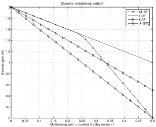
Figure 2: Diversity-multiplexing tradeoff of cooperative diversity schemes. There is one relay node between the source and its destination. Diversity gains $d_{M-AF,N=2}(r)$, $d_{DDF}(r)$ and $d_{NAF}(r)$ are obtained based on (134), (132) and (131) for $N=2$, respectively, and $d_{A-stc}(r)=2-4r$.

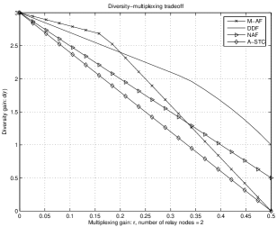
Figure 3: Diversity-multiplexing tradeoff of cooperative diversity schemes. There are two relay nodes between the source and its destination. Diversity gains $d_{M-AF,N=3}(r)$, $d_{DDF}(r)$ and $d_{NAF}(r)$ are obtained based on (135), (132) and (131) for $N=3$, respectively, and $d_{A-stc}(r)=3-6r$ is obtained in Section III-C.

III-D1 One-Relay Case

First suppose there is only one relay node between $N_{S}$ and $N_{D}$ and there are two phases in transmission as assumed in Section II. The proposed mixing strategy works as follows. Assume the channel fading parameter $\alpha_{S,R}$ can be measured perfectly at a relay node such that it can determine whether there will be an outage given current channel realizations. If there is no outage, the relay node works similarly as described in previous sections by performing decode-and-forward; otherwise, instead of dropping the received source packets, relay amplify-and-forwards the incoming source signals with an amplifying coefficient $\beta=\sqrt{\frac{P}{P|\alpha_{S,R}|^{2}+N_{0}}}$ to maintain its constant transmission power. It turns out the overall diversity-multiplexing tradeoff can be improved by this simple mixing scheme as shown next.

It has been proved in [8] that the AF and selection decode-and-forward schemes for a single relay network have the same DM-tradeoff function: $d_{AF}(r)=d_{DF}=2(1-2r)$, for $r\in[0,1/2]$. Applying the similar analytical approach as in Section III-A, the outage probability for a relay channel with only one relay node performing the decode-and-forward has an asymptotic equivalence consisting of two terms:

$$P_{out}\sim A\cdot\mbox{SNR}^{-(2-2r)}+B\cdot\mbox{SNR}^{-2(1-2r)},$$ (133)

where the first term is contributed by relay’s successful decoding and then independent encoding over successive two phases, the second term is due to relay’s dropping of the received signals because of its failure in decoding phase, $A$ and $B$ are some finite constants. Therefore, the overall DM-tradeoff is $d_{DF}(r)=2-4r$ due to the dominance of the slope $2-4r$ for $r\in[0,1/2]$.

Under the proposed mixing strategy, the slope in the first term of (133) is not affected when relay succeeds in decoding. The second term is, however, changed to $\mbox{SNR}^{-(1-2r)-(2-4r)}$, where $(1-2r)$ is the slope characterizing the vanishing rate of the probability of $|\mathcal{D}(s)|=1$ as derived in (12) in Section III-A, and $(2-4r)$ is the slope for the AF scheme. Therefore, the mixing scheme has an overall DM-tradeoff

$$d_{M-AF,K=1}(r)=\left\{\begin{array}[]{ll}2-2r,&0\leq r\leq 1/4\\ 3-6r,&1/4<r\leq 1/2\end{array}\right.$$ (134)

which is strictly greater than $d_{DF}(r)=2-4r$ for any $r\in(0,1/2)$, and thus shows the advantage of mixing the amplify-and-forward scheme with the decode-and-forward scheme.

When $K=1$, the DM-tradeoff of NAF is $d_{NAF}(r)=2-3r,\,0\leq r\leq 1/2$ from (131). It shows NAF is dominated by M-AF for $0\leq r\leq 1/3$. As for the DDF scheme, the diversity gain is $d_{DDF}(r)=2(1-r)\geq d_{M-AF}(r)$. The preceding comparison is illustrated by Figure 2.

III-D2 Two-Relay Case

In this section, we generalize the idea of mixing strategy to a two-relay case, where we show mixing approach can even outperforms the DDF scheme for some subset of multiplexing gain $r$. The result is stated in the following Theorem:

Theorem 11

The overall DM-tradeoff $d_{M-AF,K=2}(r)$ of a two-relay channel under our proposed mixing strategy is

$$d_{M-AF,K=2}(r)=\left\{\begin{array}[]{ll}3-2r,&0\leq r\leq\frac{1}{6}\\ 4-8r,&\frac{1}{6}\leq r\leq\frac{1}{2}.\end{array}\right.$$ (135)

Proof:

The proof relies on the mixing protocol which exploits the DM-tradeoff for asynchronous cooperative diversity schemes studied in Section III-B and Section III-C. The mechanism of the proposed protocol for this 2-relay node M-AF scheme is subject to the outcome of decoding at two relay nodes.

When both relay nodes fail in decoding i.e. $|\mathcal{D}(s)|=0$, only one of them employs AF and another one drops the received signals. In this case, the conditional outage probability has $P_{out||\mathcal{D}(s)|=0}\sim\mbox{SNR}^{-2(1-2r)-(2-4r)}$, where $2(1-2r)$ is the absolute slope of the probability of $\{|\mathcal{D}(s)|=0\}$ and $(2-4r)$ is the slope of the outage probability under AF.

If $|\mathcal{D}(s)|=1$, WLOG, suppose $N_{R_{2}}$ fails and $N_{R_{1}}$ succeeds in decoding. Thereafter, $N_{R_{1}}$ performs decode-and-forward employing a complex Gaussian codebook independent of the source codebook, while node 2 applies AF forwarding a scaled copy of the received signal. The outage probability given one node is in the decoding set has an asymptotic equivalence $P_{out||\mathcal{D}(s)|=1}(M-AF,K=2)\sim\mbox{SNR}^{-(1-2r)-l_{0}(r)}$, where $(1-2r)$ is the slope for the probability of $\{|\mathcal{D}(s)|=1\}$ and $l_{0}(r)$ represents the vanishing rate of the outage probability in an equivalent channel between $N_{S}$ and $N_{D}$ across two relay nodes. Next, we look into the bounds on $l_{0}(r)$ under different assumptions on the relative delay $\tau$ and show $3-6r\leq l_{0}(r)\leq 3-4r$.

If the relative delay $\tau$ between two relays is in the order of an integer number of symbol periods, since $N_{R_{2}}$ employs the same codewords as the source which is independent of what $N_{R_{1}}$ transmits, the slope $l_{0}(r)$ is expected to lie between that of the repetition coding based distributed delay diversity and independent coding based delay diversity schemes, which are $3-6r$ and $3-4r$, respectively, as derived in Section III-B. Therefore,we have $3-6r\leq l_{0}(r)\leq 3-4r$ in this case.

If $|\tau|/T_{s}$ is a non-integer and $s(t)$ satisfies the condition specified in Theorem 7, the relay-destination link is equivalent to a two-user parallel flat fading channel in terms of DM-tradeoff. Consequently, the mutual information of the entire link in this case has an asymptotic equivalence the same as $\frac{1}{2}\left[I_{AF}+\log\left(1+\rho_{0}|\alpha_{R_{2},D}|^{2}\right)\right]$, where $I_{AF}$ is the mutual information for an AF scheme taking the form of $\log\left[1+\rho_{0}(|\alpha_{1}|^{2}+|\alpha_{2}|^{2})\right]$ as shown in [8], where $\alpha_{1}$ and $\alpha_{2}$ are independent complex Gaussian random variables. Therefore, we obtain $l_{0}(r)=3-4r$, the asymptotic term characterizing the vanishing rate of the synchronous space-time-coded diversity scheme when two relay nodes are both in the decoding set, as determined by Lemma 3.

From the preceding analysis we obtain $3-6r\leq l_{0}(r)\leq 3-4r$, which leads us to

$$\mbox{SNR}^{-(4-8r)} \stackrel{{\scriptstyle<}}{{\sim}} P_{out||\mathcal{D}(s)|=1}(M-AF,N=3)$$ (136)

$$\stackrel{{\scriptstyle<}}{{\sim}} \mbox{SNR}^{-(4-6r)},\,r\in[0,1/2].$$

If two relay nodes both succeed in decoding i.e. $|\mathcal{D}(s)|=2$, the overall DM-tradeoff is equal to the asynchronous space-time-coded cooperative diversity approach yielding $P_{out||\mathcal{D}(s)|=2}\sim\mbox{SNR}^{-(3-2r)}$ under $\tau\in(0,T_{s})$ and $s(t)$ satisfying the condition in Theorem 7.

Putting all cases together, we can determine the overall DM-tradeoff averaged over all possible outcomes of the decoding set $\mathcal{D}(s)$, which is subject to the dominant term among $\{\mbox{SNR}^{-(4-8r)},\mbox{SNR}^{-(4-6r)},$ $\mbox{SNR}^{-(3-2r)}\}$ subject to $r$. For $r\in[0,1/6]$, $\mbox{SNR}^{-(3-2r)}$ is the slowest one, hence, $d_{M-AF,N=3}(r)=3-2r$; for $r\in(1/6,1/2]$, $\mbox{SNR}^{-(4-8r)}$ is the dominant one, we have $d_{M-AF,N=3}(r)=4-8r$. We thus complete the proof of Theorem 11.

∎

From this case study, we can conclude the mixing strategy does improve the DM-tradeoff over the pure decode-and-forward approach having $d_{A-stc}=3-6r$. Moreover, comparing (135) with (132) and (131) for $K=2$, we find the proposed mixing strategy outperforms DDF and NAF for $r\in[0,1/5]$, and $r\in[0,1/3]$, respectively, as shown in Figure 3. This observation demonstrates in order to improve the overall DM-tradeoff for cooperative diversity schemes in relay channels, we need to consider approaches which not only relax the restriction on sources transmitting only half of the total degrees of freedom as DDF and NAF in [16], but also exploit advantages of employing asynchronous coded schemes as demonstrated above using the proposed mixing strategy.

$|\mathcal{D}(s)|$	S-STC	ICB-DD	RCB-DD	ICB-DD-L	A-STC
$0$, $0\leq r\leq 1/2$	$3-6r$	$3-6r$	$3-6r$	$3-6r$	$3-6r$
$1$	$3-4r$	$3-4r$	$3-4r$	$3-4r$	$3-4r$
$2$	$3-4r$	$\in[3-6r,3-4r]$	$\in[3-6r/\Delta_{1},3-6r]$	$3-4r$	$3-2r$
Overall DM-tradeoff	$3-6r$	$3-6r$	$\in[3-6r/\Delta_{1},3-6r]$	$3-6r$	$3-6r$

TABLE I: Table of the vanishing rates of outage probabilities conditioned on the number of relay nodes available to forward, denoted by $|\mathcal{D}(s)|$. The multiplexing gain is denoted by $0\leq r\leq 1/2$. The acronyms are defined as: S-STC, Synchronous Space-Time Coded scheme (Section III-A); ICB-DD, Independent Coding Based Distributed Delay diversity (Section III-B1); RCB-DD, Repetition Coding Based Distributed Delay diversity (Section III-B2); ICB-DD-L, Independent Coding Based Distributed Delay diversity with Linearly modulated waveforms(Section III-B3); A-STC, Asynchronous Space-Time Coded scheme (Section III-C).

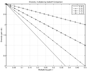
Figure 4: Numerical Comparison of DM-tradeoff functions listed in Table I for $0\leq r\leq 1/2$ and $\Delta_{1}=3/4$.

IV Conclusions

In this paper, we first show the lower-bound of the diversity-multiplexing tradeoff developed by [9] is actually the exact value for a synchronous space-time coded cooperative diversity scheme. We then propose two asynchronous cooperative diversity schemes, namely, independent coding based distributed delay diversity and asynchronous space-time coded relaying schemes. In terms of the overall DM-tradeoff, both of them achieve the same performance as the synchronous one, which demonstrates even at the presence of unavoidable asynchronism between relay nodes, we don’t loose diversity. Moreover, when all relay nodes succeed in decoding the source information, the asynchronous space-time coded approach achieves a better DM-tradeoff than the synchronous scheme does and performs equivalently to transmitting information through a parallel fading channel as far as the diversity order is concerned. Table I summarizes the results regarding the slope of conditional outage probability with respect to high SNR given $0\leq|\mathcal{D}(s)|\leq 2$ number of relay nodes available to forward. The acronyms are defined as: S-STC, Synchronous Space-Time Coded scheme (Section III-A); ICB-DD, Independent Coding Based Distributed Delay diversity (Section III-B1); RCB-DD, Repetition Coding Based Distributed Delay diversity (Section III-B2); ICB-DD-L, Independent Coding Based Distributed Delay diversity with Linearly modulated waveforms(Section III-B3); A-STC, Asynchronous Space-Time Coded scheme (Section III-C). Figure 4 provides a comparison of slope functions listed in Table I.

In analyzing the asymptotic performance of various approaches, a bottleneck on the overall DM-tradeoff in relay channels is identified. It is caused by restricting sources transmitting only in the first phase and relay nodes to employing decode-and-forward strategy. A simple mixing strategy is proposed to address this issue. By comparing it with the NAF and DDF proposed by [16], we show the mixing strategy achieves higher diversity gain than both DDF and NAF over certain range of the multiplexing gain $r$ even though we still let source transmit only half of an entire frame.

As observed in Section III-C, employing properly designed $s(t)$ of a finite duration $T_{s}$ can even lead to higher mutual information than synchronous space-time codes for any SNR. This reveals the advantage of fully exploiting both spatial and temporal degrees of freedom in MIMO systems by employing asynchronous space-time codes even in a frequency non-selective fading channel. The design of $s(t)$ and asynchronous space-time codes, as well as the corresponding performance analysis is beyond the scope of this paper and will be addressed in our future work.

Appendix A Appendix

A-A Proof of Lemma 1

Proof:

For each subset $A_{i}$ of $\tilde{\mathcal{A}}=\bigcup_{i=1}^{4}\tilde{\mathcal{A}}_{i}$ as defined in Section III-A, we calculate the corresponding integrals in (III-A) individually.

Over $\tilde{\mathcal{A}}_{1}=\left\{\beta_{S,D}\geq 1,\beta_{R_{1},D}\geq 1\right\}$, we have

$$\int_{\beta_{i,D}\in\tilde{\mathcal{A}_{1}}}\left(\log\widetilde{\mbox{SNR}}\right)^{2}\prod_{k\in\{S,R_{1}\}}\widetilde{\mbox{SNR}}^{-\beta_{k,D}}\tilde{\lambda}_{k,D}\,d\beta_{k,D}=$$

$$\prod_{k\in\{S,R_{1}\}}\tilde{\lambda}_{k,D}\left[\int_{1}^{\infty}\widetilde{\mbox{SNR}}^{-\alpha}\left(\log\widetilde{\mbox{SNR}}\right)\,d\alpha\right]^{2}$$

$$=\prod_{k\in\{S,R_{1}\}}\tilde{\lambda}_{k,D}\frac{1}{\widetilde{\mbox{SNR}}^{2}}.$$ (137)

Over $\tilde{\mathcal{A}}_{2}=\left\{\beta_{S,D}\geq 1,\right.$ $\left.1-2r<\beta_{R_{1},D}<1\right\}$ or $\tilde{\mathcal{A}}_{3}=\left\{1-2r<\beta_{S,D}<1,\beta_{R_{1},D}\geq 1\right\}$ the integral is

$$\int_{\beta_{i,D}\in\tilde{\mathcal{A}_{i}}}\left(\log\widetilde{\mbox{SNR}}\right)^{2}\prod_{k\in\{S,R_{1}\}}\widetilde{\mbox{SNR}}^{-\beta_{k,D}}\tilde{\lambda}_{k,D}\,d\beta_{k,D}=$$

$$\prod_{k\in\{S,R_{1}\}}\tilde{\lambda}_{k,D}\int_{1}^{\infty}\int_{1-2r}^{1}\widetilde{\mbox{SNR}}^{-(\alpha_{1}+\alpha_{2})}\cdot\left(\log\widetilde{\mbox{SNR}}\right)^{2}\,d\alpha_{2}\,d\alpha_{1}$$

$$=\prod_{k\in\{S,R_{1}\}}\tilde{\lambda}_{k,D}\frac{\left(\widetilde{\mbox{SNR}}\right)^{2r}-1}{\widetilde{\mbox{SNR}}^{2}},\,i=2,3.$$ (138)

Over $\tilde{\mathcal{A}}_{4}=\left\{0\leq\beta_{k,D}<1,\right.$ $\left.\sum_{k\in\{S,R_{1}\}}\right.$ $\left.\beta_{k}>2-2r\right\}$, we obtain

$$\int_{\beta_{i,D}\in\tilde{\mathcal{A}_{4}}}\left(\log\widetilde{\mbox{SNR}}\right)^{2}\prod_{k\in\{S,R_{1}\}}\widetilde{\mbox{SNR}}^{-\beta_{k,D}}\tilde{\lambda}_{k,D}\,d\beta_{k,D}=$$

$$\prod_{k\in\{S,R_{1}\}}\tilde{\lambda}_{k,D}\int_{1-2r}^{1}\int_{2-2r-\alpha_{1}}^{1}\widetilde{\mbox{SNR}}^{-(\alpha_{1}+\alpha_{2})}\cdot\left(\log\widetilde{\mbox{SNR}}\right)^{2}\,d\alpha_{2}\,d\alpha_{1}$$

$$=\prod_{k\in\{S,R_{1}\}}\tilde{\lambda}_{k,D}\left[\left(2r\log\widetilde{\mbox{SNR}}-1\right)\cdot\right.$$

$$\left.\left(\widetilde{\mbox{SNR}}\right)^{-(2-2r)}-\widetilde{\mbox{SNR}}^{-2}\right].$$ (139)

Combining (A-A)-(A-A), we obtain the RHS of (1)

$$\int_{\beta_{i,D}\in\tilde{\mathcal{A}}}\left(\log\widetilde{\mbox{SNR}}\right)^{2}\prod_{k\in\{S,R_{1}\}}\widetilde{\mbox{SNR}}^{-\beta_{k,D}}\tilde{\lambda}_{k,D}\,d\beta_{k,D}=$$

$$\prod_{k\in\{S,R_{1}\}}\tilde{\lambda}_{k,D}\left(1+2r\log\widetilde{\mbox{SNR}}\right)\left(\widetilde{\mbox{SNR}}\right)^{-(2-2r)}$$

$$\sim\left(2r\log\widetilde{\mbox{SNR}}\right)\left(\widetilde{\mbox{SNR}}\right)^{-(2-2r)}\prod_{k\in\{S,R_{1}\}}\tilde{\lambda}_{k,D},$$ (140)

which completes the proof of Lemma 1.

∎

A-B Proof of Lemma 3

Proof:

To derive the asymptotic equivalence of $\mbox{Pr}\left[I_{stc}<R,\;|{\mathcal{D}}(s)|=2\right]$, WLOG, assume $\tilde{\lambda}_{R_{1},D}>\tilde{\lambda}_{R_{2},D}$ and denote $y=\sum_{k\in{\mathcal{D}}(s)}|\tilde{\alpha}_{k,D}|^{2}$. The probability density function (pdf) of $y$ is

$$p(y)=\frac{\tilde{\lambda}_{R_{1},D}\tilde{\lambda}_{R_{2},D}}{\tilde{\lambda}_{R_{1},D}-\tilde{\lambda}_{R_{2},D}}\left(e^{-\tilde{\lambda}_{R_{2},D}y}-e^{-\tilde{\lambda}_{R_{1},D}y}\right),\;y\geq 0.$$

Define a normalized random variable $\beta_{R,D}=-\frac{\log y}{\log{\widetilde{\mbox{SNR}}}}$ whose pdf is

$$p(\beta_{R,D})=\frac{\tilde{\lambda}_{R_{1},D}\tilde{\lambda}_{R_{2},D}}{\tilde{\lambda}_{R_{1},D}-\tilde{\lambda}_{R_{2},D}}\exp\left\{-\lambda_{R_{2},D}\widetilde{\mbox{SNR}}^{-\beta_{R,D}}\right\}\cdot$$

$$\left[1-\exp\left\{-\left(\tilde{\lambda}_{R_{1},D}-\tilde{\lambda}_{R_{2},D}\right)\widetilde{\mbox{SNR}}^{-\beta_{R,D}}\right\}\right]\cdot\left(\log\widetilde{\mbox{SNR}}\right)\widetilde{\mbox{SNR}}^{-\beta_{R,D}}$$

$$\sim\tilde{\lambda}_{R_{1},D}\tilde{\lambda}_{R_{2},D}\left(\log\widetilde{\mbox{SNR}}\right)\widetilde{\mbox{SNR}}^{-2\beta_{R,D}},$$ (141)

for large $\widetilde{\mbox{SNR}}$ and $\beta_{R,D}\geq 0$. The conditional outage probability given two relay nodes are both in the decoding set ${\mathcal{D}}(s)$ is

$$\mbox{Pr}\left[I_{stc}<R||{\mathcal{D}}(s)|=2\right]\sim\int_{\beta_{i,D}\in\hat{\mathcal{A}}}\left(\log\widetilde{\mbox{SNR}}\right)^{2}$$

$$\widetilde{\mbox{SNR}}^{-\beta_{S,D}-2\beta_{R,D}}\prod_{k\in\left\{S,R_{1},R_{2}\right\}}\tilde{\lambda}_{k,D}\,d\beta_{S,D}d\beta_{R,D},$$ (142)

where

$$\hat{\mathcal{A}}=\left\{\underline{\beta}:{\sum_{i\in\left\{S,R\right\}}(1-\beta_{i,D})^{+}}<2r,\beta_{i,D}\geq 0\right\}.$$

By employing the same method as the one through which (1) is obtained, it can be shown that

$$\mbox{Pr}\left[I_{stc}<R||{\mathcal{D}}(s)|=2\right]\sim$$

$$2\prod_{k\in\left\{S,R_{1},R_{2}\right\}}\tilde{\lambda}_{k,D}\left(\widetilde{\mbox{SNR}}\right)^{-3+4r}\left[1-\frac{1}{2}\left(\widetilde{\mbox{SNR}}\right)^{-2r}\right]$$

$$\sim 2\prod_{k\in\left\{S,R_{1},R_{2}\right\}}\tilde{\lambda}_{k,D}\left(\widetilde{\mbox{SNR}}\right)^{-3+4r}.$$ (143)

As for the probability of $|\mathcal{D}(s)|=2$, we have $\mbox{Pr}\left[\left|{\mathcal{D}}(s)\right|=2\right]\sim 1$ resulting from (12). Thus, the overall conditional outage probability is

$$\mbox{Pr}\left[I_{stc}<R,\;|{\mathcal{D}}(s)|=2\right]\sim 2\prod_{k\in\left\{S,R_{1},R_{2}\right\}}\tilde{\lambda}_{k,D}\left(\widetilde{\mbox{SNR}}\right)^{-3+4r},$$

which completes the proof of Lemma 3.

∎

A-C Proof of Theorem 5

Proof:

Given $|\mathcal{D}(s)|=2$, the canonical receiver for the resulting equivalent $2$-path fading channel consists of a whitened matched filter (WMF) and a symbol rate sampler [47]. The Fourier transform of the impulse response of this equivalent channel is $F(f)=H(f)S(f)$, where $H(f)=\sum_{k}\alpha_{R_{k},D}e^{-j2\pi f\tau_{k}}$ and $S(f)$ is the Fourier transform of $s(t)$. The mutual information of this $2$-path fading channel given $\{\alpha_{R_{k},D}=r_{k}e^{j\theta_{k}}\}$ is [47, pp. 2597]

$$I_{2-TDA}=\frac{1}{2\pi}\int_{-\pi}^{\pi}\log\left[1+\rho_{0}|S_{hh}(\omega)|^{2}\right]\,d\omega,$$ (144)

where $|S_{hh}(\omega)|^{2}=\sum_{k}h(k)e^{jk\omega}$ is the discrete Fourier transform of $h(k)$, which is the sampling output of the matched filter for $F(t)=s(t)\alpha_{R_{1},D}+s(t-\tau)\alpha_{R_{2},D}$, i.e.

$$h(k)=\int_{-\infty}^{\infty}F(t)F^{*}(t-kT_{s})\,dt,$$

with $\tau=\tau_{2}-\tau_{1}$ denoted as the relative delay. WLOG, we assume $\tau\in(0,T_{s}]$ [42]. Due to the time-limited constraint on $s(t)$, we obtain $h_{k}=0$ for $|k|\geq 2$, and

$$h(0)=|\alpha_{R_{1},D}|^{2}+|\alpha_{R_{2},D}|^{2}+\rho_{12}\left(\alpha_{R_{1},D}\alpha_{R_{2},D}^{*}+\alpha_{R_{2},D}\alpha_{R_{1},D}^{*}\right)$$ (145)

and

$$h(1)=\alpha_{R_{2},D}\alpha_{R_{1},D}^{*}\rho_{21},\,h(-1)=\alpha_{R_{1},D}\alpha_{R_{2},D}^{*}\rho_{21},$$ (146)

where $\rho_{12}$ and $\rho_{21}$ are correlation coefficients of $s(t)$ determined by $\rho_{12}=\int_{0}^{T_{s}}s(t)s(t-\tau)\,dt$ and $\rho_{21}=\int_{0}^{T_{s}}s(t)s(t+T_{s}-\tau)\,dt$.

From Cauchy Schwartz inequality and $\int_{0}^{T_{s}}|s(t)|^{2}\,dt=1$, we have $|\rho_{12}|<1$ and $|\rho_{21}|\leq 1$ for $\tau\in(0,T_{s}]$, and

$$|\rho_{12}|+|\rho_{21}|=$$

$$\left|\int_{0}^{T_{s}}s(t)s(t-\tau)\,dt\right|+\left|\int_{0}^{T_{s}}s(t)s(t+T_{s}-\tau)\,dt\right|$$

$$\leq\int_{0}^{T_{s}}|s(t)|\left(|s(t-\tau)|+|s(t+T_{s}-\tau)|\right)\,dt\leq$$

$$\left[\int_{0}^{T_{s}}|s(t)|^{2}\,dt\right]^{1/2}\left[\int_{0}^{T_{s}}\left(\left|s(t-\tau)\right|+\left|s(t+T_{s}-\tau)\right|\right)^{2}\,dt\right]^{1/2}$$

$$=1.$$ (147)

Substituting $h(k)$ into $|S_{hh}(\omega)|^{2}$ yields

$$I_{2-TDA}=$$

$$\frac{1}{2\pi}\int_{-\pi}^{\pi}\log\left[1+\rho_{0}\left(|\alpha_{R_{1},D}|^{2}+|\alpha_{R_{2},D}|^{2}+\alpha_{R_{1},D}\alpha_{R_{2},D}^{*}\right.\right.$$

$$\left.\left.(\rho_{12}+\rho_{21}e^{j\omega})\alpha^{*}_{R_{1},D}\alpha_{R_{2},D}(\rho_{12}+\rho_{21}e^{-j\omega})\right)\right]\,d\omega$$

$$=\frac{1}{2\pi}\int_{-\pi}^{\pi}\log\left[1+\rho_{0}\left(\left|\alpha_{R_{1},D}+\alpha_{R_{2},D}(\rho_{12}+\rho_{21}e^{-j\omega})\right|^{2}\right.\right.$$

$$\left.\left.+|\alpha_{R_{2},D}|^{2}\left(1-\left|\rho_{12}+\rho_{21}e^{-j\omega}\right|^{2}\right)\right)\right]\,d\omega$$

$$=\frac{1}{2\pi}\int_{-\pi}^{\pi}\log\left[1+a+b\cos(\theta_{1}-\theta_{2}+\omega)\right]\,d\omega$$

$$=\log\left[1+a+\sqrt{(1+a)^{2}-b^{2}}\right]-1$$ (148)

where the last equality is from Eq. (32) with $a$ and $b$ defined as:

$$a = \rho_{0}\left(|r_{1}|^{2}+|r_{2}|^{2}+2\rho_{12}r_{1}r_{2}\cos(\theta_{1}-\theta_{2})\right)$$

$$= \rho_{0}\left(\left|\alpha_{R_{1},D}+\alpha_{R_{2},D}\rho_{12}\right|^{2}+|\alpha_{R_{2},D}|^{2}(1-|\rho_{12}|^{2})\right)$$

$$b = 2\rho_{21}r_{1}r_{2}\rho_{0}.$$ (149)

Given $|\rho_{12}|+|\rho_{21}|\leq 1$, it can be shown $a\geq b$ and $a\geq 0$ which enables us to bound $I_{2-TDA}$ in (A-C) by

$$I_{2-TDA}^{(L)}\stackrel{{\scriptstyle\bigtriangleup}}{{=}}\log\left[1+a\right]-1\leq I_{2-TDA}\leq I_{2-TDA}^{(U)}\stackrel{{\scriptstyle\bigtriangleup}}{{=}}\log\left[1+a\right].$$ (150)

Define random variables $X_{1}=\alpha_{R_{1},D}+\alpha_{R_{2},D}\rho_{12}$ and $X_{2}=\alpha_{R_{2},D}\sqrt{1-|\rho_{12}|^{2}}$. We can then rewrite $I_{2-TDA}^{(U)}=\log\left[1+\rho_{0}(|X_{1}|^{2}+|X_{2}|^{2})\right]$ and $I_{2-TDA}^{(L)}=\log\left[1+\rho_{0}(|X_{1}|^{2}+|X_{2}|^{2})\right]-1$. Clearly, the vector $[X_{1},X_{2}]^{\prime}$ is a linear transformation of the random vector $[\alpha_{R_{1},D},\alpha_{R_{2},D}]^{\prime}$, i.e.

$$\left[\begin{array}[]{l}X_{1}\\ X_{2}\end{array}\right] = \left[\begin{array}[]{ll}1&\rho_{12}\\ 0&\sqrt{1-|\rho_{12}|^{2}}\end{array}\right]\left[\begin{array}[]{l}\alpha_{R_{1},D}\\ \alpha_{R_{2},D}\end{array}\right]={\bf B}\left[\begin{array}[]{l}\alpha_{R_{1},D}\\ \alpha_{R_{2},D}\end{array}\right]$$ (159)

$$= {\bf B}\left[\begin{array}[]{ll}\sigma_{R_{1},D}&0\\ 0&\sigma_{R_{2},D}\end{array}\right]\left[\begin{array}[]{l}\hat{\alpha}_{R_{1},D}\\ \hat{\alpha}_{R_{2},D}\end{array}\right],$$ (164)

where

$$B=\left[\begin{array}[]{ll}1&\rho_{12}\\ 0&\sqrt{1-|\rho_{12}|^{2}}\end{array}\right],$$

and the entries of $\left[\hat{\alpha}_{R_{1},D},\hat{\alpha}_{R_{2},D}\right]^{{}^{\prime}}$ are i.i.d. complex Gaussian random variables with zero mean and unit variance. Define a upper-triangle matrix

$${\bf A}={\bf B}\left[\begin{array}[]{ll}\sigma_{R_{1},D}&0\\ 0&\sigma_{R_{2},D}\end{array}\right].$$

The matrix ${\bf A}$ can therefore be decomposed as ${\bf A}={\bf U}{\bf D_{A}}{\bf U}^{\dagger}$ using singular value decomposition, where ${\bf U}$ is a unitary matrix and ${\bf D_{A}}=\mbox{diag}\left[\sigma_{R_{1},D},\sigma_{R_{2},D}\cdot\sqrt{1-|\rho_{12}|^{2}}\right]$ is a diagonal matrix whose diagonal entries are the eigenvalues of the upper-triangular matrix ${\bf A}$. Decomposing ${\bf A}$ as such, we obtain $|X_{1}|^{2}+|X_{2}|^{2}=|\tilde{\alpha}_{R_{1}}|^{2}+|\tilde{\alpha}_{R_{2}}|^{2}\sqrt{1-|\rho_{12}|^{2}}$, where $[\tilde{\alpha}_{R_{1}},\tilde{\alpha}_{R_{2}}]^{\prime}$ is a vector having the same joint distribution as $[\alpha_{R_{1},D},\alpha_{R_{2},D}]$. Given the bounds on $I_{2-TDA}$, the overall mutual information $I_{L-TDA}$ can be bounded accordingly as $I_{L-TDA}\in[I_{L-TDA}^{(L)},I_{L-TDA}^{(U)}]$, where $I_{L-TDA}^{(L)}$ and $I_{L-TDA}^{(U)}$ are

$$I_{L-TDA}^{(L)}=\frac{1}{2}\log\left(1+\rho_{0}|\alpha_{S,D}|^{2}\right)+$$

$$\frac{1}{2}\log\left[1+\rho_{0}|\tilde{\alpha}_{R_{1}}|^{2}+\rho_{0}|\tilde{\alpha}_{R_{2}}|^{2}\sqrt{1-|\rho_{12}|^{2}}\right]-1$$ (165)

and

$$I_{L-TDA}^{(U)}=\frac{1}{2}\log\left(1+\rho_{0}|\alpha_{S,D}|^{2}\right)+$$

$$\frac{1}{2}\log\left[1+\rho_{0}|\tilde{\alpha}_{R_{1}}|^{2}+\rho_{0}|\tilde{\alpha}_{R_{2}}|^{2}\sqrt{1-|\rho_{12}|^{2}}\right].$$ (166)

As shown previously, given $\int_{0}^{T_{s}}|s(t)|^{2}\,dt=1$, for any $\tau\in(0,T_{s}]$, we have $|\rho_{12}|<1$ and thus $1-|\rho_{12}|^{2}>0$ which implies the asymptotic behavior of outage probabilities $\mbox{Pr}\left[I_{L-TDA}^{(U)}<R,|\mathcal{D}(s)|=2\right]$ and $\mbox{Pr}\left[I_{L-TDA}^{(L)}<R,|\mathcal{D}(s)|=2\right]$ is similar as the one characterized by Lemma 3 for synchronous space-time coded cooperative diversity scheme. Therefore, applying the same techniques in proving Lemma 3 yields (5) and thus Theorem 5 is proved.

∎

A-D Proof of Theorem 7

Proof:

Denote $\underline{S}(t)=[s(t),s(t-\tau)]^{T}$ and $\underline{S}_{w}(t)=\sum_{k=-2}^{2}\underline{S}(t-kT_{s})e^{jk\omega}$, where $s(t)=0,t\notin[0,2T_{s}]$. The matrix ${\bf\tilde{T}_{E}}(\omega)$ defined in (117) is :

$${\bf\tilde{T}_{E}}(\omega)=\sum_{k=-2}^{2}{\bf H_{E}}(k)e^{-jk\omega}=\int_{-\infty}^{\infty}\underline{S}(t)\underline{S}^{\dagger}_{w}(t)\,dt$$

$$=\int_{0}^{3T_{s}}\underline{S}(t)\underline{S}^{\dagger}(t)\,dt+e^{-j2\omega}\int_{0}^{T_{s}}\underline{S}(t)\underline{S}^{\dagger}(t+2T_{s})\,dt$$

$$+e^{j2\omega}\int_{2T_{s}}^{3T_{s}}\underline{S}(t)\underline{S}^{\dagger}(t-2T_{s})\,dt+e^{j\omega}\int_{T_{s}}^{3T_{s}}\underline{S}(t)\underline{S}^{\dagger}(t-T_{s})\,dt$$

$$+e^{-j\omega}\int_{0}^{2T_{s}}\underline{S}(t)\underline{S}^{\dagger}(t+T_{s})\,dt$$

$$=\int_{0}^{T_{s}}\left[\sum_{k=0}^{2}\underline{S}(t+kT_{s})e^{jk\omega}\right]\left[\sum_{k=0}^{2}\underline{S}(t+kT_{s})e^{jk\omega}\right]^{\dagger}\,dt,$$ (167)

where the above equations are derived by exploiting the finite duration of $s(t)$, as well as the definition of parameters in (74)-(77). As implied by the last equation in (A-D), ${\bf\tilde{T}_{E}}(\omega)$ is a non-negative definite matrix. This result can be extended in a similar manner to the case when $s(t)$ spans over any arbitrary finite $MT_{s}$ periods where $M\geq 1$ is an integer, i.e. $s(t)=0,t\notin[0,MT_{s}]$. Define $\underline{S}^{(M)}_{w}(t)=\sum_{k=-M}^{M}\underline{S}(t-kT_{s})e^{jk\omega}$. We obtain

$${\bf\tilde{T}_{E}}^{(M)}(\omega)=\int_{-\infty}^{\infty}\underline{S}(t)\left(\underline{S}^{(M)}_{w}(t)\right)^{\dagger}\,dt$$

$$=\int_{0}^{T_{s}}\left[\sum_{k=0}^{M}\underline{S}(t+kT_{s})e^{jk\omega}\right]\left[\sum_{k=0}^{M}\underline{S}(t+kT_{s})e^{jk\omega}\right]^{\dagger}\,dt,$$ (168)

which is a non-negative definite matrix for $M\geq 1$. Define $F_{1}(t,\omega)=\sum_{k=0}^{M}s(t+kT_{s})e^{jk\omega}$ and $F_{2}(t,\omega)=\sum_{k=0}^{M}s(t-\tau+kT_{s})e^{jk\omega}$ for all $t\in[0,T_{s}]$ and $\omega\in[-\pi,\pi]$. For a given $t$, $F_{1}(t,\omega)$ and $F_{2}(t,\omega)$ are the discrete time Fourier transforms of sampled signals of $s(t)$ and $s(t-\tau)$ at time instants $\left\{t+kT_{s},k=0,1,\cdots,M\right\}$, respectively. If there exists a non-zero complex vector $\underline{b}=[b_{0},b_{1}]$ such that $\underline{b}{\bf\tilde{T}_{E}}^{(M)}(\omega)\underline{b}^{\dagger}=0$ for some $\omega$, it indicates ${\bf\tilde{T}_{E}}^{(M)}(\omega)$ has a zero eigenvalue for the specified $\omega$, and thus we must have the following linear relationship associated with $F_{j}(t,\omega)$: $b_{0}F_{1}(t,\omega)+b_{1}F_{2}(t,\omega)=0$ for any $t\in[0,T_{s}]$. Therefore, if $s(t)$ is chosen to make $F_{1}(t,\omega)$ and $F_{2}(t,\omega)$ linearly independent with respect to $t$ for any given $\omega$, ${\bf\tilde{T}_{E}}^{(M)}(\omega)$ is always positive definite satisfying $\underline{b}{\bf\tilde{T}_{E}}^{(M)}(\omega)\underline{b}^{\dagger}>0$ for any non-zero $\underline{b}$ and $\forall\omega\in[-\pi,\pi]$. Let

$$G(\underline{b},\omega)=\underline{b}{\bf\tilde{T}_{E}}^{(M)}(\omega)\underline{b}^{\dagger}$$

$$=\int_{0}^{T_{s}}\left|b_{0}F_{1}(t,\omega)+b_{1}F_{2}(t,\omega)\right|^{2}\,dt,\,||\underline{b}||=1,$$ (169)

denote a continuous function of $\underline{b}$ and $\omega$ defined over a closed and bounded region, where $||\underline{b}||$ is the Euclidean norm of $\underline{b}$. Define

$$\lambda^{(M)}_{\mbox{min}}=\inf_{\omega\in[0,2\pi],||\underline{b}||=1}G(\underline{b},\omega),\,\lambda^{(M)}_{\mbox{max}}=\sup_{\omega\in[0,2\pi],||\underline{b}||=1}G(\underline{b},\omega)$$

By Weierstrass’ Theorem [48, pp. 654], the greatest lower bound $\lambda^{(M)}_{\mbox{min}}$ and least upper bound $\lambda^{(M)}_{\mbox{max}}$ of $G(\underline{b},\omega)$ is attainable. Therefore, if $s(t)$ is properly selected as specified above which results in positive definite matrices ${\bf\tilde{T}_{E}}^{(M)}(\omega)$, $\lambda^{(M)}_{\mbox{min}}$ and $\lambda^{(M)}_{\mbox{max}}$ are achievable and both of them are positive. In addition, $\lambda^{(M)}_{\mbox{max}}$ can be further upper-bounded by some finite constant as shown below:

$$\lambda^{(M)}_{\mbox{max}}(\omega)=\sup_{||\underline{b}||=1}\underline{b}{\bf\tilde{T}_{E}}^{(M)}(\omega)\underline{b}^{\dagger}$$

$$\leq\mbox{Tr}\left({\bf\tilde{T}_{E}}^{(M)}(\omega)\right)=2\sum_{k=-M}^{M}\int_{-\infty}^{\infty}s(t)s(t-kT_{s})e^{-jk\omega}\,dt$$

$$\leq 2\sum_{k=-M}^{M}\left|\int_{-\infty}^{\infty}s(t)s(t-kT_{s})\,dt\right|$$

$$\leq 2\sum_{k=-M}^{M}\left[\int_{-\infty}^{\infty}|s(t)|^{2}\,dt\right]^{1/2}\left[\int_{-\infty}^{\infty}|s(t-kT_{s})|^{2}\,dt\right]^{1/2}$$

$$=2(2M+1),\,\omega\in[0,2\pi],$$ (170)

where the first and second inequalities are due to the positive definiteness of ${\bf\tilde{T}_{E}}^{(M)}(\omega)$, and Cauchy-Schwartz inequality yields the third inequality. The last equality is because $s(t)$ has unit energy.

When $M=2$, this proves Theorem 7. When $M=1$, i.e. the waveform $s(t)$ is confined within one symbol interval, the condition stated in [44, pp. 4] is a special case of our result which reduces to the following condition for $M=1$: $s(t)$ and $s(t-\tau)+s(t-\tau+T_{s})e^{j\omega}$ are linearly independent with respect to $t\in[0,T_{s}]$ which is equivalent to $s(t)$ and $s(t+T_{s}-\tau)e^{j\omega}$, as well as $s(t)$ and $s(t-\tau)$ are linearly independent over $t\in[0,\tau]$ and $t\in(\tau,T_{s}]$, respectively. Also, we can observe from the second equality in (A-D) that $\mbox{Tr}\left({\bf\tilde{T}_{E}}^{(M)}(\omega)\right)=2\int_{0}^{T_{s}}|s(t)|^{2}\,dt=2$ in this case. This fact will be exploited when we compare the mutual information of a MISO channel using asynchronous space-time codes with that employing synchronous space-time codes.

Actually, the condition under which ${\bf\tilde{T}_{E}}^{(1)}(\omega)$ is positive definite can be further exposed by looking more closely at the parameters defined in (74)-(77) for $s(t)=0,\,t\notin[0,T_{s}]$. In this case, it is straightforward to show that $a_{1}=d_{1}=c_{2}=f_{1}=0$ for $\tau_{2}\geq\tau_{1}$. Therefore, the product of eigenvalues of the Hermitian matrix ${\bf\tilde{T}_{E}}^{(1)}(\omega)$ is

$$\left(1+2a_{1}\cos\omega\right)^{2}-\left|c_{1}e^{-j\omega}+c_{2}e^{-j2\omega}+c_{0}+f_{1}e^{j\omega}\right|^{2}$$

$$=1-\left|c_{0}+c_{1}e^{-j\omega}\right|^{2}\geq 0$$ (171)

where the inequality can be shown as follows. As defined in (74)-(77), $c_{0}$ and $c_{1}$ are correlation coefficients of $s(t)$ determined by $c_{0}=\int_{0}^{T_{s}}s(t)s(t-\tau)\,dt$ and $c_{1}=\int_{0}^{T_{s}}s(t)s(t+T_{s}-\tau)\,dt$. From Cauchy Schwartz inequality and $\int_{0}^{T_{s}}|s(t)|^{2}\,dt=1$,

$$|c_{0}+c_{1}e^{-j\omega}|=|c_{0}+c_{1}e^{j\omega}|$$

$$=\left|\int_{0}^{T_{s}}s(t)\left[s(t-\tau)+s(t+T_{s}-\tau)e^{j\omega}\right]\,dt\right|\leq$$

$$\left[\int_{0}^{T_{s}}|s(t)|^{2}\,dt\right]^{1/2}\left[\int_{0}^{T_{s}}\left|s(t-\tau)+s(t+T_{s}-\tau)e^{j\omega}\right|^{2}\right]^{1/2}$$

$$=1$$ (172)

where the last equality is because $s(t-\tau)$ and $s(t+T_{s}-\tau)$ have no overlap over $t\in[0,T_{s}]$, and the inequality becomes equality when $s(t)=C\left[s(t-\tau)+s(t+T_{s}-\tau)e^{j\omega}\right]$ where $|C|=1$ is a constant. This demonstrates only when $s(t)$ and $s(t-\tau)+s(t-\tau+T_{s})e^{j\omega}$ are linearly independent with respect to $t\in[0,T_{s}]$ for any $\omega\in[-\pi,\pi]$, can we have a strict inequality in (A-D) which agrees with the condition on $s(t)$ in Theorem 7 and thus verifies it from another perspective for $M=1$.

Note when the waveform $s(t)$ is a truncated version of a squared-root-raised-cosine waveform [49] spanning over $M$ symbol intervals such that $\int_{0}^{(M+|k|)T_{s}}s(t)s(t-kT_{s})\,dt\approx\delta_{k}$, where $\delta_{0}=1$ and $\delta_{k}=0$ for $k\neq 0$, the sum of eigenvalues of the matrix can be approximated as $\mbox{Tr}\left({\bf\tilde{T}_{E}}^{(M)}(\omega)\right)\approx 2$. Again, this property will be exploited when we compare the mutual information of two MIMO systems employing synchronous and asynchronous space-time codes, respectively.

∎

Acknowledgment

The author would like to thank anonymous reviewers for their valuable suggestions for improving the presentation of this paper.

Shuangqing Wei Shuangqing Wei graduated in Electrical Engineering from Tsinghua University with BE and MS in 1995 and 1998 and then obtained his Ph.D in EE from the University of Massachusetts, Amherst in 2003. He is currently an Assistant Professor in the Department of Electrical and Computer Engineering at Louisiana State University. His areas of interest are in communication theory, information theory, coding theory and their applications to wireless networks.

References

• [1] E. C. can der Meulen, “Three-terminal communication channels,” Adv. Appl. Prob., vol. 3, pp. 120–154, 1971.
• [2] T. M. Cover and A. A. El Gamal, “Capacity theorems for the relay channel,” IEEE Trans. Inform. Theory, vol. 25, pp. 572–584, Sept. 1979.
• [3] G. Kramer, M. Gastpar, and P. Gupta, “Cooperative strategies and capacity theorems for relay networks,” IEEE Trans. Inform. Theory, vol. 51, no. 9, pp. 3037– 3063, Sept. 2005, submitted.
• [4] L.-L. Xie and P. Kumar, “A network information theory for wireless communication: scaling laws and optimal operation,” IEEE Trans. Inform. Theory, vol. 50, pp. 748–767, May 2004.
• [5] P. Gupta and P. Kumar, “Towards an information theory of large networks: an achievable rate region,” IEEE Trans. Inform. Theory, vol. 49, no. 8, pp. 1877– 1894, Aug. 2003.
• [6] A. Sendonaris, E. Erkip, and B. Aazhang, “User cooperation diversity-Part I: system description,” IEEE Trans. Commun, vol. 51, pp. 1927–1938, Nov. 2003.
• [7] ——, “User cooperation diversity - Part II: implementation aspects and performance analysis,” IEEE Trans. Commun, vol. 51, pp. 1939–1948, Nov. 2003.
• [8] J. N. Laneman, D. Tse, and G. Wornel, “Cooperative diversity in wireless networks: efficient protocols and outage behavior,” IEEE Trans. Inform. Theory, vol. 50, pp. 3062–3080, Dec. 2004.
• [9] J. N. Laneman and G. Wornell, “Distributed space-time coded protocols for exploiting cooperative diversity in wireless networks,” IEEE Trans. Inform. Theory, vol. 49, pp. 2415–2425, Oct. 2003.
• [10] J. Boyer, D. Falconer, and H. Yanikomeroglu, “Multihop diversity in wireless relaying channels,” IEEE Transactions on Communications, vol. 52, pp. 1820–1830, Oct 2004.
• [11] A. Stefanov and E. Erkip, “Cooperative coding for wireless networks,” in Proc. IEEE Conference on Mobile and Wireless Communications Networks, Stockholm, Sweden, Sept. 2002.
• [12] R. U. Nabar, H. Bölcskei, and F. W. Kneubühler, “Fading relay channels: Performance limits and space-time signal design,” IEEE Journal on Selected Areas in Communications, vol. 22, pp. 1099–1109, August 2004.
• [13] T. Hunter and A. Nosratinia, “Coded cooperation under slow fading, fast fading, and power control,” in Proc. Asilomar Conference on Signals, Systems, and Computers, Nov. 2002.
• [14] M. Janani, A. Hedayat, T. Hunter, and A. Nosratinia, “Coded cooperation in wireless communications: space-time transmission and iterative decoding,” IEEE Trans. Signal Proc., vol. 52, pp. 362–371, Feb. 2004.
• [15] M. A. Khojastepour, A. Sabharwal, and B. Aazhang, “On the capacity of ‘cheap’ relay networks,” in Proc. Conference on Information Sciences and Systems (CISS), March 2003.
• [16] K. Azarian, H. E. Gamal, and P. Schniter, “On the achievable diversity-multiplexing tradeoff in half-duplex cooperative channels,” IEEE Trans. Inform. Theory, vol. 51, no. 12, pp. 4152–4172, Dec. 2005.
• [17] R. Pabst, B. Walke, D. Schultz, P. Herhold, H. Yanikomeroglu, H. Mukherjee, S.and Viswanathan, M. Lott, W. Zirwas, H. Dohler, M.and Aghvami, D. Falconer, and G. Fettweis, “Relay-based deployment concepts for wireless and mobile broadband radio,” IEEE Communications Magazine, vol. 42, pp. 80–89, Sept. 2004.
• [18] B. E. Schein and R. Gallager, “The Gaussian parallel relay network,” in Proc. IEEE Int. Symp. Inform. Theory, June 2000, p. 22.
• [19] A. Host-Madsen and J. Zhang, “Capacity bounds and power allocation for wireless relay channels,” IEEE Trans. Inform. Theory, vol. 51, no. 6, pp. 2020–2040, June 2005.
• [20] S. M. Alamouti, “A simple transmit diversity technique for wireless communications,” IEEE J. Select. Areas Commun., vol. 16, pp. 1451–1457, Oct. 1998.
• [21] X. Li, “Energy efficient wireless sensor networks with transmission diversity,” Electronics Letters, vol. 39, no. 24, pp. 1753–1755, Nov. 27 2003.
• [22] D. Goeckel and Y. Hao, “Macroscopic space-time coding: motivation, performance criteria, and a class of orthogonal designs,” in Proc. Conference on Information Sciences and Systems (CISS), March 2003.
• [23] ——, “Space-time coding for distributed antenna arrays,” in IEEE International Conference on Communications (ICC), vol. 2, June 2004, pp. 747– 751.
• [24] S. Wei, D. Goeckel, and M. Valenti, “Asynchronous cooperative diversity,” in Proc. Conference on Information Sciences and Systems (CISS), Princeton, March 2004.
• [25] ——, “Asynchronous cooperative diversity,” IEEE Trans. on Wireless Communications, vol. 5, no. 6, pp. 1547– 1557, June 2006.
• [26] A. Scaglione and Y. W. Hong, “Opportunistic large arrays: cooperative transmission in wireless multihop ad hoc networks to reach far distances,” IEEE Trans. Signal Proc., vol. 51, pp. 2082–2092, Aug. 2003.
• [27] A. Dana and B. Hassibi, “On the power-efficiency of sensory and ad-hoc wireless networks,” IEEE Transactions on Information Theory, 2005.
• [28] R. U. Nabar and H. Bölcskei, “Capacity scaling laws in asynchronous relay networks,” in Proc. Allerton Conf. Commun., Control, Computing, Oct. 2004.
• [29] S. Wei, “Diversity-multiplexing tradeoff of asynchronous space-time-coded cooperative diversity,” Proc. Allerton Conf. Commun., Control, Computing, Oct. 2004.
• [30] ——, “How much asynchronism matters for exploiting cooperative diversity in ad hoc wireless networks,” in Proc. International Conference on Computing, Communications and Control Technologies: CCCT’04, Austin, TX, Aug. 2004.
• [31] L. Zheng and D. Tse, “Diversity and multiplexing: a fundamental tradeoff in multiple-antenna channels,” IEEE Transactions on Information Theory, vol. 49, no. 1073- 1096, May 2003.
• [32] D. Tse, P. Viswanath, and L. Zheng, “Diversity-multiplexing tradeoff in multiple-access channels,” IEEE Trans. Inform. Theory, vol. 50, pp. 1859– 1874, Sept. 2004.
• [33] T. S. Rappaport, Wireless Communications: Principles and Practice.   New Jersey: Prentice Hall, Inc., 1996.
• [34] G. Caire and S. Shamai, “On the achievable throughput of a multiantenna Gaussian broadcast channel,” IEEE Trans. Inform. Theory, vol. 49, no. 7, July 2003.
• [35] M. Costa, “Writing on dirty paper,” IEEE Trans. Inform. Theory, vol. 29, pp. 439–441, May 1983.
• [36] S. Wei and R. Kannan, “Strategic versus collaborative power control in relay fading channels,” in IEEE International Symposium on Information Theory (ISIT), Seattle, July 2006.
• [37] K. W. Breitung, Asymptotic Approximations for Probability Integrals, ser. Lecture Notes in Mathematics.   Springer-Verlag, 1994, no. 1592.
• [38] N. Seshadri and J. H. Winters, “Two signaling schemes for improving the error performance of frequency-division-duplex (FDD) transmission systems using transmitter antenna diversity,” in Proc. 43rd IEEE Vehicular Technology Conference, 1993, pp. 508–511.
• [39] R. G. Gallager, Information Theory and Reliable Communication.   New York: Wiley, 1968.
• [40] L. Ozarow, S. Shamai, and A. D. Wyner, “Information theoretic considerations for cellular mobile radio,” IEEE Trans. Veh. Technol., vol. 43, pp. 359–377, May 1994.
• [41] I. S. Gradshteyn and I. M. Ryzhik, Tables of Integrals, Series and Products, 6th ed.   New York: Academic Press, 1980.
• [42] R. Cheng and S. Verdu, “Capacity of root-mean-square bandlimited Gaussian multiuser channels,” IEEE Trans. Inform. Theory, vol. 37, pp. 453–465, May 1991.
• [43] S. Verdu, “The capacity region of the symbol-asynchronous Gaussian multiple-access channel,” IEEE Trans. Inform. Theory, vol. 35, pp. 733–751, July 1989.
• [44] R. Cheng and S. Verdu, “The effect of asynchronism on the total capacity of Gaussian multiple-access channels,” IEEE Trans. Inform. Theory, vol. 38, pp. 2–13, Jan. 1992.
• [45] S. Verdu, “Multiple-access channels with memory with and without frame synchronism,” IEEE Trans. Inform. Theory, vol. 35, pp. 605–619, May 1989.
• [46] H. Gazzah, P. A. Regalia, and J. P. Delmas, “Asymptotic eigenvalue distribution of block Toeplitz matrices and application to blind simo channel identification,” IEEE Trans. Inform. Theory, vol. 47, pp. 1243–1251, March 2001.
• [47] J. M. Cioffi, G. P. Dudevoir, M. V. Eyuboglu, and G. D. Forney, “MMSE decision-feedback equalizers and coding II: coding results,” IEEE Transactions on Communications, vol. 43, pp. 2595–2603, Oct. 1995.
• [48] D. P. Bertsekas, Nonlinear Programming, 2nd ed.   Athena Scientific, 1999.
• [49] J. G. Proakis, Digital Communications, 3rd ed.   New York: McGraw-Hill, 1995.