A Map-Based Model of the Cardiac Action Potential

Abstract

A discrete time model that is capable of replicating the basic features of cardiac cell action potentials is suggested. The paper shows how the map-based approaches can be used to design highly efficient computational models (algorithms) that enable large-scale simulations and analysis of discrete network models of cardiac activity.

I Introduction

The heart cells that are directly involved in the dynamics of its electrical activity include pacemaker and non-pacemaker cells. The peacemaker cells generate spontaneous action potentials and are characterized by a slow rate of the depolarization. These cells are found in sinoatrial and atrioventricular nodes of the heart and initiate the propagation of electrical activity throughout the heart. The non-pacemaker cells, involved in the propagation of electrical activity, such as atrial myocytes, ventricular myocytes and Purkinje cells, have a specific form of action potential (AP) which is characterized by five main phases including a very rapid depolarization and a prolonged plateau Eick81 , see Fig 1. This paper proposes a simple computationally efficient model that can replicate these phases of AP.

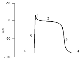
Figure 1: A sketch of typical action potential of a ventricular cell illustrates the main phases associated with different states of channel activity.

The non-pacemaker cell has a very negative resting potential (phase 4) characterized by the open potassium channels and, therefore, K⁺ current and the closed fast sodium Na⁺ and slow calcium channels Ca²⁺. Being depolarized to the threshold voltage of about -70mV the cell shows a very rapid depolarization caused by opening fast sodium channels Na⁺ (phase 0). This phase quickly increases the membrane potential to positive values where the Na⁺ channels become inactivated and the dynamics of the membrane changes to an initial repolarization (phase 1) induced by a short-term transient outward K⁺ current. The plateau of cardiac action potential (phase 2) is the result of balanced dynamics between inward Ca²⁺ current and the outward K⁺ current coming through the slow delayed rectifier potassium channels. A number of other ionic currents are also involved in this phase. As the Ca²⁺ channels start to close while the rectifier K⁺ channels remain open, the membrane potential drops to the levels of resting potential forming phase 3. Even from this, an overly simplified scenario involved in the formation cardiac action potential, it becomes clear that any attempt to produce a conductance based model of a non-pacemaker cell will lead to a large system of differential equations. A number of such models have been proposed and are used as accurate models of cardiac cells, see for example LuoRudy94a ; LuoRudy94b ; NobleRudy01

The simplified approaches to the modeling of cardiac ventricular action potentials include the sets of ODE models where each ODE equation phenomenologically represents the dynamics of multiple channels (for example, van der Pol equation vanderPoll28 or the FitzHugh-Negumo model FitzHugh61 ; Rogers94 ). However, due to the high depolarizing rates of AP during phase 0 numerical simulations with the ODE models require a significant reduction of the integration step size which complicates the use of these simple models in studies of large scale networks. Here we suggest a model of the cardiac AP which is built using a discrete time map and designed to significantly increase the time step of simulations. A similar approach was successfully used before in the design of computationally efficient models of spiking-bursting Rulkov02 , regular spiking and fast and spiking neurons RTB_CN04 , and other neurons.

II Map-based model of cardiac AP

The simplest form of the suggested model is a two-dimensional map, which can be written as

$$x_{n+1} = P(x_{n},y_{n})~{},$$ (1a)

$$y_{n+1} = Q(x_{n},y_{n})~{},$$ (1b)

where the dynamics of $x_{n}$ represents the fast changes related the phase 0 and the dynamics of $y_{n}$ forms the action potential during the remaining phases. The voltage of action potential $V_{n}$ will be defined at the end of this section as a liner combination of $x_{n}$ and $y_{n}$.

The function $P(x_{n},y_{n})$ in the right hand side of the first equation (1a) can be written as

$$P(x_{n},y_{n})=(1-\varepsilon(y_{n}))f(x_{n},x_{n-1},u)+\varepsilon(y_{n})x_{p},$$ (2)

where the nonlinear function $f(x_{n},x_{n-1},u)$ is of the form Rulkov02

$$f(x_{n},x_{n-1},u)=$$ (3)

$$\cases{\alpha/(1-x_{n})+u,&if $x_{n}\leq 0$\cr\alpha+u,&if $0<x_{n}<\alpha+u$ and $x_{n-1}\leq 0$\cr-1,&if $x_{n}\geq\alpha+u$ or $x_{n-1}>0.$\cr}$$

Note, that for a description of autonomous dynamics of the model the conditions related to the values of $x_{n-1}$ can be omitted. The third argument $u$ will represent a linear combination of the function parameter $\beta_{x}$ and the input variable (e.g. injected current)

$$u=\beta_{x}+I_{n}.$$ (4)

Parameter $\alpha$ is a control parameter of the map. The dependence of $f(x,u)$ on $x$ computed for fixed values of $u$ and $\varepsilon(y_{n})=0$, i.e. when $P(x_{n},y_{n})=f(x,u)$, is shown in Fig.2. This figure also illustrates a trajectory of an uncoupled one-dimensional map (1a). The limit cycle of the map was used in Rulkov02 to replicate a sequence of short neuronal action potentials - a spike train. Note, that the third condition of $f(x,u)$ corresponds to the moment of time when $x_{n}$ reaches its maximum value, i.e. the tip of a spike.

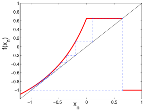
Figure 2: (Color online) The shape of $f(x_{n},u)$ and a limit cycle generated by subsystem (1a) with $\varepsilon(y_{n})=0$ and a fixed value of $u$=-2.55

To replicate the action potential of a cardiac ventricular cell we shift $f(x,u)$ down where the nonlinear segment intersects the diagonal giving birth to stable and unstable fixed points. This shift destroys the limit cycle shown in Fig.2. In addition to that we modulate the 1-D map with $\varepsilon(y_{n})$, where $0\leq\varepsilon(y_{n})\leq 1$, see (2). One can see from (2) that when $\varepsilon(y_{n})$ approaches one the $x$ dependance of function $P(x_{n},y_{n})$ flattens and approaches the values $P(x_{n},y_{n})\rightarrow x_{p}$ for all $x_{n}$. Therefore, the increase of $\varepsilon(y_{n})$ ”deactivates” the motions of the 1-D map (1a) by forming a superstable fixed point $x_{p}$. We will utilize this effect to replicate the blocking of Na⁺ channels to terminate phase 0, see Fig 1.

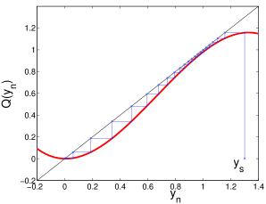
Figure 3: (Color online) The dependance of $Q(x_{n},y_{n})$ on $y_{n}$ and the trajectory of subsystem (1b) started at $y_{s}$=1.3 plotted for the parameter values $\mu=0.02$ and $g=1.0$.

When equation (1a) produces a spike the membrane potential rises and the other ionic channels get involved the formation of the plateau described above as phases 1,2 and 3. The dynamics of the cell during this part of AP is governed by subsystem (1b), where the right hand side can be written in the form

$$Q(x_{n},y_{n})= \cases{y_{s},&if $x_{n}\geq\alpha+u$ or $x_{n-1}>0,$\cr q(y_{n}),&otherwise.\cr}\$$ (5)

where

$$q(y_{n})=(1-\mu)y_{n}-gy_{n}(1-y_{n})^{2}.$$

Note that the first condition of (5) is the same as the third condition of (3) and corresponds to the moment of spike in subsystem (1a). One can see that at the moment of spike the trajectory of the subsystem (1b) starts at the value $y_{n}=y_{s}$ and then follows the dynamics of the one-dimensional map which is modeled here with a polynomial function $q(y_{n})$. Function $q(y_{n})$ is designed to form a stable fixed point at $y_{n}$=0 and a very narrow gap between the function and the diagonal where the trajectories of subsystem (1b) slow down, see Fig. 3. This slow motion is used to form the plateau in the shape of cardiac action potential, i.e. phase 2. The size of the gap and, therefore, the duration of the plateau, is set by selecting parameter $\mu$. The other control parameter $g$ of the function is used to shape the action potential at the transient from plateau to the resting state, i.e. phase 3. The idea behind the selection of these parameter values is illustrated in Fig 4. The duration and shape of the action potential can also be controlled by the location of starting point in equation (1b), i.e. parameter $y_{s}$.

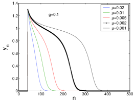
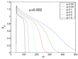
Figure 4: (Color online) Waveforms generated by subsystem (1b) with $y_{s}$=1.3 and different values of parameters $\mu$ (top panel) and $g$ (bottom panel).

In order to model the absolute refractory period (ARP) that prohibits triggering a new action potential during phases 1, 2 and the beginning part of phase 3 we deactivate subsystem (1a) using function $\varepsilon(y_{n})$ which can be defined as a step function

$$\varepsilon(y_{n})= \cases{0,&if $y_{n}\leq y_{th}$\cr 1,&if $y_{n}>y_{th}$.\cr}$$ (6)

Here, the value of $y_{th}$ sets the threshold of deactivation.

Equation (6) closes the feedback between subsystems (1a) and (1b), and completes the basic part of the map-based model. The membrane potential replicated by this model can be defined as

$$V[mV]=-25mV+x_{n}\times 80mV+y_{n}\times 85mV.$$ (7)

Examples of APs produced by this model are presented in Fig.5. The parameters $\alpha$ and $\beta_{x}$ of function (3), (4) are set to provide a stable fixed point in the subsystem (1a) at the negative values of $x_{n}$. This takes place when the nonlinear part of $f(x_{n})$ crosses the diagonal. The AP was triggered by a pulse of external current $I_{n}$, see (4). This pulse moves function $f(x_{n},u)$ up and, if the amplitude of the pulse is sufficient, the stable fixed point disappears via a saddle-node bifurcation in (1a). After that the trajectory $x_{n}$ goes up forming a short spike in the waveform of $x_{n}$. The time interval between the trigger pulse and the spike depends on the amplitude and duration of the pulse, see Fig. 5. The spike initiates the motion in subsystem (1b) by changing its state to $y_{n}=y_{s}$, see (5). After $y_{n}$ has occurred at the high level it deactivates subsystem (1a) by setting $\varepsilon(y_{n})=1$ and keeps it deactivated until $y_{n}$ gets to the levels below $y_{th}$, see (6).

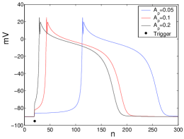
Figure 5: (Color online) Example of ventricular action potentials computed with formula (7). The parameter values are $\alpha=3.2$, $\beta_{x}=-2.5780$, $x_{p}=-0.8$, $y_{s}=1.3$, $\mu=0.002$, $g=0.2$, $y_{th}=0.5$ and three amplitudes $A_{p}$ of triggering pulses of external current $I_{n}$ which is applied at $n=20$ for one iteration.

Despite the simplicity of dynamical mechanisms included in the map-based model constructed above the model is capable of replicating a number of interesting properties of the behavior of ventricular cells. For example it can capture the effects of the coexistence of different oscillation regimes triggered by a periodic sequence of pulses. With proper selection of frequency and amplitude of the pulses the model can produce APs with the frequency ratio 1:2 or 1:1. These regimes are shown in Fig. 6. When in addition to the periodic sequence of pulses we add one more pulse unrelated to the periodic sequence the result depends on the phase of AP where the new pulse occurs. If the additional pulse falls within the absolute refractory period it does not affect the oscillations, see Fig. 6a. If the pulse occurs before or after the ARP it can switch the oscillations to the regime with a different frequency locking ratio, as it is shown in Fig. 6b. The coexistence of these regimes indicate the presence of a memory effect in the dynamics of cardiac AP. In this basic model the memory is the result of a transient in subsystem (1a) from the state $x_{p}$ to the fixed point after it has been activated. Similar phenomena caused by a memory effect have been studied in  Hall99 ; Tolkacheva02 ; Schaefer07 with a different type of mapping model.

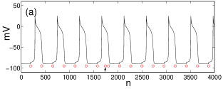
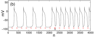
Figure 6: (Color online) Action potentials triggered by a periodic sequence of pulses (red circles) and one additional pulse indicated by the arrow. The amplitude of pulses $A=0.05$. The other parameters the same in Fig. 5. (a) Regime of oscillations with frequency ratio 1:2. (b) Transition from 1:2 to 1:1 frequency ratio caused by the additional pulse.

III Modeling of memory effects

Regulation and rate dependance of action potential duration (APD) is an important property of the ventricular cells LuoRudy94b ; HundRudy04 ; Franz03 . In the considered map-based model the effects related to APD adaptation can be achieved by modulation of the subsystem (1b) by dynamically varying the values of parameters $\mu$, $g$ or $y_{s}$, see (5). As an example consider the case when the parameter $y_{s}$ in (5) is substituted with a new variable $y_{s}^{new}=y_{s}-s_{n}$ and $s_{n}$ is described by equation of the form

$$s_{n+1}=\cases{S_{s},&if $x_{n}\geq\alpha+u$ or $x_{n-1}>0,$\cr q_{s}(s_{n}),&otherwise.\cr}\$$ (8)

where $q_{s}(s_{n})=s_{n}-g_{s}s_{n}(S_{a}-s_{n})$. This equation works similar to subsystem (1b),(5). When subsystem (1a) generate a spike the trajectory of (8) starts at $S_{s}$, ($0\leq S_{s}<S_{a}$) and drifts to $s_{n}=0$ with the rate controlled by parameter $g_{s}$, ($0<g_{s}<S_{a}^{-1}$). By selecting parameter values $S_{a}=0.6$, $S_{s}=0.599$, $g_{s}=0.02$ one can tune the evolution of $s_{n}$ to replicate the properties of the electrical restitution curves. An example of such an adaptive behavior is shown in Fig. 7. The figure presents a set of waveforms of two consecutive action potentials. The first AP is triggered at n=200 while the time of the second AP is varied by changing the timing of the second trigger pulse. One can see that due to dynamical modulation of $y_{s}$ the duration of the second AP is significantly reduced at the short time intervals between the trigger pulses. The APD recovers as the time interval increases. The shape of the restitution curve can be controlled by the parameters of system (8).

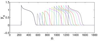
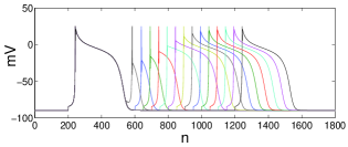
Figure 7: (Color online) Waveforms of $y_{n}$ and AP illustrating the effect of electrical restitution modeled by means of $y_{s}$ modulation using Eq. 8 with parameter values $S_{a}=0.6$, $S_{s}=0.599$, $g_{s}=0.02$. The parameter values of the map-models are the same as in Fig. 5 except for $A=0.69$, $g=0.1$ and $\mu=0.001$.

IV Modeling of electric coupling

An important component in the simulations of electrical activity of heart tissue is the model for electrical coupling among the cells. This coupling occurs through a gap junction between the nearby cells. A number for models describing the gap junction dynamics at different levels of sophistication have been suggested and reported Joyner86 ; Jamaleddine96 ; Henriquez01 . Here we will consider how the simplest gap junction model can be used to couple the cells in the form of map-based models. We assume that current flowing through the gap junction from cell $j$ into cell $i$ is

$$I_{n,j,i}^{gap}=g_{gap}(V_{n,j}-V_{n,i})$$ (9)

where $V_{n,i}$ is a membrane potential of cell $i$ given by Eq. (7) and $g_{gap}$ is the conductance of the gap junction, i.e. coupling strength parameter.

We will assume that at different phases of AP the current has different effects on the dynamics of the cell. For example, at the phases 0 and 4 the effect of coupling is more pronounced than during the phases 1,2 and 3. Therefore, to insert the gap junction current into the map-based model at the phases 0 and 4 we rewrite equation (4) by adding $I_{n,j,i}^{gap}$, i.e.

$$u=\beta_{x}+I_{n}+\sum_{j\in J}(I_{n,j,i}^{gap}),$$ (10)

where $J$ is the set of nearby cells. In order to capture the effect of the gap junction during the phases 1,2 and 3, when subsystem (1a) is turned off, one can rewrite equation (1b) as follows

$$y_{n+1} = Q(x_{n},y_{n})+\mu_{gap}\sum_{j\in J}(I_{n,j,i}^{gap})~{},$$ (11)

where parameter $\mu_{gap}$ can be selected to set a proper balance between the coupling strengths at different phases of AP.

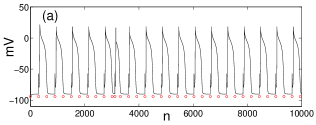
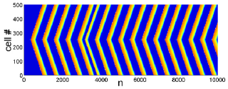
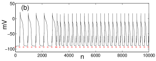
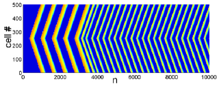
Figure 8: (Color online) Waveforms of $V_{n,250}$ triggered by the stimuli (red circles) and images of waves in the circle of 500 electrically coupled cells. Regime of frequency ratio 1:2 - (a) and a change to the regime of 1:1 caused by the proper position of the additional trigger pulse - (b)

To illustrate some of the effects captured by such a coupling model we consider a one-dimensional chain with periodic boundary conditions which contains 500 cells coupled to nearest neighbors. Electrical activity of this circle of cells was initiated by excitation of a single cell (cell number 250) using a periodic sequence of triggering pulses and one additional pulse, whose position in time was controlled independently of the periodic sequence. The amplitude of the trigger pulses was set $A=0.4$ and the duration of each pulse was one iteration long. The parameters of the cell model were selected as $\alpha=3.2$, $\beta_{x}=-2.5780$, $x_{p}=-0.8$, $y_{s}=1.3$, $\mu=0.001$, $g=0.1$, $y_{th}=0.01$, $S_{s}=0.399$, $S_{a}=0.4$ and $g_{s}=0.03$. The parameters of the gap junction model were set equal to $g_{gap}=0.004$ and $\mu_{gap}=0.0001$. The results of simulations are shown is Figs. 8 and 9.

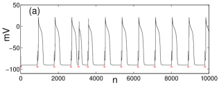
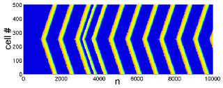
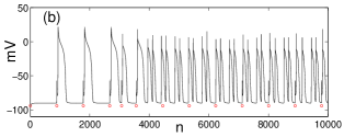
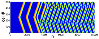
Figure 9: (Color online) Waveforms of $V_{n,250}$ triggered by the stimuli (red circles) and images of waves in the circle of 500 electrically coupled cells, without (a) and with (b) a group of ”damaged” cells.

Figure  8 illustrates the case of the coexistence of two regimes of wave activity with the frequency ratios 1:2 and 1:1. In Fig. 8(a) the additional trigger pulse has a phase that inserts perturbations into the wave behavior, but does not change the regime of activity after the transient is terminated. When the position of the additional pulse was moved closer to the end of the previous AP it was sufficient to switch the regime of activity from 1:2 to 1:1 frequency ratio. This effect is similar to the one shown in Fig. 6, but here the memory effects were controlled directly with (8). The sudden change of frequency ratio of the waves is typical for cases of high frequency triggering pulses and was demonstrated before in simulations with more realistic conductance-based models, see for example Stamp02 ; Kanakov07 .

Figure  9 shows the effect that can be caused by existence of a small group of ”damaged” cells on the wave activity of the chain. In this case the period between the triggering impulses is larger than the APD of normal cells and, when the parameters of all cells are the same, the APs with 1:1 frequency ratio is the only stable regime of wave activity in the chain. It is illustrated in Fig. 9(a) where the periodic waves perturbed by the additional trigger pulse recover very fast. The situation with the recovery process changed dramatically after a group of 30 cells (with indexes $i$ from 150 to 180) was ”damaged”. The ”damage” was done by shortening their APD by using $y_{s}=1.2$ instead of $y_{s}=1.3$. It is interesting that this group of cell did not show signs of ”bad’ behavior during the periodic sequence of triggering pulses, see Fig. 9(b). Indeed the three waves at the beginning are almost identical to the waves shown in Fig. 9(a). However after the additional trigger pulse perturbed the wave activity of the chain the regime of 1:1 oscillations did not recover and the system switched to a new high frequency wave pattern. This new pattern is characterized by doublets of AP waves. The group of ”damaged” cells formes a new source of wave excitation, see Fig. 9(b) cells from $i$=150 to $i$=180.

V Conclusion

We have considered basic elements of a map-based approach to the design of a simple, computationally efficient model for replication of action potential in a non-pacemaker cardiac cell. This paper is focused mainly on the basic methods of discrete-time dynamics for the model design, rather than on fitting its parameters to capture the characteristics of a specific cardiac cell. The map-based models tuned for replicating the dynamics of specific cardiac cells will be published elsewhere.

VI Acknowledgement

The author thanks G.V. Osipov, O.I. Kanakov and A.M. Hunt for a useful discussion and drawing the author’s attention to the interest in application of map-based approaches for modeling of non-pacemaker cardiac cells.

References

- (1) R.E Ten Eick, C. M. Baumgarter, and D. H. Singer, Prog. Cardiovasc. Dis. 24 157 (1981).
- (2) C.H. Luo and Y. Rudy, Circulation Research 74 1071 (1994).
- (3) C.H. Luo and Y. Rudy, Circulation Research 74 1097 (1994).
- (4) D. Noble and Y. Rudy, Phil. Trans. R. Soc. Lond. A 359 1127 (2001).
- (5) B. van der Pol and J. van der Mark, The London, Edinburgh, and Dublin Philosophical Magazine and Journal of Science Ser.7, 6 763 (1928).
- (6) R. FitzHugh, Biophysical Journal, 1 445 (1961).
- (7) J. Rogers and A. McCulloch, IEEE Trans. on Biomed. Engineering, 41 743 (1994).
- (8) N.F. Rulkov, Phys. Rev. E 65 041922 (2002).
- (9) N.F. Rulkov, I. Timofeev, and M. Bazhenov, J. Comp. Neuroscience, 17 203 (2004).
- (10) G. M. Hall, S. Bahar, and D. J. Gouthier, Phys. Rev. Lett. 82 2995 (1999).
- (11) E. G. Tolkacheva et al, Chaos, 12 1034 (2002).
- (12) D.G. Schaeffer, Bill. of Math. Biology, 69 459 (2007).
- (13) T.J. Hund and Y. Rudy, Circulation 110 3168 (2004).
- (14) M.R. Franz, J. of Cardiovascular Electrophysiology, 14 S140 (2004).
- (15) R.W. Joyner and F.J. van Capelle - Biophysical Journal, 50 1157 (1986).
- (16) R.S. Jamaleddine, A. Vinet and F.A. Roberge, Proceedings of the 18th Annual International Conference of the IEEE Engineering in Medicine and Biology Society, 3 1270 (1996).
- (17) A. P. Henriquez, R. Vogel, B. J. Muller-Borer, C. S. Henriquez, R. Weingart, and W. E. Cascio, Biophysical Journal, 81 2112 (2001).
- (18) A.T. Stamp, G.V. Osipov and J.J. Collins, CHAOS, 12 931 (2002).
- (19) O.I. Kanakov, G.V. Osipov, C.-K. Chan and J. Kurths, CHAOS, 17 015111 (2007).