The periodic standing-wave approximation: post-Minkowski computations
Abstract
Abstract
The periodic standing wave method studies circular orbits of compact objects coupled to helically symmetric standing wave gravitational fields. From this solution an approximation is extracted for the strong field, slowly inspiralling motion of black holes and binary stars. Previous work on this model has dealt with nonlinear scalar models, and with linearized general relativity. Here we present the results of the method for the post-Minkowski (PM) approximation to general relativity, the first step beyond linearized gravity. We compute the PM approximation in two ways: first, via the standard approach of computing linearized gravitational fields and constructing from them quadratic driving sources for second-order fields, and second, by solving the second-order equations as an “exact” nonlinear system. The results of these computations have two distinct applications: (i) The computational infrastructure for the “exact” PM solution will be directly applicable to full general relativity. (ii) The results will allow us to begin supplying initial data to collaborators running general relativistic evolution codes.
I Background and introduction
The inspiral of binary black holes is of great interest as a source of detectible gravitational waves and the computation of the waves from the inspiral has been the focus of much effort. Recent breakthroughs in numerical relativity utbpuncture ; goddardpuncture hold the promise of computing the evolution of the last few orbits of inspiral of a binary pair of black holes. What remains is to find results for the epoch of inspiral earlier than the last few orbits, and to provide optimal initial data for the evolution equations.
The Periodic Standing Wave (PSW) project is intended to fill this gap in a more-or-less efficient way. This method seeks a numerical solution for a pair of sources (black holes, neutron stars) in nondecaying circular orbits with gravitational fields that are rigidly rotating, that is, fields that are helically symmetric. Because the universality of gravitation will not permit outgoing waves and nondecaying orbits, the solution to be computed is that for standing waves. An approximation for slowly decaying orbits with outgoing radiation is then extracted from that numerical solution.
This work has progressed through several stages. In the first stageWKP ; WBLandP ; rightapprox ; paperI ; eigenspec , a nonlinear scalar fields model was investigated, and numerical methods were developed to deal with the special mathematical features that would be common to all standing-wave, helically symmetric computations. These features include: (i) a mixed boundary value problem (regions of the domain in which the equations are hyperbolic and other regions in which they are elliptic); (ii) an iterative construction of nonlinear standing wave solutions; (iii) the extraction from the standing wave solution of an approximate outgoing wave solution; (iv) the effectiveness of Newton-Raphson methods to deal with the nonlinearities. In Ref. paperI standard finite-difference methods were used to explore the nonlinear scalar problem, but it was apparent that sufficient resolution to achieve good convergence of the nonlinear iterations would involve a computationally intensive project, something we wanted to avoid. Reference eigenspec introduced a new technique for greatly reducing the computational burden. That reference introduced “adapted coordinates” that were well suited to the geometry of the problem. Near each of the sources these coordinates approached spherical coordinates centered on the source; far from the sources, the coordinates approached standard spherical coordinates centered on the center of mass. In Ref. eigenspec it was shown that with these coordinates good results could be computed by keeping only a very small number of multipoles, typically just the monopole and quadrupole moments.
With the mathematical and computational methods for scalar fiels under some control we turned to linearized gravity in the harmonic gaugelineareigen . The goal in that work was to describe linearized gravity with convenient “helical scalars” (functions only of coordinates corotating with the helical Killing congruence). We presented a formalism that was remarkably simple. Metric perturbations in the harmonic gauge were described as fields in a Minkowski spacetime, three complex fields , , , and four real fields , , , . With this description, each of the equations of linearized general relativity, for each of fields, was found to have the form
| (1) |
outside sources. For the four real fields , the operator is simply the second-order operator of linear scalar theory. For the three complex fields, has extra terms. One of the extra terms turns out to be imaginary, so that the real and imaginary parts of the complex fields , , are coupled by the equations. But this is the only coupling that occurs in this infrastructure for helically symmetric linearized general relativity. The presence of the sources is introduced in Ref. lineareigen through inner boundary conditions on a small, approximately spherically surface in the source region.
Here we take the gravitational problem beyond linear theory, by truncating at second order a nonlinear expansion of the vacuum general relativistic field equations. We take two distinctly different views of the post-Minkowski problem that results. The first, to be called the “perturbative post-Minkowski” (PPM) problem, is the standard approach to a sequence of perturbation orders. In this approach, the field equations are written in the form
| (2) | |||||
| (3) |
The notation here indicates that one is first to solve the linearized equations for the first-order perturbative fields . One then constructs effective sources for the second-order fields . These effective sources are quadratic in the linear fields . The inner boundary conditions (representing the physical sources) must only be correct to linear order in solving Eq. (2) for . In Eq. (3) only the second-order part of the boundary value must be used for .
The other approach to the second-order post-Minkowskian solution is to replace Eqs. (2) and (3), by a single equation
| (4) |
In this formulation, the field equations of general relativity are truncated at second order in the field strengths, and the resulting system, quadratic in the fields, is treated as a nonlinear field theory and solved as such. In this “exact post-Minkowski” (exact PM) approach, in contrast to that of Eq. (3), there is no a priori division of into first- and second-order parts, and the boundary conditions for include both the first- and the second-order parts.
We follow both approaches here. The PPM approach has the advantage that no nonlinear equations must be solved. All problems of convergence of a nonlinear solution are therefore avoided. The exact PM approach has the advantage that it does require a nonlinear solution and that it will help to build the computational infrastructure for full general relativity. It will be shown below that, in principle, the technical step is surprisingly small from exact PM field equations to those of full general relativity. However, there are several important conceptual difficulties that must be addressed in order to develop a fully general- relativistic periodic standing-wave approximation. These issues will be discussed at length in a forthcoming paper bhgr by one of us (CB).
The present paper focuses on the technical and computational challenges of the transition to general relativity, but it cannot ignore conceptual issues entirely. This is because two central conceptual difficulties of that transition, the problems of satisfying the gauge condition and of computing the source motion, arise already at second order in our post-Minkowski expansion. In fact, these two problems are closely intertwined and, in the second-order problem at least, can be addressed completely at the analytical level before a single line of code is written. We therefore limit our discussion here to just those aspects of gauge conditions and source motion that are relevant to the second-order theory.
The field equations (4) arise by assuming the harmonic gauge condition in the Einstein equation. This eliminates several troublesome terms and yields an equation that, in its linearized form at least, can be solved using standard Green-function techniques. However, a solution of the gauge-fixed field equation will only solve the original Einstein equation if it happens to satisfy the harmonic gauge condition. This is not guaranteed. One can show bhgr that a necessary condition for a solution of Eq. (4) to satisfy the harmonic gauge condition is that the binary point sources generating the field should satisfy conservation of energy-momentum, , to second order in perturbation theory. In general relativity, of course, this condition naturally incorporates the interaction of each source with the other because the derivative operator depends on the gravitational field. As a result, unlike Newtonian gravity, conservation of energy in general relativity dictates the dynamics of the sources. That is, implies a relativistic generalization of Kepler’s law, which in Newtonian theory can be written in the form
| (5) |
This result can be considered to be the lowest-order approximation to a general-relativistically correct formula for some carefully defined mass as a function of and . Note, however, that to derive even the Newtonian equation of motion, it was necessary to calculate fields to second order in .
To simplify the computations here we make an additional assumption, though one that is appropriate to the binary configurations to which the PSW approximation applies: along with our post-Minkowski approximaton on field strengths, we make a post-Newtonian-like expansion in orbital velocity. In particular we consider the on the right-hand side of Eq. (5) to be small, and we keep only the dominant terms in this parameter. This simplification will apply only to the inner boundary conditions we use and to some of the details of the equations used for numerical computation. Aside from these points, the methods developed here are independent of this low-velocity approximation.
The present paper will make frequent reference to the infrastructure built up in previous papers, in particular in Refs. eigenspec and lineareigen . The details will not be repeated here, but it will be useful at the outset to point out the connection to and differences from the Minkowski background theories of previous papers and the approach in the present paper. It will also be important to define several coordinate systems closely related to those of Refs. eigenspec ; lineareigen . We will assume that there exist coordinates that cover the region of the manifold outside the sources, the region in which we shall do computation. For convenience, we shall call this system our Minkowski-like coordinate system, although in the present paper we do not really consider a Minkowski background. In terms of these coordinates, we assume that the Killing vector of our helical symmetry has the form
| (6) |
where is a constant.
We introduce three other coordinate systems that are also related to those in Ref. lineareigen . In that paper they were alternative coordinates for the Minkowski background. Here they are defined only as specific transformations of the coordinates . The first of these is the system , defined by
| (7) |
Since , the are labels on trajectories of the helical Killing congruence and we are justified in calling them rotating coordinates. Another set of rotating coordinates is the cylindrical system defined with , and with . It should be noted that the Killing vector of Eq. (6) can be written as
| (8) |
where the last expression is the derivative with held constant. For scalar functions the imposition of helical symmetry involves the replacement
| (9) |
It is useful, as in Refs. eigenspec and lineareigen , to define yet another set of rotating Cartesian-like coordinates as a simple renaming
| (10) |
Our adapted coordinates are related to the system by the transformation
| (11) | |||||
| (12) | |||||
| (13) |
and the inverse transformation
| (14) | |||||
| (15) | |||||
| (16) |
The remainder of the paper is organized as follows. In Sec. II we introduce our formal expansion of Einstein’s equations and we discuss the truncation of this system to second order. Here it is demonstrated how in our formalism the change from second-order post-Minkowski field equations to those of full general relativity involves only very minor modifications. We then discuss the approximation of small orbital velocity that we will use in the computations. In this section also, we present the derivation of second-order correct inner boundary conditions.
Section III presents the formalism underlying a numerical approach. Since we can compute only “helical scalars,” unknowns that are functions only of rotating coordinates, we show how the techniques introduced in Ref. lineareigen can be extended to the post-Minkowski equations (and to the full Einstein equations). In this section we also give the detail necessary for casting the computational problem in terms of the adapted coordinates that proved to be very efficient in earlier workeigenspec ; lineareigen . Section IV deals with the numerical solution of Eq. (3). Numerical results are given along with a discussion of the limits of validity of the results and the importance of nonlinear contributions. Section V gives a summary of the step taken in this paper and relates it to what remains to be done.
Throughout the paper we adhere to the conventions of the text by Misner et al.MTW . In particular, we use units in which .
II The form of Einstein’s equations
II.1 The full equations
We follow here the convenient formulation of Landau and Lifschitz landaulifschitz ; MTWsec20.3 for the Einstein equations. This formulation encodes the geometric information in the densitized metric
| (17) |
From this we introduce the Landau-Lifschitz quantities
| (18) |
and
| (19) |
(Our notations differ slightly from those of MTW , where is denoted and the Landau–Lifshitz pseudotensor is denoted . We prefer our notation in the second case because we associate in a related paper bhgr with the true, material stress-energy. We also reserve for other purposes.) In terms of these quantities, the Einstein equations are written as
| (20) |
Putting the definitions (18),(19) into the left side of the field equation (20), and rearranging indices slightly, we find
| (21) |
We take our “Minkowski” coordinates to satisfy the harmonic gauge condition that
| (22) |
in these coordinates. This choice greatly simplifies the field equations, which become
| (23) |
To simplify this result further we collect terms on the right hand side as follows
| (24) |
and we rewrite this as
| (25) |
It should be noted that the ordinary covariant metric and its inverse enter (25) only in complementary pairs.
We define the inverse of our basic field by
| (26) |
so that
| (27) |
Using this definition, we can rewrite the field equation in the form
| (28) |
We next define by
| (29) |
Note that the determinant factor is unity in the coordinates in which we take tensor components, but technically is needed to define the perturbation tensor field . In terms of this new quantity, the field equation can be rewritten as
| (30) |
It is this form of the Einstein equations that we shall use through the remaining steps of our program. Equation (30), along with the definition (29), are to be considered as equations for the unknown fields . Note that so far this equation is exact; there has been no reference to a split into background and perturbations.
II.2 The post-Minkowski truncation and our expansion
If we consider a perturbation of Minkowski spacetime, then the left side of Eq. (30), , is linear in this perturbation while the right hand side is of second (and higher) order.
Keeping only the linear terms gives us the equations of linearized general relativity
| (31) |
in which we have adopted notation like that in Eqs. (2),(3). This is equivalent to the usual formulation of linearized general relativity since it is easily shown that, to linear order, is the familiar trace-reversed metric perturbation
| (32) |
Thus, the defined in Eq. (29) agrees to first order with the well-established notation for linear perturbation calculations MTWsec18.1 that was used in Ref. lineareigen . Note, however, that its relation to at higher order in perturbation theory is non-linear.
Keeping terms to first and second order gives our post-Minkowski approximation:
| (33) |
where
| (34) |
It should be noted that the conversion of these post-Minkowski equations to the equations of full general relativity requires only the replacement of the s by s in . No changes need to be made in the wave operator on the left or the differentiated fields on the right. This means that a computer code designed to solve Eq. (34) can very simply be converted to one that solves the full theory.
As pointed out in Sec. I, there are two ways in which the equations of Eq. (33) and (34) can be approached. Here we describe the PPM method, the simpler standard path of solving Eq. (31) first for the s correct to first order, then using these first-order correct s to construct a known right hand side of Eq. (33). In the notation of Eq. (3), our problem becomes
| (35) |
where is a solution of Eq. (31).
To proceed, we must more carefully consider just what the nature is of our approximation scheme. In the usual post-Minkowski theoryvanmeter ; crjohnson an expansion in field strength is used, and the particle velocities are considered to be of zeroth perturbative order. Here we are using a different scheme which is best thought of as as an expansion in the source mass . A more careful description of our approximation is that we are considering a family of helically symmetric solutions of the Einstein equations describing two co-orbiting “particles,” each of mass , moving opposite to one another on a common circular orbit of radius , and coupled to standing waves. The parameter is the parameter on which we base a small parameter expansion. Via Kepler’s law, or a relativistic extension of it, the velocity of our source objects is of order . It is convenient, therefore, to consider a factor of to represent a half-order in our expansion scheme. A quantity proportional to , for example, will be considered to be order 1.5.
In this expansion scheme is, in principle, of first-order in (or second order in ). Not all “linear” components are of this order, however. The linearized field equations of general relativity, in the harmonic gauge, are
| (36) |
and the stress-energy component is proportional to the source mass and, to lowest order, is independent of . All other components of the stress energy are, to lowest order, proportional to one or more factors of . Components (where is a spatial index) are of order 1.5 in , and components are of order 2. Thus , in linearized general relativity, is the only component of that is driven by a first-order source, and hence is the only component that is actually of first order. Here, we summarize the somewhat complicated situation regarding orders in linearized theory and PPM equations.
(i) For , the first order fields are found from linearized gravity, Eq. (31) or (36) and are of order (that is, first order). Equation (35) is used to solve for , with contributions on the right only from .
(ii) For the lowest order fields are of order 1.5. To solve for these fields, we need only use linearized theory, i.e. , Eq. (31) or (36). In principle, we could adapt Eq. (35), with on the left, putting on the right products of and , both from linearized theory. We do not solve for these corrections to in the present paper since they are higher than second order. The computation of the lowest order fields has already been described in Ref. lineareigen . There Eq. (36) was solved for all components of , and it was pointed out that the procedure is inconsistent, i.e. , that the solutions are of different order.
(iii) For the lowest order fields are of order 2. Thus, it is inconsistent to solve Eq. (31) or (36) for these lowest order fields. The consistent procedure is to use an adaption of Eq. (35) with on the left, and with products of on the right. In the case of Eq. (36), the spatial components of the stress energy are to be included.
We should note that our approximation scheme has some of the spirit of a post-Newtonian rather than a post-Minkowskian perturbation methods. But in our scheme there are waves at every level of approximation, and there is no Newtonian limit. It is, therefore, justifiable to consider our approach to be a type of post-Minkowski expansion.
II.3 The gauge issue
To specify a solution, we must, of course, add source terms or boundary data to Eqs. (31) or (34). The solutions thereby determined must satisfy the gauge condition in Eq. (22) or equivalently must, in principle, satisfy . In practice, this condition is relaxed in a post-Minkowski approximation. If we are computing the fields correct to order , then the gauge condition need be satisfied only to order , that is:
| (37) |
Thus in linear theory we must only have that be of second order, and in the post-Minkowski problem of Eq. (34) we must only have the gauge condition satisfied to second order.
For sources moving in binary orbits, this issue is apparent in linearized theory and the way in which we deal with it was raised in Ref. lineareigen ; we review that argument here. In our present notation, in the linearized theory, the field equation becomes that of Eq. (36). The stress energy tensor for a pair of binary point masses (the stress energy used in Ref. lineareigen ) will only satisfy if the masses are at rest. For masses moving at velocity there are components of that are of order and of order , and the solution to Eq. (36), therefore, cannot satisfy The way in which we are to understand this is by considering the missing terms in
| (38) |
The second-order terms on the right can be thought of as representing the gravitational forces that drive the source masses. The gauge condition to lowest nontrivial order will involve the divergence of the stress energy and the quadratic post-Minkowski terms. Satisfying that gauge condition is what gives us the relationship of and , i.e. , it is what gives us Kepler’s law. To the order at which we are working, keeping terms only of order , we will infer only the standard Newtonian Kepler’s law. A higher order treatment would lead to relativistic corrections of the relationship of and .
II.4 Boundary conditions
At distances much larger than the orbital radius (and therefore much larger than the source masses ) the post-Minkowskian corrections to the metric are tiny. The boundary conditions on the fields, then, are just those of linear theory, as described in Ref. lineareigen . These conditions are the usual Sommerfeld conditions, that in the Minkowski coordinates all fields far from the sources obey for ingoing waves, and for outgoing waves. (Here is the radial coordinate .) In general relativity, of course, neither ingoing nor outgoing helically symmetric waves are possible, but these conditions are needed in constructing the standing wave solutions that are possible in general relativity.
In order to complete the specification of the fields, we must give the conditions at inner boundaries, i.e. , at small coordinate distances from the location of the sources. Here “small distances” means that where is some characteristic distance from the location of the source. Within the scope of our approximation we are then looking for conditions near the source that correspond both to and to second order in .
The equations for which we seek boundary conditions are those of Eqs. (33) and (34). The right-hand side of Eq. (33) is known from the solution of the linearized problem. The only ambiguity then is what homogeneous solution of to choose. To lowest order in , the answer is clear: we choose the same moving monopole solution as in Ref. lineareigen . The choice of the homogeneous solution to second order in is more subtle. In principle we could have a solution that corresponds to a moving dipole. For example, we could have
| (39) |
where is the distance, in a local (approximate) Lorentz frame from a source location to a field point. The dipole constant would have to represent the acceleration of the local Lorentz frame since, for a spherically symmetric source, there is no other spatial vector related to the physics of the problem. Dimensionally this second-order term would have to be proportional to . This would not make physical sense since this “acceleration term” would be independent of the orbital radius . The arguments against second-order homogeneous solutions of higher multipolarity are an extension of this idea. It is worth emphasizing that the choice of the inner boundary condition is equivalent to the choice of the “particles” whose motion produces the fields. We are free to choose both first- and second-order inner boundary conditions to model sources with large intrinsic multipoles. Such intrinsic multipoles would be independent of the orbital radius .
The particular solution of Eq. (33) can be found, of course, from the known form of the right-hand side of the equation. From dimensional arguments alone, one would expect that in the limit of small distance from the source, the second-order solution has the character , , and so forth. We shall impose our inner boundary at , so that the second-order term is negligibly small compared to . (For a post-Minkowski approximation to be valid in the computational region, we must, of course, also require that be small.) We repeat here the conditions on the choice of the parameters of the physical configuration and the inner boundary:
| (40) |
With these choices the inner boundary conditions will be independent of , and hence the second-order correct boundary conditions can be found from the Schwarzschild solution expressed in coordinates notrelated that satisfy the harmonic gauge conditionweinberg ; vanmeter
| (41) |
where . (Note: These particle-centered coordinates are not related to the coordinates of Eqs. (10)–(16).) The next step is to expand this solution in , adopting the method of Johnsoncrjohnson and Van Metervanmeter . We let be the coordinate path of one of the source particles, where is the particle proper time, and we let be the 4-velocity of the particle.
We next consider the metric in Eq. (41) to be written as , as in Eqs. (17) and (29), so that is of first and higher order in . For an event at , we define
| (42) |
so that is a null vector, and is the retarded time for the event, to zeroth order in . Next we define
| (43) |
to be the distance from the particle to the event, to zeroth order in , measured in the particle comoving frame, and we define
| (44) |
to be the spatial direction to the event at , to zeroth order, in the particle comoving frame. In terms of these quantities, the fields near the particles, correct to second order in are
| (45) |
As in Ref. lineareigen we choose the sources to be locally-spherical points on circular pathsnoissue . One of the source points (“particle 1”) moves on the path
| (46) |
and the other (“particle 2”) has opposite signs in the formulas for and . The instantaneous 4-velocity is
| (47) |
Here and below the upper sign refers to particle 1, the lower to particle 2. The particle motion clearly satisfies the helical symmetry, a necessary condition for the “particles” to be sources of helically symmetric fields.
We define to be the coordinate speed of the particles, and to be the associated Lorentz factor . To proceed we follow the derivation of Eqs. (22)-(28) of Ref. lineareigen to relate the retarded quantities to our Minkowski-like coordinates. This is done by introducing instantaneosly corotating coordinates :
| (48) |
For an event near (i.e. , at small from) a particle it was shown in Ref. lineareigen that , the retarded time at the particle, is given by
| (49) |
From this we have
| (50) |
and for the null vector of Eq. (42) we have
| (51) |
With eliminated, this is
| (52) |
and the vector of Eq. (44) is
| (53) |
With these expressions we can now explicitly evaluate the components of the inner boundary condition in Eq. (45):
| (54) | |||||
| (55) | |||||
| (56) | |||||
| (57) | |||||
| (58) | |||||
| (59) | |||||
| (60) | |||||
| (61) | |||||
| (62) | |||||
| (63) |
III Equations for computation: helical scalars and adapted coordinates
III.1 The equations in helical scalar form
In Ref. lineareigen the metric perturbation fields were considered to live on a Minkowski background. We introduced a set of basis vectors , , , that were covariantly constant in that Minkowski background. In the present paper, and in full general relativity, it is no longer convenient to consider fields on a Minkowski background. It is, however, important to use the infrastructure of Ref. lineareigen for constructing helical scalars. To do this we will use the same symbols as in Ref. lineareigen , but with a somewhat different meaning. Here these quantities are to be interpreted as indexed objects whose components are constant.Thus, for example , is to have indices , and . The index manipulation of these symbols will done as if they were components in a Minkowski basis.
In Ref. lineareigen , we constructed 10, rank 2, symmetric basis tensors that were covariantly constant in the Minkowski background. Here it is convenient to use the same notation
| (64) | |||||
| (65) | |||||
| (66) | |||||
| (67) | |||||
| (68) | |||||
| (69) | |||||
| (70) |
Here we intepret these simply to be constant indexed objects with the numerical values they would have in a Minkowski basis. Thus, for example, . Lastly, we define
| (71) | |||||
| (72) | |||||
| (73) |
We can express as a sum using either type of tensor-like basis:
| (74) |
where the label takes any of the 10 values .
The components are not constant, but they have a very useful property. They behave under like the components of a Lie-dragged tensor. This means that the scalar-like quantities constructed in Eq. (74) will be helical scalars, i.e. , they will be constant along the helical trajectories. As in Ref. lineareigen , these basis tensors have the following important property for differentiation with respect to the Minkowski coordinates
| (75) |
where has the value 0 for , has the value for and has the value for .
The representation for can be substituted into Eq. (33), and the result can be contracted with the (orthogonal) basis symbols . The result is a set of equations of the form
| (76) |
For , the fields are complex, and in practice we work with the real and imaginary parts
| (77) |
of these fields. Separated into its real and imaginary parts, Eq. (76) becomes
| (78) | |||||
| (79) |
The operator here, as in Eq. (76), is , and the helically symmetric time derivatives are implemented through the replacement , so that
| (80) |
In Ref. lineareigen the right-hand sides were zero in the region outside stress-energy sources. In the post-Minkowski approximation of the present paper, the right hands side follow from the contraction with of the right-hand side of the equations in (33), (34), expressed in terms of the representation of given in Eq. (74). The effective source term , then will consist of terms quadratic in derivatives of the , and [from the last term on the right in Eq. (33)] in products of and its second derivatives. The form of the source terms then is
| (81) |
where the coefficients , , relatively simple functions of the rotating coordinates, are derived in the appendix. Equations (76) and (81) are the field equations we solve for our post-Minkowski approximation.
The inner boundary conditions, are those of Eqs. (54)– (63), converted to projections on the helically symmetric basis vectors. A straightforward computation gives
| (82) |
| (83) |
| (84) |
| (85) |
| (86) |
| (87) |
| (88) |
Here and below we omit equations for , and , since the quantities carrying these labels are (up to a sign) the complex conjugates of the the quantities with , , and .
In Sec. I it was explained that our expansion is really based on a family of solutions of Einstein’s equations with varying , with the mass of a source, and the radius of the orbits. We noted that the orbital velocity, of order , can be used to keep track of orders of terms, and we noted that of the components only is truly first order.
That argument was based on considerations of stress-energy sources in linearized gravity. In the present paper, we represent the effect of the source objects through inner boundary conditions, rather than through explicit stress energy sources. In Eqs. (54)-(63) we can see explicitly the orders of those inner boundary conditions. Again, of the components of , only has a first-order piece to its inner boundary conditions, a piece that goes as . (Note: The factor should be viewed as the order parameter , divided by the dimensionless distance that is the limit appropriate to “near-source” inner boundary conditions.) The inner boundary condition for also has a second-order piece and a piece that is third order in , or sixth order in . By similar counting, we see that the lowest order term for is , while and are , with all other components . For the description of the field in terms of helical scalars, Eqs. (95) – (101) tell us that is of first (and higher) order in or of order , while is of order and all other helical scalars are at least of order . We summarize here the leading orders of all :
| (89) |
A consequence of this is that for our second-order post-Minkowski solutions only the terms need to be kept on the right in Eq. (81), so that those source-like terms can be simplified to the order expression
| (90) |
The details of these terms are given in the appendix. What is of greatest importance is the order of these driving terms:
| (91) |
It follows that the computation of the second-order requires a solution of a nonlinear problem. To lowest order () computation of is linear, and does not require a driving term. For the other fields ( , , , ,), the driving term is of the same order as the lowest order field. In this case, the solution for the lowest order field requires inclusion of the driving term. The resulting problem is not nonlinear, however, since the driving term involves not the field being computed, but rather the first-order field .
III.2 Adapted coordinates
The corotating coordinates are not well suited to describing the fields and sources of the rotating binary. As in Refs. eigenspec ; lineareigen we introduce a set of “adapted coordinates,” transformations of that are better suited to encoding information about the sources and fields, especially in combination with the truncation of a multipole analysis, as laid out in Refs. eigenspec ; lineareigen .
The introduction of adapted coordinates imposes two changes in the details of Eqs. (76), (81). First the operators and take the form
| (92) |
| (93) |
where the coefficients are known functions of given explicitly in the appendix of Ref. lineareigen . The second change needed is that the derivatives in the expressions for the must be converted to derivatives with respect to the adapted coordinates. Since the rotating coordinates are relatively simple functions of the adapted coordinates, this change is straightforward; the details are given in the appendix.
Though each step of the transformation to adapted coordinates involves elementary functions, the full set of steps that must be taken in transforming, and in imposing the eigenspectral method and multipole filteringeigenspec becomes exceedingly tedious and prone to error. For this reason, the transformations, eigenspectral method, and the generation of the final finite difference equations for computation have been implemented as symbolic manipulation with Maple.
With the helical symmetry of Eq. (9), and with the fact that far from the sources , the Sommerfeld outer boundary conditions, , becomes
| (94) |
where + and - correspond respectively to outgoing and ingoing conditions.
The inner boundary conditions of Eqs. (82)-(88) become
| (95) |
| (96) |
| (97) |
| (98) |
| (99) |
| (100) |
| (101) |
Here, , in terms of adapted coordinates, is given by
| (102) |
In principle, this completes the specification of the problem to be computed in adapted coordinates. We summarize that problem here. (i) Our field equations are those of Eq. (76), for and Eqs. (78), (79) for . In these equations, and are given in adapted coordinates by Eqs. (92), (93). (ii) The source terms are given, schematically, by Eq. (90), with indices taken as adapted coordinate labels. (iii) The outer boundary condition is given by Eq. (94). (iv) The inner boundary conditions on the fields are given by Eqs. (95) – (101).
IV Numerical methods and results
It was explained at the end of Sec. III.1 that we work in the approximation of small orbital velocity . Of the fields , only requires the solution of a nonlinear problem in that small limit. For this reason we shall emphasize, in the presentation of the results, those for .
The nonlinear problem is that defined, for in Eqs. (76) and (90). More specifically, it is
| (103) |
The orbital velocity is related to the mass of either of the orbiting masses by
| (104) |
and to linear (i.e. , lowest) order . Here we compute correct to second order, i.e. , to order .
Inner boundary conditions are imposed on an approximately spherical small surface at . The fact that we are using a second-order post-Minkowski approximation puts a significant restriction on the value of . From the definition of in Eq. (14) (see also eigenspec ; lineareigen ) it follows that at a small distance from one of the source objects
| (105) |
From this and Eq. (104) we have that the maximum field strength for the domain of computation, the field strength at the inner boundary, is
| (106) |
For the second-order post-Minkowksi approximation to be justified, this measure of field strength must be significantly less than unity, so for a given choice of we must in principle choose the location of the inner boundary to satisfy
| (107) |
In the results to be presented we will vary and to achieve different values of . This will allow us to compare the computed errors due to the post-Minkowski truncation with the expected errors.
An estimate of errors will be possible because we will present the results of three different approaches to the computation of :
(i) A computation using linearized general relativity, precisely the computation done in Ref. lineareigen . This computation is done by solving for the lowest order ( ) boundary conditions in Eq. (95), imposed at . This should give correct to first order in .
(ii) A computation using the perturbative post-Minkowski approach, as indicated in Eq. (3). This approach starts with the linearized computation of (i) above to find . That first order result is then used in Eq. (103) in the form
| (108) |
This equation is solved for , using only the second-order part of the boundary condition in Eq. (95). (That is, the linearized part of the boundary condition, i.e. , the part of the boundary condition used for , is subtracted.) The numerical result involves the same “eigenspectral” method as was used in Ref. lineareigen , with the addition of the driving terms. The final result is
| (109) |
This result is expected to be correct to second order in .
(iii) A computation using the exact post-Minkowski approach. Here Eq. (103) is solved as a nonlinear equation, and the full boundary condition in Eq. (95) is used. The equation is solved by a multidimensional Newton-Raphson scheme similar to that used for the nonlinear models in Ref. eigenspec . The result of this computation is expected to be correct to second order in . Since this exact PM approach, and the PPM approach described above, are both second order computations, we expect the difference between the two methods to be third order in .
The results for several models are shown in Figs. 1 – 3. Since the monopole moment is much larger than the radiation fields, these figures show the computed results with the monople moment subtracted. The sharp feature near shows that the inherent quadrupole moment imposed by the inner boundary conditions is immediately overwhelmed by the quadrupole moment due to the binary configuration. This near irrelevancy of the inherent source structure has been discussed in detail in Sec. V, and Appendix B, of Ref. eigenspec .
Each of Figs. 1 – 3 corresponds to a choice of binary velocity , and of the inner boundary parameter . All computations were done with a grid respectively in , and with six (discrete) spherical harmonics. The Newton-Raphson iteration of the exact PPM computations were iterated 20 times, although convergence was typically achieved after only three or four iterations. Each plot shows the results of three different computations: those for linearized theory, perturbative post-Minkowski, and exact post-Minkowski. Figures 1 and 2, for orbital velocity , shows the effect of varying the choice of through the set of values . The good agreement of all three (exact, perturbative, and linearized) computations for , and the excellent agreement for is an indication that for these choices the inner boundary is large enough that the field strength is small at the inner boundary, and the post-Minkowski approach is justified. For there are significant disagreements among the results of the three approaches. For this case, the crude estimate in Eq. (106) gives a value of 0.5 for , too large for a weak field approximation to be reliable.
Figure 2 shows a detail in the wave zone, for the five exact computations. The results shows that the strong field error for significantly reduces the wave strength. For the larger values of the differences in wave strength are small, and have no pattern, indicating that the error is being dominated by sources other than the strong field at the inner boundary. Figure 3 shows computational results for the larger orbital velocities and . In these examples we see further evidence that higher orbital velocity, and smaller leads to disagreement of the three (exact, perturbative, linear) computations, suggesting a violation of the weak-field requirement.
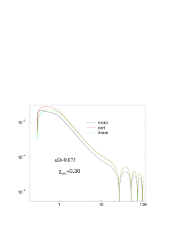
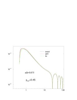
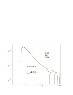
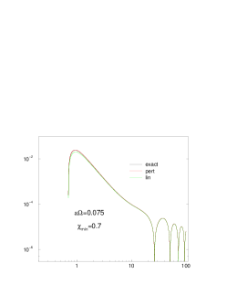
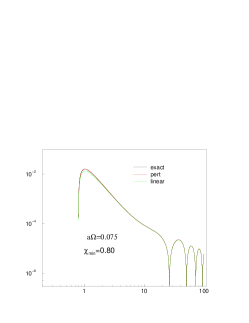
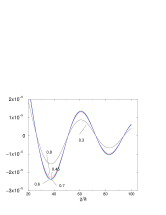
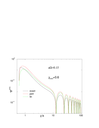
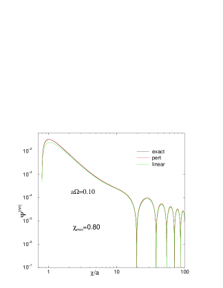
Table 1 gives a crude analysis of the correlation of the field strength at the inner boundary and the agreement of the three computations for a given model. The parameters of the model are given in columns two and three with the fourth column giving the estimate of the field strength at the inner boundary, according to the criterion in Eq. (106). The remaining columns give various indicators of agreement of the linearized, PPM, and Exact PM computations.
In the near zone the comparison is done by using differences in the value of the first maximum of near the inner boundary; this is the maximum of each of the curves of Figs. 1 and 3. (The value at the inner boundary itself is fixed by the boundary conditions. At the inner boundary, therefore, the results for PPM and Exact PM must be the same; the difference between these two and the linearized computation would only reveal the second order difference in the bounary values used.) The columns labeled “Lin v. PPM” gives the fractional difference of the computed value of this maximum for the linearized and the PPM computation. The column “PPM v. Exact” does the same for the two second-order post-Minkowski computations. The following two columns test the hypothesis that the difference between the linearized and the PPM results are second-order in the boundary-value field strength, and that the PPM vs. Exact PM results are third order. If those order estimates were accurate, the numerical values in columns seven and eight would be expected to have little variation. Columns nine through twelve give the same indicators as those in five through eight, but now for the wave zone. In the wave zone the criterion for agreement is taken to be the maximum of the first wave, e.g. , at in the plot for the , model in Fig. 3.
| near zone | wave zone | ||||||||||
| Lin v. | PPM v | Lin/PPM | Lin/Exact | Lin v. | PPM v | Lin/PPM | Lin/Exact | ||||
| model | PPM | Exact | PPM | Exact | |||||||
| Ia | 0.075 | 0.3 | 0.5 | 0.61 | 0.67 | 2.4 | 5.3 | .031 | 0.85 | 0.12 | 6.8 |
| Ib | 0.075 | 0.45 | 0.222.. | 0.34 | 0.10 | 6.9 | 9.1 | .03 | 0.18 | 0.61 | 16.4 |
| Ic | 0.075 | 0.6 | 0.125 | 0.24 | 0.006 | 15 | 2.9 | .032 | 0.64 | 2.0 | 33 |
| Id | 0.075 | 0.7 | 0.0918 | .20 | 0.0016 | 24 | 2.1 | .03 | 0.03 | 3.6 | 39 |
| Ie | 0.075 | 0.8 | 0.0703 | 0.17 | 0.006 | 34 | 18 | .029 | 0.020 | 6 | 58 |
| II | 0.100 | 0.8 | 0.125 | 0.31 | 0.019 | 20 | 9.7 | .067 | 0.063 | 4 | 32 |
| III | 0.150 | 0.6 | 0.5 | 1.0 | 0.36 | 4 | 2.9 | .23 | 1.0 | 9 | 8 |
The values in Table 1, for the near zone, show weak evidence for the expected effects of the field strength at the inner boundary The values in the wave zone show less evidence and, along with Fig. 2, suggest that the error in the wave zone tends not to be dominated by the location of .
The lack of clear evidence of field-strength effects is not a complete surprise. For large values of , the field strength for these models, we should expect the post-Minkowski approximation to be too crude. The disagreements on the order of 100% are in accord with this, and an analysis based on orders of a small parameter should fail. For significantly smaller values of the error induced by the location of are small, and other sources of error dominate.
V Summary and conclusions
In this paper we present methods and results for the post-Minkowski level of computations within the Periodic Standing Wave approximation. More specifically, we present the theoretical background for the PM computations along with two distinct ways of computationally treating the second-order PM equations: (i) the perturbative PM method in which first-order fields are initially computed and used as sources in the linear equations for the second order fields, and (ii) the exact PM method in which the second-order PM equations are solved as if they constituted an exact theory.
Although the present paper deals with the second-order PM approximation, the full equations of general relativity, in the harmonic gauge, were given in a form easily adaptable to helical symmetry. In fact, an important point made in the paper is that the computational structure of the exact PM problem differs very little from that of full general relativity.
In the development of the infrastructure for for the problem, we showed the utitility of the formalism of the helically symmetric complex field projections , introduced earlier for linearized gravity theorylineareigen . That formalism serves well not only for the second-order PM work, but also for full general relativity.
The details of the mathematical description of fields and motions clarify the difference between the PM approximation for a binary system and a post-Newtonian approximation for that system. At a characterisitic distance from one of the sources, the gravitational field strength is of order . Our PM approximation demands that , since it was the very smallness of this term that justifies omitting higher order terms in the PM approximation. The PM approximation then, in a sense, is an approximation focused on the near-source fields. By contrast, the post-Newtonian approximation is one in which the source velocity is small compared to , or . In a very relativistic black hole binary, one in which the two holes are almost in contact, there is no significant difference between and . But the PSW approximation makes no sense unless is an order or magnitude or more.
Thus, in our equations, we can distinguish the approximations associated with field strength and with small velocity, and we find it useful to do this. The limitation of field strength, that associated with the PM approximation, is determined by the value of at the inner boundary. The parameter for the post-Newtonian approximation, by contrast, is simply . In our computations we consider values of that are not exceedingly small, such as the models of Table 1. We may, at the same time, keep terms that are second order in , though these terms may be orders of magnitude smaller than 0.5. The choice we have made in this paper is to keep terms to second order both in and in . These distinctions will become even more important in the PSW approximation for full general relativity.
An important aspect of the present paper is that it shows that there are no insurmountable computational difficulties in computing the post-Minkowski PSW fields. This more-or-less guarantees that there will be no significant computational difficulties in the PSW problem in full general relativity, as long as we choose the inner boundary sufficiently large. The computational challenge for the full general relativity problem will be in dealing with the strong fields in the case that is chosen small enough to give a good representation of conditions very near a black hole. The full general relativity problem will, of course, also entail interesting issues of interpretation.
Lastly, the fact that we can now compute second-order PM fields means that, in principle, our results can be used as trial initial conditions for numerical evolution codes. In practice, our results are limited to the region , and evolution codes require data also for . The obvious first attempt at a remedy to this is to glue a pure Schwarzschild puncture into the region.
VI Acknowledgment
We gratefully acknowledge the support of NSF grants PHY 0400588, PHY 0555644, PHY 0514282 and PHY 0554367, and NASA grant ATP03-0001-0027. We thank Kip Thorne, Lee Lindblom, Mark Scheel and the Caltech numerical relativity group, and John Friedman for many useful discussions and suggestions.
Appendix A Details of the First Order Driving Term
Here we give the details of the terms on the right in Eq. (90). We start with the Einstein equations truncated to second order, as given in Eq. (34), and we write this equation as
| (110) |
As argued in Sec. II.2, only the terms have a nonzero first-order part, so only these need appear on the right, and the driving term on the right in Eq. (110) simplifies to
| (111) |
where
| (112) |
We next substitute , from Eq. (74), on the left in Eq. (111) and use the fact that , to get
| (113) |
We can now use the fact that the basis tensors have the following orthogonality property under contraction and complex conjugation
| (114) |
where
| (115) |
Using this, we contract Eq. (113) with to get
| (116) | ||||
Multiplying by puts this in the form of Eq. (76), and we conclude
| (117) |
This result gives in terms of derivatives of the fields with respect to the Minkowski-like fundamental coordinates. What is needed is the form indicated in Eq. (81): derivatives of the fields with respect to the adapted coordinates. The change to this form requires two transformations. First, the derivatives with respect to the four Minkowski-like coordinates must be changed to derivatives with respect to the rotating coordinates . In doing this, helical symmetry is imposed by using Eq. (9) to replace . The fact that has been constructed to be a helical scalar guarantees that there will be no explicit time dependence in Eq. (117); will be a function only of rotating coordinates. How this comes about is related to the fact that so that
| (118) |
As an explicit example, here we evaluate . The general expression in Eq. (118) becomes
| (119) |
[Recall that .] It is simplest to use the basis for evaluation. From the definition in Eqs. (66) we have that and so that
| (120) | ||||
where the time derivative of has been replaced following the helical prescription of Eq. (9)
It is convenient next to reexpress the results in terms of the rotating coordinates in which the axis is aligned with the sources, rather than the rotational axis. For our example, this gives
| (121) |
Finally we can convert the derivatives with respect to to derivatives with respect to the adapted coordinates by using the following relationships (see Refs. eigenspec ,lineareigen ). With the definitions
| (122) |
the partial derivatives for transforming to adapted coordinates take the fairly simple form
| (123) |
| (124) |
| (125) |
| (126) |
| (127) |
| (128) |
| (129) |
| (130) |
| (131) |
The first factor in our example in Eq. (121) has already appeared in Eq. (93):
| (132) |
The coefficients, given in the appendix of Ref. lineareigen , are
| (133) |
| (134) |
| (135) |
References
- (1) M. Campanelli, C. O. Lousto, P. Marronetti, and Y. Zlochower, Phys. Rev. Lett. 95, 111101 (2006); M. Campanelli, C. O. Lousto, and Y. Zl ochower, Phys. Rev. D 73 061501(R) (2006).
- (2) J. G. Baker, J. Centrella, D.-I. Choi, M. Koppitz, and J. van Meter, 96, 121102 (2006).
- (3) J. T. Whelan, W. Krivan, and R. H. Price, Class. Quant. Grav. 17, 4895 (2000).
- (4) J. T. Whelan, C. Beetle, W. Landry, and R. H. Price, Class. Quant. Grav. 19, 1285 (2002).
- (5) R. H. Price, Class. Quant. Grav. 21, S281 (2004).
- (6) Z. Andrade et al., Phys. Rev. D 70, 064001 (2004).
- (7) B. Bromley, R. Owen and R. H. Price Phys. Rev. D71, 104017 (2005).
- (8) C. Beetle, B. Bromley, and R. H. Price, Phys Rev D vol 74, 024013 (2006).
- (9) C. Beetle, paper in preparation.
- (10) C. W. Misner, K. S. Thorne and J. A. Wheeler, Gravitation (Freeman, San Francisco, 1973).
- (11) L. D. Landau and E. M. Lifschitz, The Classical Theory of Fields, translated by M. Hamermesh, (Addison-Wesley, Reading Mass., 1962), Sec. 100.
- (12) Ref. MTW , Sec. 20.3.
- (13) C. R. Johnson, Phys. Rev. D4, 295 (1971); Phys. Rev. D4, 318 (1971); Phys. Rev. D4, 3555 (1971); Phys. Rev. D5, 1916 (1972).
- (14) J. Van Meter, unpublished PhD thesis, University of California, Davis, 1999.
- (15) S. Weinberg, Gravitation and Cosmology: Principles and Applications of the General Theory of Relativity, (John Wiley and Sons, New York, 1972), p. 181.
- (16) The coordinates here have no relations to the Minkowski coordinates used in Refs. paperI ; eigenspec ; lineareigen .
- (17) That such a path is appropriate (i.e. , is a geodesic) is inherent in the helical symmetry that is assumed for the solution, and the form of the helical Killing vector given in Eq. ( 6).
- (18) Ref. MTW , Sec. 18.1.