Low-power radio galaxy environments in the Subaru/XMM-Newton Deep Field at $\mathbf{z\sim 0.5}$

Abstract

We present multi-object spectroscopy of galaxies in the immediate (Mpc-scale) environments of four low-power ($L_{\rm 1.4GHz}\lesssim 10^{25}$ W Hz^-1) radio galaxies at $z\sim 0.5$, selected from the Subaru/XMM-Newton Deep Field. We use the spectra to calculate velocity dispersions and central redshifts of the groups the radio galaxies inhabit, and combined with XMM-Newton (0.3–10 keV) X-ray observations investigate the $L_{X}$–$\sigma_{v}$ and $T_{X}$–$\sigma_{v}$ scaling relationships. All the radio galaxies reside in moderately rich groups – intermediate environments between poor groups and rich clusters, with remarkably similar X-ray properties. We concentrate our discussion on our best statistical example that we interpret as a low-power (FR I) source triggered within a sub-group, which in turn is interacting with a nearby group of galaxies, containing the bulk of the X-ray emission for the system – a basic scenario which can be compared to more powerful radio sources at both high ($z>4$) and low ($z<0.1$) redshifts. This suggests that galaxy-galaxy interactions triggered by group mergers may play an important role in the life-cycle of radio galaxies at all epochs and luminosities.

1 Introduction

Table 1: Summary of radio galaxy targets. I.D.’s, positions and fluxes are taken from an early version of the 1.4 GHz Very Large Array radio mosaic presented in Simpson et al. 2006 (S06). In this paper for convenience we shortern IAU identifications of the radio galaxies to JEG 1–4. We quote radio luminosities here for completeness, however we discuss the redshift determination in §3.2.

I.D.	IAU I.D.	S06 I.D.	R.A.	Dec.	$S^{\rm SXDF}_{1.4\rm\,GHz}$	$L_{1.4\rm\,GHz}$
			(J2000.0)	(J2000.0)	(mJy)	($10^{24}$ W Hz-1)
JEG 1	VLA J021945$-$04535	$-$	02 19 45.3	$-$04 53 33	11.86$\pm$0.13	4.36$\pm$0.05
JEG 2	VLA J021823$-$05250	VLA 0011	02 18 23.5	$-$05 25 00	7.95$\pm$0.10	14.35$\pm$0.18
JEG 3	VLA J021737$-$05134	VLA 0033	02 17 37.2	$-$05 13 28	2.37$\pm$0.06	4.26$\pm$0.11
JEG 4	VLA J021842$-$05328	VLA 0065	02 18 42.1	$-$05 32 51	0.96$\pm$0.08	0.48$\pm$0.04

Figure 1: $R-z^{\prime}$ vs. $z^{\prime}$ Field-corrected colour-magnitude diagrams for each mask. Photometry was extracted from the SXDF catalog by choosing all galaxies within an aperture of radius 2.5^′ centered on the brightest target galaxy. Colours are measured in 2^′′ apertures, and we also indicate a secondary colour, $i^{\prime}-z^{\prime}$ (arbitrarily chosen), to emphasise the location of the red-sequence as larger points. The colours of targeted galaxies in this work are indicated by larger open circles.

In recent years, feedback mechanisms from radio galaxies (that is, galaxies which host radio-loud active galactic nuclei) have become the method of choice for curtailing the bright end of the galaxy luminosity function in models of galaxy formation, since models without feedback tend to over-produce the number of very luminous galaxies compared to what is observed (e.g. Bower et al. 2006). Many high-redshift radio galaxies lie in (proto-)cluster environments (e.g. Venemans et al. 2003) and the energies provided by their radio jets (the bulk kinetic power of the radio jets is several orders of magnitude larger than the radio luminosity; e.g., Rawlings & Saunders 1991) is sufficient to shut down star forming activity throughout a cluster (Rawlings & Jarvis 2004). Furthermore, it has been suggested that powerful radio sources may be triggered by galaxy–galaxy interactions during the merging of subcluster units (Ellingson, Yee & Green 1991; Simpson & Rawlings 2002).

Lower luminosity sources are also believed to be vital in shaping the galaxy luminosity function by providing a low power, but high duty cycle, mode of feedback (e.g., Croton et al. 2005; Bower et al. 2006; Best et al. 2006). This mode of feedback appears to be most common in the most massive galaxies, which are, of course, preferentially located in the centres of galaxy clusters. Therefore there appears to be significant interplay between the formation and evolution of both the radio sources and their cluster environments. Studying the environments of low-power radio sources is likely a promising route towards understanding radio galaxy feedback. However, while the radio galaxy itself can influence the thermodynamic history of its environment (i.e. by depositing energy), the picture is complicated by global environmental processes such as the merging of sub-cluster units, which can temporarily boost the X-ray luminosity and temperature of the intracluster medium (e.g. Randall, Sarazin & Ricker 2002), making such systems more readily detectable in X-ray surveys (a matter of caution in using such X-ray detected systems as Cosmological probes). It is essential to perform detailed studies of the radio, optical, and X-ray properties of putative dense regions in the cosmic web to ascertain how mergers and radio source activity affect the life-cycle of clusters.

The luminosity and temperature of a cluster are known to follow a scaling relationship (the $L_{X}$–$T_{X}$ relation), $L_{X}\propto T_{X}^{\alpha}$, where $\alpha$ has been measured in the range $\sim$2.7–3 (Edge & Stewart 1991; David, Jones & Forman 1995; Allen & Fabian 1998; Markevitch 1998; Arnaud & Evrard 1999) This is at odds with that expected for clusters formed by gravitational structure formation, with $L_{X}\propto T_{X}^{2}$ (Kaiser 1986). It is thought that the disparity is due to the interruption of cooling by feedback from active galaxies, which can impart energy via outflow shocks (for example from radio-jets or super-winds), or by performing work by sub-sonically inflating bubbles in the intracluster medium (ICM; Sijacki & Springel 2006). Best et al. (2005) suggest that, given the short life-times of radio-loud AGN (10–100 Myr), episodic triggering must occur in order for feedback to quench cooling. However, much lower luminosity sources ($L_{\rm 1.4\,GHz}<10^{25}$ W Hz^-1) can impart energy into the IGM with a higher duty cycle than the more powerful, and rarer, sources (Best et al. 2006).

McLure et al. (2004) have recently constructed a sample of radio galaxies at $z\sim 0.5$ which spans three orders of magnitude in radio luminosity, but even the faintest of these sources are close to the Fanaroff–Riley break (Fanaroff & Riley 1974) and it is desirable to push to even fainter radio luminosities to fully investigate the radio galaxy–cluster symbiosis. In this paper we present multi-object spectroscopy of galaxies around four low-power ($L_{\rm 1.4\,GHz}<10^{25}$ W Hz^-1) radio galaxies at $z\sim 0.5$ in the Subaru/XMM-Newton Deep Field (SXDF) (Sekiguchi et al. 2001, 2006 in prep). The resultant spectroscopic redshifts allow us to investigate the environments of these radio sources which could provide a large proportion of the local volume averaged heating rate if the AGN luminosity function is flat below $L_{\rm 1.4\,GHz}\sim 10^{25}$ W Hz^-1 (Best et al. 2006). We combine these data with X-ray observations of the radio galaxies’ environments in order to investigate the global environmental properties – namely the $L_{X}-\sigma_{v}$ and $T_{X}-\sigma_{v}$ relations. This parameter space can be used as a diagnostic of the thermodynamic history of groups or clusters, since if an AGN is significantly feeding energy back into the intracluster medium (ICM), then the group or cluster might be expected to deviate from the standard empirical $L_{X}(T_{X})-\sigma_{v}$ relation for massive systems. Throughout we adopt a flat geometry with $\Omega_{\rm m}=0.3$, $\Omega_{\Lambda}=0.7$ and $H_{0}=100h$ km s^-1 Mpc^-1 where $h=0.75$. All magnitudes in this paper are on the AB scale.

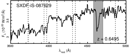
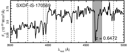
Figure 2: Successfully cross-correlated spectra for the radio galaxies field of (top-down) JEG 1–4. The spectra are plotted in the rest-frame. As a guide, we identify as dotted vertical lines the spectral features [Oii], K, H, H$\delta$, G, H$\gamma$, and H$\beta$. We do not plot wavelengths blueward of 3500Å or redward of 5000Å (restframe) since in these regimes the response and signal-to-noise of the spectra do not allow accurate analysis. Note that the shaded region highlights a sky absorption feature.

2 Observations & Reduction

2.1 Sample selection and spectroscopy

Targets were selected from an early version of the 1.4-GHz Very Large Array radio mosaic presented in Simpson et al. (2006), and listed in Table 1. The limited red sensitivity of the Low Dispersion Survey Spectrograph (LDSS-2, Allington-Smith et al. 1994) placed an upper limit of $z\sim 0.7$ as appropriate for our study, so we selected radio sources whose optical counterparts are resolved and have $19<R<20.5$, since the tightness of the Hubble diagram for radio galaxies allows redshifts to be estimated from a single magnitude, and we aim to target moderate redshift environments (Cruz et al. 2007). Colour–magnitude diagrams were produced for $2.5^{\prime}$ regions around each radio galaxy and the four optically brightest radio galaxies whose environments displayed a red sequence were selected for spectroscopic follow-up. This selection was simply performed ‘by eye’ – if the colour-magnitude diagram displayed an overdensity of points at $18<m_{\rm RG}<20.5$ with tight scatter in colour space. Note that local X-ray properties were not taken into account when choosing the target radio galaxies – this is simply an optical selection of radio galaxies.

Masks were designed using the LDSS-2 mask preparation software, with objects along the red sequence (typically using a colour cut of width 0.3 magnitudes) included in the input file (Figure 1). This software allows relative priorities to be assigned to targets, which were set to be equal to the magnitudes of the galaxies, to increase the likelihood of successfully determining redshift.

Observations were conducted using the medium-red (300 lines/mm, $\lambda_{0}=5550$Å) grism of LDSS-2 in multi-object mode on the 6.5-m Magellan telescope in Las Campanas, Chile over the nights 17–20 October 2003 (effective resolution 13.3Å). The MOS frames were trimmed for overscan, flat-fielded, rectified, cleaned and wavelength calibrated using a sequence of Python routines (D. Kelson, priv. comm.); sky-subtraction and spectrum extraction was performed in IDL. Due to a lack of standard-star observations, for flux-calibration and to correct for the wavelength dependent response of the detector, we extracted BVRi^′z^′ photometry for the targets from the Subaru/XMM-Newton Deep Field (SXDF) catalog. Using the five sources in each mask with the strongest signal-to-noise ratio (SNR), we fit mask-specific response curves to the 1-D spectra, which are then applied to each extracted target spectrum. Although flux-calibration and response correction is not necessary for redshift determination via cross-correlation, we perform these steps in order to present a sample of the spectra in Figure 2.

2.2 X-ray data

The SXDF incorporates a deep, large-area X-ray mosaic with XMM-Newton, consisting of 7 overlapping pointings covering $\sim$1.3 deg² region of the high-Galactic latitude sky with an exposure time of 100 ks in the central field (in separate exposures) and 50 ks in the flanking fields (see Table 2). Four of the pointings were carried out in August 2000, and the remaining three were made in August 2002 and January 2003.

Table 2: Overview of the XMM-Newton observations. Tabulated are the Field IDs, the centres of the pointings and the exposure times of the relevant high-background-cleaned datasets for each camera: MOS 1, MOS 2 and PN. Note that the coordinates are in J 2000.

Field	R.A.	Dec.	Exp. time [MOS 1  MOS 2  PN]
	hh  mm  ss	$\circ$  ′  ′′	(ksec)
SDS-1a	02 18 00	$-$05 00 00	$-$  $-$  40
SDS-1b	02 18 00	$-$05 00 00	$-$  $-$  42
SDS-2	02 19 36	$-$05 00 00	47  48  40
SDS-6	02 17 12	$-$05 20 47	49  49  47
SDS-7	02 18 48	$-$05 20 47	40  41  35

All the XMM-Newton EPIC data, i.e. the data from the two MOS cameras and the single PN camera, were taken in full-frame mode with the thin filter in place. These data have been reprocessed using the standard procedures in the most recent XMM-Newton SAS (Science Analysis System) $-$ v.6.5. All the datasets where at least one of the radio galaxies was seen to fall within the field-of-view (FOV) of the detectors were then analysed further. JEG 3 was observed in pointings SDS-1a (PN), SDS-1b (PN) and SDS-6 (M1, M2, PN) (part of the field lies off the edge of the MOS FOVs in SDS1a and SDS1b). Both JEG 2 and JEG 4 were observed in pointing SDS-7 (MOS 1, MOS 2, PN). Finally JEG 1 was observed in pointing SDS-2 (MOS 1, MOS 2, PN). Periods of high-background were filtered out of each dataset by creating a high-energy 10$-$15 keV lightcurve of single events over the entire field of view, and selecting times when this lightcurve peaked above 0.75 ct s^-1 (for PN) or 0.25 ct s^-1 (for MOS). It is known that soft proton flares can affect the background at low energies at different levels and times than high energies (e.g. Nevalainen et al. 2005). This was not seen to be the case in the datasets analysed here however, as full energy-band (1–10 keV) lightcurves (extracted from off-source regions) showed essentially identical times of flaring activity as the high energy lightcurves. The high-background times in each dataset are seen to be very distinct and essentially unchanging with energy-band. The exposure times of the resulting cleaned relevant datasets are given in Table 2.

Source spectra were extracted from the relevant datasets from apertures centred on the source positions. Extraction radii, estimated from where the radial surface brightness profiles were seen to fall to the general surrounding background level, were set to 50^′′, 21^′′, 36^′′ and 47^′′ for JEG 1–4 respectively. Note that the surface brightness profiles were co-added for all 3 EPIC cameras for improved S/N. Standard SAS source-detection algorithms, uncovered a large number of X-ray sources, both point-like and extended. Data due to contaminating sources lying within the extraction regions needed to be removed from the spectra. This proved necessary only for JEG 3, where two sources were detected just within the extraction region. Data from the two sources were removed to a radius of 28^′′ (and the extraction area is thus reduced by $\sim 10$%). Background spectra were extracted from each cleaned dataset from an annulus of inner radius 60^′′ and outer radius 180^′′ around each position. As point sources were seen to contaminate these larger-area background spectra, the data from these detected sources were removed from the background spectra to a radius of 60^′′. We have verified that all the X-ray sources are clearly extended using both simple (sliding box) and more sophisticated wavelet analysis techniques. The possibility that JEG 2 is an unresolved source complex cannot of course be completely ruled out given its low signal to noise. Given the relative weakness of all of the X-ray sources, we consider that the extraction radii used are close to optimum to provide the best signal to noise in the extracted spectra. Ancillary Response Files (ARFs) containing the telescope effective area, filter transmission and quantum efficiency curves were created for the cluster spectra (taking into account the fact that the extraction regions are extended), and were checked to confirm that the correct extraction area calculations (complicated with the exclusion of contaminating point sources, etc.) had been performed. Finally Redistribution Matrix Files (RMFs) files were generated. These files describe, for a given incident X-ray photon energy, the observed photon energy distribution over the instrument channels. These can be used in conjunction with the ARFs to perform X-ray spectral analysis – we use the most commonly used analysis package: xspec. The source spectral channels were binned together to give a minimum of 20 net counts per bin. A detailed discussion of the X-ray spectral fitting and the results is given in §3.4

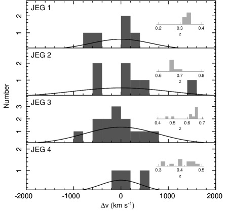
Figure 3: Relative velocity distribution of galaxies where successful redshift-determination was performed. Relative velocities are in the cluster frame, over a range $\pm 2000$ km s^-1. Insets show the distribution in redshift space, over a wider velocity range. We overlay Gaussian profiles based on the fitted velocity dispersion in each case.

3 Analysis

3.1 Colour-magnitude diagrams

In Figure 1 we plot the $R-z^{\prime}$ vs. $z^{\prime}$ colour-magnitude relations (CMRs) for each field, which have been constructed from the photometry of all galaxies within 2.5^′ of each radio-galaxy target. We correct the colour-magnitude diagrams for field contamination using a method similar to Kodama et al. (2004) and Kodama & Bower (2001), which we will briefly describe here. First, colour-magnitude space is divided into a coarse grid ($\Delta z^{\prime}=2$, $\Delta(R-z^{\prime})=0.8$), and the number of galaxies within each grid-square counted: $N^{\rm gal}_{ij}$. An identical count is performed for a control field, $N^{\rm control}_{ij}$, where control galaxies are selected within an aperture of identical radius to the one used for each target mask, but centered on a random point on the sky (but within the catalog). We then assign the $ij^{\rm th}$ colour-magnitude bin the probability that the galaxies within it are field members: $P_{ij}=N^{\rm control}_{ij}/(N^{\rm gal}_{ij}+N^{\rm control}_{ij})$. For each galaxy in colour-magnitude space, we pick a random number, $p$, in the interval {0,1} and compare it to $P_{ij}$; a galaxy is removed from the diagram if $p<P_{ij}$. In order to reduce effects of cosmic-variance (e.g. randomly picking another cluster or void as the control sample), we build up an average probability map by repeating the control sample count and probability calculation 10 times around different random positions in the catalog.

There are clear red-sequences around all four radio galaxies, and to emphasise this, we also plot a secondary colour $i-z^{\prime}$, and the locations of galaxies in colour space targeted for spectroscopy. The secondary colour-cut is chosen merely to highlight the red-sequence.

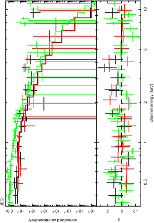
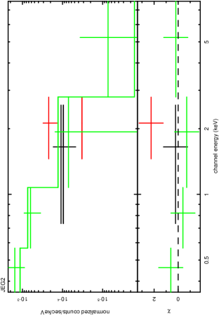
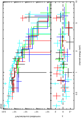
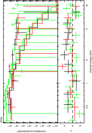
Figure 4: The XMM-Newton EPIC spectra of (row-wise from top left) JEG 1–4, together with the best-fitting thermal plasma model fitted using xspec. $\chi^{2}$ differences are shown in the lower panels of each plot. The colour-codings correspond to the MOS 1, MOS 2 and PN cameras and field pointings (see Table 2 and §2.2). For JEG 1 (SDS-2), JEG 2 (SDS-7) & JEG 4 (SDS-7) black is MOS 1, red is MOS 2 and green is PN. For JEG 3 black is PN (SDS-1a), red is PN (SDS-1b), green is MOS 1 (SDS-6), blue is MOS 2 (SDS-6) and cyan is PS (SDS-6). The resulting cluster parameters of $L_{X}$ and $T_{X}$ are presented in Table 4.

3.2 Redshift determination and velocity dispersions

For redshift determination we use the velocity code of Kelson et al. (D. Kelson, priv. comm.), which cross-correlates target and template spectra. The errors are determined from the topology of the cross-correlation peak (i.e. the width of a Gaussian profile fit to the peak in the cross-correlation spectrum) and the noise associated with the spectrum; typically in the range 30–210 km s^-1. We present spectra of the target radio galaxies which have been successfully cross-correlated and shifted to the rest-frame in Figure 2. In Table 3 we list the coordinates, $z^{\prime}$ magnitudes and redshifts of successfully cross-correlated targets, with the radio galaxies highlighted.

To calculate the velocity dispersions of each cluster, we follow the iterative method used by Lubin, Oke & Postman (2002) and others (e.g. Willis et al. 2005). Initially we estimate that the cluster central redshift is that of the target radio galaxies, and select all other galaxies with $|\Delta z|<0.06$ in redshift space. We then calculate the biweight mean and scale of the velocity distribution (Beers, Flynn & Gebhardt 1990) which correspond to the central velocity location, $v_{c}$, and dispersion, $\sigma_{v}$ of the cluster. We can use this to calculate the relative radial velocities in the cluster frame: $\Delta v=c(z-z_{c})/(1+z_{c})$. The original distribution is revised, and any galaxy that lies $>$3$\sigma_{v}$ away from $v_{c}$, or has $|\Delta v|>$ 3500 km s^-1 is rejected from the sample and the statistics are re-calculated. The final result is achieved when no more rejection is necessary, and the velocity dispersion and cluster redshift can be extracted. The results are presented in Table 4, with 1-$\sigma$ errors on the cluster redshift and dispersion corresponding to 1000 bootstrap resamples of the redshift distribution.

In Figure 3 we plot the redshift distribution of those galaxies for which we performed successful cross-correlations. We also plot the velocities of those galaxies within $|\Delta v|<2000$ km s^-1 of the cluster central redshift, overlaid with standard Gaussian profiles. JEG 3 is the largest sample of cluster galaxies (in part due to the large number of galaxies targeted in this field). JEG 1 and JEG 4 (at similar redshifts) have relatively few members after the process of rejection described above. JEG 2 has a high velocity dispersion, indicating a non-relaxed system, despite the fairly prominent red-sequence in this region. In part, the high velocity dispersion might be attributed to an outlying galaxy in the velocity distribution, but as we discuss in §3.3, JEG 2 might be part of a larger, more complicated stucture than a simple group.

Table 3: Spectroscopic targets with total $z^{\prime}$ band magnitudes and cross-correlated redshifts. Redshift uncertainties are derived from the topology of the cross-correlation peak. The radio galaxy is highlighted in bold type in each case.

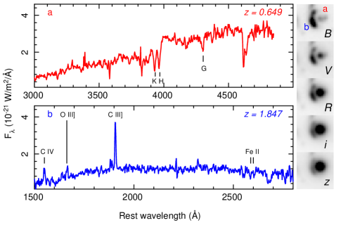
Figure 7: Spectra of components ‘a’ and ‘b’ of the radio galaxy in the field of JEG 3 – SXDF-iS-170569. The inset greyscale images are $6^{\prime\prime}\times 6^{\prime\prime}$ Subaru SuprimeCam thumbnails in $BVRiz$ bands, clearly showing the distinction between a red component ‘a’ and blue component ‘b’. The spectra unambiguously identify ‘b’ with a galaxy at $z=1.847$, strongly lensed by the foreground component ‘a’. The emission lines at the very blue end of the spectrum ‘b’ are Civ, Oiii] and Ciii] in emission, securing the redshift. Fe III is seen in absorption at 2587Å and 2600Å.

I.D.	RA	Dec.	$z^{\prime}$	Redshift	Member⋆
	(J2000.0)	(J2000.0)	(mag)
JEG 1
SXDF-iE-085449	02:19:45.252	$-$04:53:33.08	18.27	0.3333${}^{+0.0001}_{-0.0001}$	$\bullet$
SXDF-iE-079345	02:19:39.461	$-$04:53:18.56	18.83	0.3029${}^{+0.0002}_{-0.0004}$	$\circ$
SXDF-iE-073826	02:19:36.864	$-$04:53:29.98	18.01	0.3038${}^{+0.0001}_{-0.0001}$	$\circ$
SXDF-iE-094234	02:19:48.300	$-$04:53:23.65	19.56	0.3297${}^{+0.0001}_{-0.0001}$	$\bullet$
SXDF-iE-089522	02:19:46.118	$-$04:51:22.25	19.36	0.3302${}^{+0.0002}_{-0.0001}$	$\bullet$
SXDF-iE-085293	02:19:43.190	$-$04:52:43.50	19.33	0.3336${}^{+0.0001}_{-0.0001}$	$\bullet$
SXDF-iE-067505	02:19:33.689	$-$04:51:45.47	18.35	0.3059${}^{+0.0001}_{-0.0001}$	$\circ$
SXDF-iE-080550	02:19:41.508	$-$04:52:30.60	17.61	0.3329${}^{+0.0001}_{-0.0001}$	$\bullet$
JEG 2
SXDF-iS-087629	02:18:23.532	$-$05:25:00.65	19.17	0.6495${}^{+0.0001}_{-0.0002}$	$\bullet$
SXDF-iS-105254	02:18:19.109	$-$05:23:06.32	20.02	0.6515${}^{+0.0002}_{-0.0003}$	$\bullet$
SXDF-iS-100288	02:18:19.066	$-$05:23:45.74	20.19	0.6812${}^{+0.0004}_{-0.0005}$	$\circ$
SXDF-iS-111951	02:18:20.074	$-$05:22:14.13	21.49	0.6748${}^{+0.0003}_{-0.0005}$	$\circ$
SXDF-iS-108679	02:18:20.374	$-$05:22:36.40	20.64	0.6566${}^{+0.0002}_{-0.0004}$	$\bullet$
SXDF-iS-087515	02:18:23.777	$-$05:25:49.89	21.73	0.6459${}^{+0.0002}_{-0.0002}$	$\bullet$
SXDF-iS-090262	02:18:26.772	$-$05:25:14.35	19.66	0.6502${}^{+0.0001}_{-0.0002}$	$\bullet$
SXDF-iS-070840	02:18:27.202	$-$05:27:36.30	19.70	0.6488${}^{+0.0002}_{-0.0003}$	$\bullet$
SXDF-iS-102854	02:18:29.954	$-$05:23:30.49	20.73	0.6456${}^{+0.0005}_{-0.0005}$	$\bullet$
JEG 3
SXDF-iS-170569	02:17:37.193	$-$05:13:29.61	19.30	0.6472${}^{+0.0004}_{-0.0004}$	$\bullet\dagger$
SXDF-iS-157505	02:17:24.230	$-$05:15:19.53	19.76	0.6506${}^{+0.0001}_{-0.0002}$	$\bullet$
SXDF-iS-173222	02:17:26.530	$-$05:13:45.93	21.01	0.6516${}^{+0.0001}_{-0.0001}$	$\bullet$
SXDF-iS-182658	02:17:27.502	$-$05:11:45.34	21.44	0.6484${}^{+0.0001}_{-0.0001}$	$\bullet$
SXDF-iS-168040	02:17:29.052	$-$05:12:59.61	19.89	0.6494${}^{+0.0001}_{-0.0001}$	$\bullet$
SXDF-iS-154410	02:17:33.286	$-$05:15:51.00	19.46	0.6027${}^{+0.0001}_{-0.0001}$	$\circ$
SXDF-iS-184999	02:17:31.322	$-$05:12:17.11	20.85	0.6010${}^{+0.0001}_{-0.0001}$	$\circ$
SXDF-iS-172233	02:17:35.309	$-$05:13:30.71	19.76	0.6495${}^{+0.0003}_{-0.0003}$	$\bullet$
SXDF-iS-172341	02:17:43.358	$-$05:13:30.69	20.78	0.6470${}^{+0.0001}_{-0.0001}$	$\bullet$
SXDF-iS-172053	02:17:34.202	$-$05:13:39.44	19.36	0.4464${}^{+0.0002}_{-0.0002}$	$\circ$
SXDF-iS-181772	02:17:25.450	$-$05:11:54.43	19.81	0.6274${}^{+0.0002}_{-0.0002}$	$\circ$
SXDF-iS-169690	02:17:26.858	$-$05:13:16.88	21.17	0.6481${}^{+0.0001}_{-0.0002}$	$\bullet$
SXDF-iS-166516	02:17:31.070	$-$05:12:37.74	21.17	0.6522${}^{+0.0001}_{-0.0001}$	$\bullet$
SXDF-iS-167467	02:17:32.566	$-$05:12:59.88	19.85	0.6433${}^{+0.0001}_{-0.0001}$	$\bullet$
SXDF-iS-178431	02:17:35.803	$-$05:14:20.76	20.82	0.6475${}^{+0.0002}_{-0.0002}$	$\bullet$
SXDF-iS-163351	02:17:37.512	$-$05:14:31.25	20.15	0.6455${}^{+0.0002}_{-0.0002}$	$\bullet$
SXDF-iS-172154	02:17:46.733	$-$05:13:35.17	21.33	0.6456${}^{+0.0007}_{-0.0005}$	$\bullet$
SXDF-iS-131866	02:17:31.500	$-$05:19:26.34	23.43	0.4943${}^{+0.0002}_{-0.0002}$	$\circ$
JEG 4
SXDF-iS-037426	02:18:42.067	$-$05:32:51.03	18.76	0.3832${}^{+0.0001}_{-0.0001}$	$\bullet$
SXDF-iS-029867	02:18:32.484	$-$05:34:21.33	20.46	0.4238${}^{+0.0002}_{-0.0002}$	$\circ$
SXDF-iS-049475	02:18:34.486	$-$05:31:28.97	20.51	0.4275${}^{+0.0002}_{-0.0001}$	$\circ$
SXDF-iS-048741	02:18:35.635	$-$05:31:33.23	20.29	0.3126${}^{+0.0003}_{-0.0008}$	$\circ$
SXDF-iS-035961	02:18:37.447	$-$05:32:49.61	18.60	0.4576${}^{+0.0001}_{-0.0001}$	$\circ$
SXDF-iS-041384	02:18:38.986	$-$05:32:38.25	19.46	0.4725${}^{+0.0002}_{-0.0002}$	$\circ$
SXDF-iS-029332	02:18:40.183	$-$05:34:01.32	19.31	0.4588${}^{+0.0001}_{-0.0001}$	$\circ$
SXDF-iS-024990	02:18:42.938	$-$05:34:49.71	18.64	0.3820${}^{+0.0001}_{-0.0002}$	$\bullet$
SXDF-iS-035811	02:18:45.775	$-$05:32:54.73	18.49	0.3853${}^{+0.0004}_{-0.0003}$	$\bullet$
SXDF-iS-032022	02:18:48.029	$-$05:34:10.07	20.37	0.3533${}^{+0.0001}_{-0.0001}$	$\circ$
SXDF-iS-046639	02:18:51.972	$-$05:31:49.76	20.06	0.3107${}^{+0.0002}_{-0.0002}$	$\circ$
$\star$  $\bullet$ (member)  $\circ$ (non member)
$\dagger$  Note – serendipitous lensed source on slit, $z=1.847$, see Figure 7 and §4.2

Table 4: Spectroscopic, environmental and X-ray properties of target clusters. The cluster redshift $z_{c}$ and line-of-sight velocity dispersion $\sigma_{v}$ are calculated using the biweight mean and scale of the distribution (§3.2), with 1$\sigma$ errors corresponding to 1000 bootstrap resamples of the redshift distribution. The environmental richness statistics (see §3.3) – are the $N_{0.5}$ counting statistic and $B_{\rm gc}$, the amplitude of the galaxy-cluster cross-correlation function. We also tabulate the results of fitting thermal (mekal) plasma models to the X-ray spectra of the clusters (see §3.4 for details). The uncertainties represent 90% for a single interesting parameter, determined during the spectral fitting with the xspec software.

	Redshift properties			Environmental properties		X-ray properties (0.3–10 keV)
I.D.	$z_{c}$	$\sigma_{v}$	$f_{\rm mem}^{\rm a}$	$N_{\rm 0.5}$	$B_{\rm gc}$	$kT$	$Z$	$L_{X}$	$\chi^{2}/N_{\rm dof}$	Net counts
		(km s${}^{-1})$			(Mpc1.77)	(keV)	($Z_{\odot}$)	($10^{36}$ W)
JEG 1	0.333$\pm$0.009	643$\pm$223	5/8	$24\pm 5$	$599\pm 198$	1.59${}^{+0.65}_{-0.40}$	$\stackrel{{\scriptstyle<}}{{\sim}}$0.2	0.62${}^{+0.07}_{-0.07}$	57.6/64	$477.29\pm 37.68$
JEG 2	0.649$\pm$0.001	1042$\pm$394	7/9	$4\pm 2$	$696\pm 557$	1.24${}^{+4.98}_{-0.84}$	uncon.	0.58${}^{+0.52}_{-0.22}$	1.9/3	$43.16\pm 12.12$
JEG 3	0.648$\pm$0.001	774$\pm$170	13/18	$23\pm 5$	$1782\pm 585$	1.97${}^{+1.00}_{-0.59}$	$\stackrel{{\scriptstyle<}}{{\sim}}$0.7	1.79${}^{+0.29}_{-0.83}$	51.2/51	$328.21\pm 33.51$
JEG 4	0.38$\pm$0.01	436$\pm$89	3/11	$23\pm 5$	$388\pm 204$	1.06${}^{+0.52}_{-0.27}$	$\stackrel{{\scriptstyle<}}{{\sim}}$0.8	0.63${}^{+0.06}_{-0.11}$	45.2/43	$232.77\pm 30.03$
a fraction of members associated with the radio galaxy environment for successful redshifts

3.3 Environmental richness estimates

Although a rigorous spectroscopic environmental analysis of the clusters is not feasible with the sample sizes in this study, we can make an estimate of the richness of the clusters by some simple counting statistics using the photometric information from the SXDF catalog. The $N_{0.5}$ measure is perhaps the best tool for a first-order quantitative analysis of a cluster environment – it only relies on an approximate cluster redshift (in order to calculate the angular radius of the counting aperture), and a satisfactorily deep photometric catalog (Hill & Lilly 1991). It has been shown to correlate well with the more complex $B_{\rm gg}$ statistic (Longair & Seldner 1979), which is a more rigorous measure of the density of galaxies in space when spectroscopic data is lacking, but when the shape of the luminosity function is known (see uses in e.g. Farrah et al. 2004, Wold et al. 2000, 2001). In physical terms $B_{\rm gg}$ is the amplitude of the galaxy-galaxy spatial correlation function: $\xi(r)=B_{\rm gg}r^{-\gamma}$, where $\gamma$ is typically 1.8–2.4 (Lilje & Efstathiou 1988, Moore et al. 1994, Croft, Dalton & Efstathiou 1999), though the low end of the range is typically chosen, with $\gamma=1.77$ (e.g. Yee & Ellingson 2003). Both these measures can be translated to the more familiar Abell richness scale.

$N_{0.5}$ is calculated by choosing a target and counting the number of galaxies within 0.5 Mpc in the magnitude range $\left<m,m+3\right>$, where $m$ is the magnitude of the target galaxy, which in this case we choose to be the radio galaxies. A field correction is applied by subtracting the expected number of galaxies in this magnitude range from a control field (this control field was different for each target, chosen to be centred on a random point, $>$1 Mpc from the radio galaxy). Note that the $N_{0.5}$ statistic will be inaccurate in cases where there is strong differential evolution between the radio galaxy luminosity and companion cluster galaxies, but this can be compensated for by choosing the second or third brightest galaxy in the aperture and applying the same method. More importantly, it is clear from the spectroscopic results that the $N_{0.5}$ statistic is contaminated by line-of-sight structures not associated with the physical environment of the radio galaxies. This is particularly evident for JEG 4 – the slightly higher redshift structure suggested by the number of $z\sim 0.4$ galaxies have magnitudes and colours that not only re-inforce the original red-sequence selection, but will be included in the $N_{0.5}$ calculation. Thus it is important to note that this method can only provide a very rudimentary environmental analysis – a more sophisticated method is required.

For this reason, we also calculate $B_{\rm gc}$ – where ‘gc’ stands for ‘galaxy-cluster centre’. This is a potentially useful statistic: derived solely from photometry, it has been shown to be in excellent agreement with its spectroscopic counterpart, and can be used as a predictor for global cluster properties such as the velocity dispersion, virial mass and X-ray temperature (Yee & Ellingson 2003). Thus, we have another parameter to compare with our spectroscopically derived cluster velocity dispersions and X-ray observations, as well as a quantitative description of the richness of the radio galaxies’ environments.

A full derivation of the $B_{\rm gc}$ statistic was made by Longair & Seldner (1979), and has been used in a practical sense by several other authors (see Wold et al. 2000, 2001, Farrah et al. 2003, Yee & López-Cruz 1999), so we will not give a detailed procedure here, but the form of the statistic is given by:

$$B_{\rm gc}=\frac{\rho_{g}A_{\rm gc}}{\Phi(m_{\rm lim},z)I_{\gamma}}d_{\theta}^{\gamma-3}$$ (1)

where $\rho_{g}$ is the surface density of field galaxies brighter than a limit $m_{\rm lim}$, $d_{\theta}$ is the angular diameter distance to $z$, $I_{\gamma}$ is an integration constant ($I_{\gamma=1.77}\sim 3.78$) and $\Phi(m_{\rm lim},z)$ is the integral luminosity function to a luminosity corresponding to $m_{\rm lim}$ at $z$. $A_{\rm gc}$ is the amplitude of the angular correlation function, calculated by comparing the net excess of galaxies within 0.5 Mpc of the target with the number of background sources expected for an identical aperture in the field: $A_{\rm gc}=(N_{\rm net}/N_{\rm bg})((3-\gamma)/2)\theta^{\gamma-1}$. The conversion to $B_{\rm gc}$ effectively deprojects $A_{\rm gc}$ from the celestial sphere into 3-D space.

Perhaps the most important factor to consider is the choice of luminosity function, although $B_{\rm gc}$ is reasonably tolerant of incorrect parameters (as long as they are within $\sim 20$% of their true values). We estimate the shape of the luminosity function at $z=0.35$ and $z=0.65$ by using the semi-analytic catalog output of the Millenium Simulation (Bower et al. 2006, Springel et al. 2000). At each epoch, we fit a Schechter function to the absolute (simulated) $R$-band magnitude counts, fixing the faint end slope $\alpha=-0.9$. The resulting $(M_{\star},\ \phi_{\star})$ are ($-20.87$ mag, 0.0042 Mpc^-3) and ($-20.65$ mag, 0.0021 Mpc^-3) at $z=0.35$ and $z=0.65$ respectively. The relevant luminosity function used in equation 1 is evaluated from $M_{\star}+3$ to $M_{\star}-3$, where the faint end is in a relatively flat part of the distribution, and the bright end is expected to include most of the cluster galaxies (note that changing these limits by $\pm$1 magnitude does not change the value of $B_{\rm gc}$ by more than 1$\sigma$). The results are presented in Table 4.

It is important to note that JEG 2 appears to have an environment almost consistent with the field (although, as noted the $N_{0.5}$ statistic is likely to suffer contamination). This is inconsistent with the apparent red-sequence around the radio galaxy, which would suggest a moderate overdensity. However, we have seen that the very high velocity dispersion for this group, and structure in the velocity distribution might affect the richness estimates if the group is spatially spread out. JEG 1 and JEG 4 are moderately rich environments (they have very similar levels of overdensity, although note that JEG 4 is contaminated by a slightly higher redshift line-of-sight structure, and so its true richness is likely to be slightly lower),consistent with rich groups. JEG 3 is also an overdensity, but the statistics suggest that the cluster is no more rich than JEG 1 or JEG 4. Thus, the radio galaxy selection is detecting moderately rich groups of galaxies.

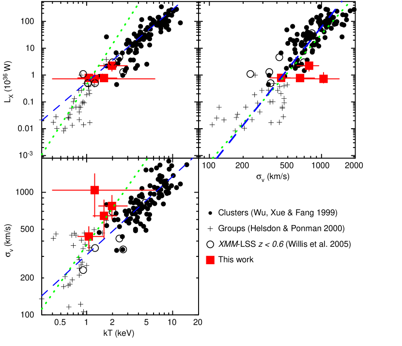
Figure 5: The correlation of global cluster properties: (top left) $L_{X}$–$T_{X}$ (bottom left) $T_{X}$–$\sigma_{v}$ (top right) $L_{X}$–$\sigma_{v}$. We compare our results with both rich clusters (Wu, Xue & Fang 1999) and poor groups (both the ‘loose’ and ‘compact’ sample from Helsdon & Ponman 2000), as well as more recent results from the XMM-Large Scale Structure (XMM-LSS) survey (Willis et al. 2005). In all parameter spaces shown, the sample in this work occupy the intermediate space between the rich/poor sample and are similar to the XMM-LSS sample. The dotted lines are the relationships derived for the groups sample from Helsdon & Ponman (2000), and the dashed lines show the equivalent relations derived using the rich cluster data from (Wu, Xue & Fang 1999). For clarity, we do not plot errors on the literature points (but these are taken into account in the linear fits). The X-ray data from this work are corrected for aperture losses. To estimate this, we extrapolate a King surface brightness profile of the form: $S(r)=S_{0}[1+({r}/{r_{\rm core}})^{2}]^{-3\beta+0.5}$. Assuming $\beta=0.5$ and $r_{\rm core}=200$ kpc, we find that the apertures used recover $\sim$80% of the total flux, extrapolating to $2r_{\rm core}$. All points are corrected to our adopted cosmology, with $H_{0}=75$ km s^-1 Mpc^-1.

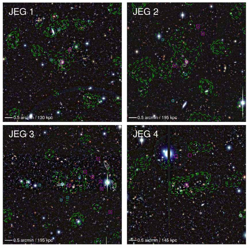
Figure 6: Here we present true colour image constructed from Subaru $BVi$-band $8^{\prime}\times 8^{\prime}$ images centered on the target radio galaxies JEG 1–4 (orientated North up and East left). In addition to the colour information, we overplot as contours the radio galaxy morphology from the VLA images (white solid), and X-ray (0.3–10 keV) contours (green dashed). The radio contour levels have been chosen to emphasise the lobe morphology (note that these are VLA B-array maps with a beam size of $5^{\prime}\times 4^{\prime\prime}$ with ${\rm P.A.}=170^{\circ}$, see S06), and the X-ray contours are slightly smoothed with a Gaussian kernel of width $\sim$$1^{\prime}$ and at $\sim$2,3,5 & 7$\sigma$ above the background in the vicinity of the environment. Finally, using the redshift data, we highlight galaxies which have $|\Delta v|<2000$ km s^-1 relative to the cluster redshift. We plot positive values of $\Delta v$ as open circles and negative values as open squares.

3.4 X-ray spectral fitting

The X-ray spectral fitting package xspec was used to fit X-ray spectral models to the cluster spectra. In terms of X-rays from galaxy clusters, it is commonly believed that the emission is predominantly due to the hot cluster gas trapped in the potential well, absorbed by the hydrogen column density within our own Galaxy (i.e. little in the way of internal cluster absorption is expected). The spectra therefore were fitted with a standard model comprised of a mekal hot plasma emission spectrum, together with a wabs photo-electric absorption model (Morrison & McCammon 1983). Due to the small number of counts, the hydrogen column of the absorption was fixed at the Galactic hydrogen column density in the line of sight to the Subaru pointings: $N_{\rm H}=2.55\times 10^{20}$ atoms cm^-2 (Dickey & Lockman 1990). Also the redshifts were fixed at the values given in Table 4. The temperature and metallicity were left free to optimize. Acceptable spectral fits were found for all the clusters (though only a small number of counts is seen from JEG 2), and these results are given in Table 4. We present the best fit gas temperature and metallicity (with respect to the Solar value), the errors being 90% for a single interesting parameter, and the (0.3$-$10 keV) absorption-corrected X-ray luminosity. Also tabulated are the best fit $\chi^{2}$ values and the number of degrees of freedom. For none of the clusters were there sufficient counts to warrant the use of a more complex model. We attempted to rebin the spectra into five counts per bin, with a fit based on Cash statistics (i.e. not subtracting the background in order to maintain counting statistics, Cash 1979), however this does not provide stronger constraints on $T$ or $Z$ compared to the adopted method. The data and best-fit models are shown in Figure 4.

4 Discussion

With the exception of JEG 2, the radio galaxies in each of our fields have environmental properties consistent with moderately rich groups at $z\sim 0.5$, in terms of their density statistic and X-ray properties. Despite the presence of a clear red sequence in the field of JEG 2 (Fig. 1), a simple $N_{0.5}$ environmental measure suggests that the environment is consistent with the field. However, it is likely that this is in fact a cluster of similar richness to JEG 1, JEG 3 and JEG 4 given that there are several nearby galaxies with colours and spectroscopic redshifts close to the radio galaxy. The low-number statistics for this system makes it difficult to make any robust comments about the radio-galaxy environment, except that this is probably a dynamically young group. There is some evidence for a sheet at $z\sim 0.65$ (Simpson et al. in prep) and JEG 2 may simply lie in an overdensity within this stucture. A large projected distribution of red galaxies around this group would in part explain the failure of the $B_{\rm gc}$ statistic to detect an overdensity: it could be possible that the control aperture itself is contaminated by the larger stucture.

Our observations of JEG 1 and JEG 4 also do not contain enough confirmed spectroscopic members at the radio galaxies’ redshifts to comment on their environments from a spectroscopic standpoint. The wide-angle radio tail of JEG 1 suggests rapid movement through a dense medium (S06), consistent with a group-group merger (e.g. Jetha et al. 2006). There is insufficient spectroscopic data to confirm this though. Furthermore, in the case of JEG 4, our results could be affected by a background group, although it is not clear that this is contributing significantly to the X-ray luminosity. This slightly more distant group could also be re-enforcing the strength of the red sequence (Fig. 1), and is a cautionary point regarding selection in this way.

4.1 Scaling relations

The X-ray luminosities derived by fitting thermal models to the X-ray spectra are remarkably constant over our radio galaxy sample, with the environment of JEG 3 the hottest and intrinsically the most luminous (we note that the small number of counts seen from JEG 2 results in a poorly constrained model). In Figure 5 we compare these clusters’ properties with the $L_{X}$–$T_{X}$ relation of Helsdon & Ponman’s (2000) study of galaxy groups and low-luminosity clusters, more luminous and massive systems from Wu, Xue & Fang (1999), as well as more intermediate redshift ($z<0.6$) X-ray selected groups/clusters from the XMM-Large Scale Survey (XMM-LSS; Willis et al. 2006).

Firstly, the four clusters all have high-$L_{X}$ and high-$T$ compared to the group sample, indicating that they bridge the gap between groups and rich clusters – a relatively unexplored region of parameter space. This is likely due to selection effects, thus there is potential in investigating these types of environment using a selection technique similar to the one outlined in this work. However, we note that the radio selected environments are quite similar to X-ray selected groups/clusters at similar redshifts, detected in the XMM-LSS (Willis et al. 2006). We show also the disparity between the slopes of the $L_{X}$–$T_{X}$ relation for groups (Helsdon & Ponman 2000) and rich clusters (Wu, Xue & Fang 1999), which differ by a factor $\sim$2. This is probably a real effect – the steepening of the slope for groups reflects the fact that these systems have a propsenity to exhibit deviations from the relation seen for the more massive systems due to processes other than cooling (Willis et al. 2005; Ponman, Cannon & Navarro 1999). Note that all the empirical relations found for groups and clusters are steeper than that expected for pure gravitational structure formation (Kaiser 1986); this implies that feedback as a source of energy input is important over all scales of clusters, but is more dominant in the low mass systems.

One can also compare the cluster X-ray luminosity and velocity dispersion with the $L_{X}$–$\sigma$ relations for these environments (Fig. 5). Although our small numer statistics provide only loose constraints on our environmental parameters, all our environments appear to have slightly large velocity dispersions compared to the temperature of the intracluster gas, although this is not statistically significant. Once again, the velocity dispersions and temperatures reveal that these radio galaxies inhabit intermediate environments between groups and clusters. A similar picture is revealed by the $L_{X}$–$\sigma_{v}$ relationship, with all clusters having slightly large $\sigma_{v}$ for their $L_{X}$. This is in good agreement with the observed velocity dispersions for other radio/optically selected samples (e.g. Rasumussen et al. 2006; Popesso et al. 2007).

For the remainder of the discussion we concentrate on JEG 3, which has a spectroscopically-confirmed sample large enough to comment on the Mpc-scale environment of the radio galaxy.

4.2 Discussion of JEG 3

Optically, the radio galaxy is intriguing: it appears to be morphologically disturbed, with a blue and red part, suggestive of a recent or ongoing interaction triggering star-formation. In fact, closer inspection of the spectra (and images) provide unambiguous evidence that the blue compenent is actually a strongly lensed background AGN or starburst galaxy at $z=1.847$ – not associated with the group (Figure 7). This high redshift object does not affect our results in any way, other than the fact that without the spectroscopic confirmation, this might be classified as a merger from the optical images alone. In terms of the radio emission, we are confident that the majority of the emission originates in the lensing source – i.e. the original selection of this target is still secure (the morphology and position of the radio emission support this, see Fig. 6). In terms of the impact from X-ray emission from the lensed galaxy, we also estimate that our measurements of the X-ray luminosity of the group will not be affected. The main bulk of the X-ray emission appears to be offset from the radio galaxy itself (Fig. 6) and the data were cleaned for point source emission prior to spectral fitting (§2.2). In the case that the point source is not cleaned, we estimate the impact on our measurement of $L_{X}$: if the lensed galaxy is a starburst, then we expect the X-ray luminosity to be of order $\sim 2\times 10^{34}$ W (based on an X-ray stack of $z\sim 2$ BM/BX galaxies, Reddy & Steidel 2004), although this will be boosted by the lens. If it is an AGN, then we might expect the X-ray luminosity to be higher by a factor $\sim$2 (Lehmer et al. 2005). In both cases, this has a negligible impact on our results.

The most obvious feature of JEG 3’s environment is the apparent spatial offset between the radio galaxy itself and the bulk of galaxies at the group redshift of 0.649 (Fig. 6), coincident with the dominant source of X-ray emission. The galaxy’s radio lobe morphology is suggestive of infall through a dense intracluster medium towards this higher density region. In Fig. 6 we represent the relative velocities of galaxies about the central redshift, indicating objects with $\pm\Delta v$. Note that there are two other radio galaxies in this group; one $\sim$$0.5^{\prime}$ to the west of the target radio galaxy, and the other (FR II source) several more arcminutes further to the west. Spectroscopic observations of these objects (Simpson et al. in prep) show that neither of them is associated with the structure surrounding JEG 3. These radio galaxies are not associated with the $z\sim 0.65$ structure identified around the radio galaxy in this work (see Simpson et al. in prep).

The radio galaxy appears to be associated with a small group interacting with the main body of the structure, thus it is not unreasonable to associate the triggering of the radio galaxy with this interaction. This is a scenario which has been seen in other radio galaxy environments, at both high and low redshifts, and over a wide range of radio powers (Simpson & Rawlings 2002). For example, the high redshift radio galaxy TN J1338$-$1942 ($z=4.1$, Venemans et al. 2003) belongs to a ‘proto-cluster’, but is offset from the centre of the overdensity. Similarly at low-redshift, the FR II source Cygnus A ($z=0.056$) is involved in an cluster-cluster merger (e.g. Ledlow et al. 2005), with the radio-source offset from the main overdensity (Owen et al. 1997). X-ray mapping of this cluster revealed hot (presumably) shocked gas between the two main peaks of the X-ray emission in the two sub-cluster units (Markevitch et al. 1999), consistent with the model of head-on cluster merging. These well studied radio galaxies are examples of the most luminous objects at their redshifts, whereas the luminosities of the radio galaxies in this work are modest in comparison. Triggering within interacting sub-cluster units seems to be responsible for a proportion of radio-galaxies, and this appears to have been happening at all epochs, and over a wide range of luminosities.

The triggering of the radio galaxy could have occurred via galaxy-galaxy interactions in its immediate group, while the X-ray emission seems to be centred on the richer group in which gas is plausibly being heated by gravitational processes. However, there is a further complication to the $L_{X}$–$T_{X}$ relationship, in that the outcome of the interaction between two sub-groups is a ‘boosting’ of the X-ray luminosity and temperature of the resulting cluster (Randall, Sarazin & Ricker 2002). In general this will temporarily (i.e. for a few 100 Myr) enhance both $L_{X}$ and $T_{X}$, before the cluster settles down to its equilibrium value. It is not clear what stage of interaction this environment is in. Given the relatively large offset between the X-ray emission and the radio galaxy, we postulate that this is in an early stage. In these environments it appears that we are witnessing radio galaxy activity and group-group merging/interaction at the same time. Although this may hint at radio galaxy triggering in the cluster assembly phase, this does not imply that all clusters containing a radio galaxy are in an unrelaxed state – most relaxed clusters also contain a central radio source. This is interesting in that it appears that radio galaxy activity can be important in the thermodynamic history of the cluster environment over a wide range of scales (i.e. groups to massive clusters) and various stages of development.

Following the assumption made in equation 4 of Miley (1980), and adopting an expansion speed of $0.03-0.15c$ (e.g. Scheuer 1995), we estimate the jet power of JEG 3 to be of the order 0.5–1$\times$10³⁶ W, which is comparable to the X-ray luminosity of the cluster (the expected contribution to the X-ray luminosity from the radio galaxy itself is not significant). Although the similarity in power is likely coincidental, it is interesting, because the radio output of this low-power source appears to be sufficient to balance the radiative cooling of the gas. However, it is unlikely that the radio galaxy could keep up this balance over a long period: this mechanical injection will end long before the main merger between the two groups stops imparting energy to the system, given the expected timescales of radio activity ($\lesssim$$10^{8}$ yr, Parma et al. 2002) which will likely be the dominant event in the pre-equilibrium thermodynamic history of the cluster. Nevertheless, since the radio-galaxy appears to have been triggered early in the life-time of the cluster (the centres of the radio and X-ray emission are separated by $\sim$200 kpc, Fig. 6), it could be important for providing significant energy input to the ICM, and therefore raising its entropy.

5 Summary

We have presented multi-object (Low Dispersion Survey Spectrograph 2) spectroscopy, combined with complimentary radio (VLA) and X-ray (XMM-Newton) observations of the Mpc-scale environments of a sample of low-power ($L_{1.4\,\rm GHz}\lesssim 10^{25}$ W Hz^-1) $z\sim 0.5$ galaxies in the Subaru-XMM Newton Deep Field (Simpson et al. 2004).

The radio galaxies targeted all appear to inhabit moderately rich groups, with remarkably similar X-ray properties, with JEG 3 (VLA 0033 in Simpson et al. 2006) being the hottest and residing in the richest environment. A statistical interpretation of the environment of JEG 2 (VLA 0011 in Simpson et al. 2006) would suggest that it does not belong to a cluster, but this could be in part due to the spatial distribution of the galaxies – the other evidence that this is a relatively rich group is compelling: there is a relatively strong red sequence and extended X-ray emission seen at this location (suggesting a gravitationally bound structure), and the spectroscopic data (although dominated by small number statistics) suggests that this is indeed a group, or part of a much larger structure, albeit one that is not relaxed. Also, three of the radio galaxies exhibit extended lobe morphology that suggest movement through a dense intracluster medium, again hinting that these systems are undergoing dynamical evolution.

Our analysis concentrates on the environment of JEG 3, which presents us with a ‘snap-shot’ of radio-galaxy and cluster evolution at $z\sim 0.65$. Overall, this is the richest environment we have studied, and the spectroscopic data reveal sub-structure: the radio galaxy belongs to a small group of galaxies which appears to be interacting (merging) with a larger group of galaxies. The X-ray emission for this system is associated with the richer, but radio-quiet group. We postulate that the radio emission has been triggered by a galaxy-galaxy merger within its local group. Although this may be providing some feedback to the ICM (indeed, the radio output is capable of balancing the overall radiative cooling), the eventual group-group interaction will boost the overall X-ray luminosity and temperature. This process will take longer than the life-time of the radio-source, and so might be the dominating event in the thermodynamic fate of the environment. This scenario is not dissimilar to the situation with other radio galaxies at both high redshift, and in the local Universe. Moreover, radio-triggering within sub-cluster units appears to be important for a proportion of the radio galaxy population over all epochs and luminosities.

6 acknowledgements

We thank an anonymous referee for helpful comments that greatly improved the clarity of this paper. We appreciate invaluable discussions with John Stott, Tim Beers, Alastair Edge and Mark Swinbank. The velocity code and data reduction software were kindly provided by Daniel Kelson. JEG, CS, SR & AR gratefully acknowledge support from the U.K. Science and Technology Facilities Council (formerly the Particle Physics and Astronomy Research Council).

References

- (1) Allen, S. W & Fabian, A., 1998, MNRAS, 297, L57
- (2) Allington-Smith, J. et al., 1994, PASP, 106, 983
- (3) Arnaud,& Evrard, 1999, MNRAS, 305, 631
- (4) Beers T., Flynn K., & Gebhardt K., 1990, AJ, 100, 32
- (5) Best, P., von der Linden, A., Kauffmann, G., Heckman, T. M., Kaiser, C. R., 2006, MNRAS, 368, L67
- (6) Bower, R. G., Benson, A. J., Malbon, R., Helly, J. C., Frenk, C. S., Baugh, C. M., Cole, S., Lacey, C. G., 2006, MNRAS, 370, 645
- (7) Cash, W., 1979, ApJ, 228, 939
- (8) Cole, S., et al., 2001, MNRAS, 326, 255
- (9) Croft R. A. C., Dalton G. B., Efstathiou G., 1999, MNRAS, 305, 547
- (10) Croton, D. J., et al., 2005, MNRAS, 356, 1155
- (11) Croton, D. J., et al., 2006, MNRAS, 636, 11
- (12) Cruz, et al. 2007, MNRAS, 375, 1349
- (13) David, L. P., Jones, C., Forman, W. 1995, Bulletin of the American Astronomical Society, 27, 1444
- (14) Dickey, J. M., Lockman, F. J., 1990, ARA&A, 28, 215
- (15) Edge, A. C., Stewart, C. G., 1991, MNRAS, 252, 414
- (16) Ellingson, E., Yee, H. K. C., Green, R. F., 1991, ApJ, 371, 49
- (17) Fanaroff, Riley, 1974, MNRAS, 167, 31
- (18) Farrah D., Geach, J., Fox, M., Serjeant, S., Oliver, S., Verma, A., Kaviani, A., Rowan-Robinson, M., 2004, MNRAS, 349, 518
- (19) Helsdon, S. F., Ponman, T. J., 2000, MNRAS, 319, 933
- (20) Hill G. J., & Lilly S. J., 1991, ApJ, 367, 1
- (21) Huang et al., 2003
- (22) Jarvis, M., et al., 2007, in prep
- (23) Jetha, N. N., Hardcastle, M. J. & Sakelliou, I., 2006, MNRAS, 368, 609
- (24) Kaiser, N., 1986, MNRAS, 222, 323
- (25) Kelson D. D., Illingworth, G. D., van Dokkum, P. G., Franx, M., 2000, ApJ, 531, 159
- (26) Kelson D. D. 2003, PASP, 115, 808
- (27) Kodama T. & Bower R.G., 2001, MNRAS, 321, 18
- (28) Kodama T., et al., 2004, MNRAS, 350, 1005
- (29) Ledlow, M. J., Owen, F. N., Miller, N. A., 2005, AJ, 130, 47L
- (30) Lehmer, B., et al., 2005, ApJ, 161, 21
- (31) Lilje P. B. & Efstathiou, G., 1988, MNRAS, 231, 635
- (32) Longair M. S. & Seldner, M., 1979, MNRAS, 189, 433
- (33) Lubin L., Oke B. & Postman M., 2002, AJ, 124, 1905
- (34) Markevitch, M., 1998, ApJ, 504, 27
- (35) Markevitch, M., Forman, W. R., Sarazin, C. L., Vikhlinin, A., 1999, ApJ, 521, 526
- (36) McLure, R. J., Willott, C. J., Jarvis, M. J., Rawlings, S., Hill, G. J., Mitchell, E., Dunlop, J. S., Wold, M., 2004, MNRAS, 351, 347
- (37) Miley, G., 1980, ARA&A, 18, 165
- (38) Moore B., Frenk C. S., Efstathiou G., Saunders W., 1994, MNRAS, 269, 742
- (39) Morrison, R. & McCammon, D., 1983, ApJ, 270, 119
- (40) Nevalainen, J. Markevitch, M. Lumb, D., 2005, ApJ, 629, 172
- (41) Norberg, P., et al., 2002, MNRAS, 332, 827
- (42) Owen, F. N., Ledlow, M. J., Morrison, G. E., Hill, J. M., 1997, ApJ, 488, L150
- (43) Parma, P., Murgia, M., de Ruiter, H. R. & Fanti, R., 2002, New Astronomy Reviews, 46, 313
- (44) Ponman, T. J. Cannon, D. B., Navarro, J. F., 1999, Nature, 397, 135
- (45) Popesso, P., Biviano, A., Böhringer, H., Romaniello, M., 2007, å, 461, 397
- (46) Randall, S. W., Sarazin, C. L. & Ricker, P. M., 2002, ApJ, 577, 579.
- (47) Rasmussen, J.; Ponman, T. J.; Mulchaey, J. S.; Miles, T. A.; Raychaudhury, S., 2006, MNRAS, 373, 653
- (48) Rawlings, S. & Saunders., Z, 1991, Nature, 349, 138
- (49) Rawlings, S. & Jarvis, M. J., 2004, MNRAS, 355, L9
- (50) Reddy, N. & Steidel, C. C., 2004, ApJ, 206, L13
- (51) Sekiguchi, S. & Ouchi, M., 2006, IAUS, 235, 359
- (52) Scheuer, P. A. G., 1995, MNRAS, 277, 331
- (53) Sijacki, D. & Springel, V., 2006, MNRAS, 366, 397
- (54) Simpson, C. & Rawlings, S., 2002, MNRAS, 334, 511
- (55) Simpson, C., et al., 2006, (S06), MNRAS, 372, 741
- (56) Springel, V., 2000, KITP Conference: Galaxy Formation and Evolution
- (57) Venemans, B. P., et al, 2002, ApJ, 569, L11
- (58) Venemans, B. P., Kurk, J. D., Miley, G. K., Rottgering, H. J. A., 2003, New Astronomy Reviews, 47, 353
- (59) Willis, J. P., et al., 2005, AJ, 124, 1905
- (60) Willis, J. P., Pacaud, F. Pierre, M, 2006, astro-ph/0610800
- (61) Wold M., Lacy M., Lilje P. B., Serjeant S., 2000, MNRAS, 316, 267
- (62) Wold M., Lacy M., Lilje P. B., Serjeant S., 2001, MNRAS, 323, 231
- (63) Wu, X.-P., Xue, Y.-J., Fang, L.-Z., 1999, ApJ, 524, 22
- (64) Yamada T., et al., 2005, astro-ph/0508594
- (65) Yee H. K. C. & López-Cruz O., 1999, AJ, 117, 1985
- (66) Yee H. K. C. & Ellingson E., 2003, AJ, 585, 215