A new doubly discrete analogue of smoke ring flow and the real time simulation of fluid flow

Abstract.

Modelling incompressible ideal fluids as a finite collection of vortex filaments is important in physics (super-fluidity, models for the onset of turbulence) as well as for numerical algorithms used in computer graphics for the real time simulation of smoke. Here we introduce a time-discrete evolution equation for arbitrary closed polygons in 3-space that is a discretisation of the localised induction approximation of filament motion. This discretisation shares with its continuum limit the property that it is a completely integrable system. We apply this polygon evolution to a significant improvement of the numerical algorithms used in Computer Graphics.

1. Introduction

The motion of vortex filaments in an incompressible, inviscid fluid has aroused considerable interest in quite different areas:

Differential geometry. The limiting case of infinitely thin vortex filaments leads to an evolution equation for closed space curves $\gamma$,

$$\dot{\gamma}=\gamma^{\prime}\times\gamma^{\prime\prime}.$$ (1)

Equation (1) was discovered in the beginning of the 20th century by Levi-Civita and his student Da Rios [1] and is called the smoke ring flow or localised induction approximation. In 1972 Hasimoto [2] discovered that the smoke ring flow is in fact a completely integrable Hamiltonian system equivalent to the non-linear Schrödinger equation. See [3] for more details on the history of the smoke ring equation. Subsequently the smoke ring flow has been studied by differential geometers as a natural evolution equation for space curves [4, 5, 6, 7]. Also discrete versions of the smoke ring flow in the form of completely integrable evolution equations for polygons with fixed edge length have been developed [8, 9, 10].

Fluid dynamics. As will be explained below, for applications in fluid mechanics a finite thickness of the vortex filaments has to be taken into account. The transition from infinitely thin filaments to filaments of finite thickness involves the incorporation of long range interactions (governed by the Biot-Savart law) between different filaments and different parts of the same filament into the purely local evolution equation (1). The resulting evolution of vortex filaments has been extensively studied both numerically and in the context of explaining the onset of turbulence [11]. Including in addition a small amount of viscosity in the equations leads to striking physical effects like vortex reconnection [12, 13, 14] and numerical techniques like “hairpin removal” [15, 16].

Computer graphics. Filament-based methods for fluid simulation are becoming important in Computer Graphics for special effects in motion pictures and for real time applications like computer games [17, 18]. Here the emphasis is on physical correctness and speed rather than numerical accuracy. Filament methods are ideal for these applications because complicated fluid motions can be created by a graphics designer by modelling the initial positions and strengths of the filaments. Moreover, filament methods work in unbounded space rather than in a bounded box (as is the case for grid-based methods [19]). This is desirable for the simulation of smoke.

The main goal of this paper is to improve the numerical algorithms currently used in Computer Graphics by applying the recent knowledge from Discrete Differential Geometry to the motion of polygonal smoke rings. Our method makes it possible to model thin filaments by polygons with arbitrarily few vertices. For comparison, using current methods to model a circular smoke ring which is thin enough to entrain smoke in a torus shape, it necessary to use a regular polygon with at least $800$ vertices.

In Section 2 we will explain the evolution equation for systems of vortex filaments that we will discretise. The resulting equations of motion are still Hamiltonian like the smoke ring flow (1). However, since already Poincaré knew that a system of vortex filaments consisting of more than three parallel straight lines (the “$n$-vortex problem”) fails to be an integrable system [20, p. 58f], we do not believe that this system is an integrable Hamiltonian system. Nevertheless it is a small perturbation of the integrable system constituted by the limit of infinitely thin filaments. This might be interesting for future investigations along the lines of KAM theory.

In Section 3 we consider polygonal vortex filaments. In this case, there is an elementary formula (11) for the Biot-Savart integral.

In Section 4 we will develop an extension of the known discrete-time smoke ring flow for polygons of constant edge lengths to arbitrary polygons. This is needed because after including the long range Biot-Savart interactions, the lengths of the edges will be no longer constant in time.

In the theory of integrable systems it is known at least since the 1980s that integrable difference equations may be interpreted as Darboux transformations of integrable differential equations [21, 22, 23]. In the meantime, this seminal discovery has lead to a reversed point of view, where the discrete integrable systems are considered fundamental and the continuous systems appear as smooth limits (see for example [24] and the references therein). In this vein, we will in Section 4 define the discrete-time integrable system in terms of iterated Darboux transformations of polygons and show afterwards that the smoke ring flow is obtained as a smooth limit.

In Section 5 we will describe our numerical method that very efficiently models the motion of fluids near the smoke ring limit.

2. Euler’s Equation for Vortex Filaments

Consider an incompressible, inviscid fluid in euclidean 3-space whose velocity field $u$ vanishes at infinity and whose vorticity $\omega=\mathop{\mathrm{curl}}\nolimits u$ is compactly supported. Then $u$ can be reconstructed from $\omega$ by the Biot-Savart formula

$$u(x)=-\frac{1}{4\pi}\int_{\mathbb{R}^{3}}\frac{x-z}{\left\|x-z\right\|^{3}}\times\omega(z)\,dz.$$ (2)

The equation of motion can then be written as

$$\dot{\omega}=[\omega,u].$$ (3)

Viewed as an evolution equation on the vector space $\mathcal{M}$ of compactly supported divergence-free vector fields on $\mathbb{R}^{3}$ this is a Hamiltonian system: A symplectic form $\sigma$ on $\mathcal{M}$ is defined as follows. Let $\omega\in\mathcal{M}$ and $\dot{\omega},\mathop{\hbox{}\omega}\limits^{\circ}\in T_{\omega}\mathcal{M}$. Then

$$\sigma_{\omega}(\dot{\omega},\mathop{\hbox{}\omega}\limits^{\circ})=\int_{\mathbb{R}^{3}}\det(\omega,\dot{\omega},\mathop{\hbox{}\omega}\limits^{\circ}).$$ (4)

Let $H:\mathcal{M}\rightarrow\mathbb{R}$ be the quadratic function

$$H=\int\!\!\!\int\frac{\langle\omega(x),\omega(y)\rangle}{\left\|x-y\right\|}\,dx\,dy,$$ (5)

where $\langle\cdot,\cdot\rangle$ is the euclidean scalar product on $\mathbb{R}^{3}$. Then $H$ is the Hamiltonian for the dynamical system (3). See [20, 25] for more details on this Hamiltonian description of ideal fluids.

If the vorticity of a fluid is concentrated on a closed curve $\gamma$ in a delta-function like manner, by Equation (2) the resulting velocity field $u$ becomes

$$u(x)=-\frac{\Gamma}{4\pi}\oint\frac{x-\gamma(s)}{\|x-\gamma(s)\|^{3}}\times\gamma^{\prime}(s)\,ds.$$ (6)

Here $\Gamma$ is the circulation around the filament. The problem with Equation (6) is that in order to determine the motion of $\gamma$ itself, $u$ has to be evaluated on $\gamma$, which results in a logarithmically divergent integral. Usually, this problem is handled by considering a vorticity field concentrated in a tube around $\gamma$ of small but finite radius $r$. For small $r$ the velocity in this tube is dominated by a term proportional to the localised induction approximation. (See, for example, [26, p. 36f].) Here we want to derive the smoke ring flow by taking the limit $r\rightarrow 0$. In order to prevent vortex filaments acquiring infinite speed, one has to scale the circulation $\Gamma$ down to zero when performing the limit to infinitely thin filaments. This means that the fluid velocity (6) goes to zero as well.

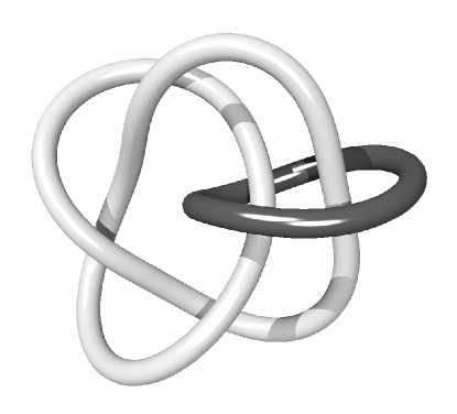
Figure 1. The space of links as the phase space for vortex filaments.

The resulting picture is then as follows: The fluid is completely at rest away from the filaments while the filaments just cut through the fluid with finite speed according to the smoke ring flow:

$$\dot{\gamma}_{j}=K_{j}\,\gamma_{j}^{\prime}\times\gamma_{j}^{\prime\prime}.$$ (7)

Here the constants $K_{j}$ account for the fact that the circulation of the different filaments $\gamma_{j}$ might go to zero at a different rate.

Equation (7) can be viewed as a completely integrable Hamiltonian system on the space of weighted links (see Figure 1) endowed with the symplectic form

$$\sigma_{\gamma}(\dot{\gamma},\mathop{\hbox{}\gamma}\limits^{\circ})=\sum_{j}K_{j}\oint_{\gamma_{j}}\det(\gamma_{j}^{\prime},\dot{\gamma},\mathop{\hbox{}\gamma}\limits^{\circ}).$$ (8)

For single curves this symplectic form is due to V. I. Arnold [20]. The corresponding Hamiltonian is a weighted sum of the filament lengths

$$H=\sum_{j}K_{j}\ \mathrm{Length}(\gamma_{j}).$$

Equation (7) can be obtained (using a simple renormalisation of time) as a limit as $a\rightarrow 0$ of the following system: Stick with (8) as the symplectic form, with $K_{j}$ replaced by the non-zero circulation $\Gamma_{j}$ around $\gamma_{j}$. As a Hamiltonian, use

$$H=\sum_{i,j}\frac{\Gamma_{i}\Gamma_{j}}{8\pi}\oint\!\!\oint\frac{\langle\gamma_{i}^{\prime}(s),\gamma_{j}^{\prime}(\tilde{s})\rangle}{\sqrt{a^{2}+\left\|\gamma_{i}(s)-\gamma_{j}(\tilde{s})\right\|^{2}}}\,ds\,d\tilde{s}.$$

The resulting equation of motion is

$$\dot{\gamma}_{i}(s)=-\sum_{j}\frac{\Gamma_{j}}{4\pi}\oint\frac{\gamma_{i}(s)-\gamma_{j}(\tilde{s})}{\sqrt{a^{2}+|\gamma_{i}(s)-\gamma_{j}(\tilde{s})|^{2}}^{\,3}}\times\gamma_{j}^{\prime}(\tilde{s})\,d\tilde{s}.$$ (9)

This equation of motion (9) can also be derived as follows:

• Smooth the delta-function like vorticity field $\omega_{0}$ of the link by a suitable convolution kernel and obtain

  $$\omega(x)=\frac{3a^{2}}{4\pi}\int_{\mathbb{R}^{3}}\frac{\omega_{0}(y)}{\sqrt{a^{2}+|x-y|^{2}}^{\,5}}\,dy.$$

• Compute the corresponding velocity field $u$ with $\mathop{\mathrm{curl}}\nolimits u=\omega$:

  $$u(x)=-\frac{\Gamma}{4\pi}\sum_{j}\oint\frac{x-\gamma_{j}(s)}{\sqrt{a^{2}+|x-\gamma_{j}(s)|^{2}}^{\,3}}\times\gamma_{j}^{\prime}(s)\,ds.$$ (10)

• Evaluate $u$ on the filaments to obtain (9).

To summarise: We model fluid motion near the filament limit by a Hamiltonian system on the space of weighted links. This system is still Hamiltonian but no longer integrable. Nevertheless it still has all the constants of motion induced by invariance with respect to the euclidean symmetry group. For example the weighted sum of the area vectors

$$A=\sum_{j}\Gamma_{j}\oint\gamma_{j}^{\prime}\times\gamma_{j}$$

is one of the preserved quantities. (Compare Theorem 4 of Section 4.)

The physical approximation implicit in our model is that we ignore possible deformations of the internal structure of the filaments and reduce everything to the evolution of the filament curves. The finite thickness of the filaments is taken into account by applying a fixed convolution kernel.

3. Polygonal Vortex Filaments

In order to develop a numerical method for modelling fluid motion near the filament limit we have to discretise the vortex filaments, i.e. we replace them by polygons. If $\gamma$ is a piecewise linear parametrisation of a closed polygon, on each edge we have $\gamma^{\prime\prime}=0$ and we find an explicit anti-derivative for the integrands of equation (10):

$$\Bigg{(}\frac{\langle\gamma,\gamma^{\prime}\rangle}{\sqrt{a^{2}+|\gamma|^{2}}\,\,(|\gamma^{\prime}|^{2}a^{2}+|\gamma\times\gamma^{\prime}|^{2})}\gamma\times\gamma^{\prime}\Bigg{)}^{\prime}=\frac{\gamma\times\gamma^{\prime}}{\sqrt{a^{2}+|\gamma|^{2}}^{\,3}}.$$ (11)

Here we have abbreviated $x-\gamma_{j}(s)$ to $\gamma$, $\gamma_{j}^{\prime}(s)$ to $\gamma^{\prime}$ and the prime is derivation with respect to $s$.

Inspection of Equation (11) reveals the following problem: The two adjacent edges have no influence at all on the velocity of a vertex. This amounts to effectively employing a distance cut-off in order to regularise the singular integral (6) for points on $\gamma$. It is known [26] that this is roughly equivalent to modelling vortex tubes of thickness equal to the edge length of the polygon. Using this model we would therefore be unable to model thin (and therefore fast) filaments without using excessively many edges for each polygon.

The contribution of local effects behaves like the smoke ring flow and the resulting equation of motion for a vertex $\gamma_{i}$ of a polygonal vortex filament $\gamma$ is then

$$\dot{\gamma}_{i}=u(\gamma_{i})+\lambda\kappa_{i}b_{i},$$ (12)

where $u$ is given by Equation (10) using (11), $\kappa_{i}b_{i}$ denotes curvature times binormal at $\gamma_{i}$, and $\lambda$ is constant for fixed $a$. Since the non-local effects quickly destroy any arc-length parametrisation (i.e. the lengths of the different edges of the polygon) and we do not have an adequate notion of curvature for arbitrary polygons, we can not evaluate (12) directly.

On the other hand, for polygons with constant edge lengths it is known that the doubly discrete smoke ring (or Hasimoto) flow [9] captures excellently the qualitative behaviour of the smooth smoke ring flow. In the next section we will discuss a version of this doubly discrete smoke ring flow which works also for polygons with varying edge lengths.

4. Darboux Transformation of Polygons

In this section we develop a discrete-time evolution for closed polygons that has the smoke ring flow (1) as a limit when the polygon approaches a smooth curve and the time-step goes to zero. This evolution (obtained by iterating so-called Darboux transformations) shares with its continuum limit the property that it is a completely integrable system in the sense that it comes from a Lax pair of quaternionic $2\times 2$-matrices with a spectral parameter. (This system therefore fits into the framework of [27].) The constants of the motion of the discrete system converge to constants of the motion of the smooth system in the limit.

Let $\gamma:\mathbb{Z}\rightarrow\mathbb{R}^{3}$ be an immersed polygon in $\mathbb{R}^{3}$, where immersed means that $\gamma_{i}\neq\gamma_{i+1}$ for all $i\in\mathbb{Z}$, and let $S_{i}=\gamma_{i+1}-\gamma_{i}$. If $\gamma$ is periodic with some period $n$, then the polygon is closed and $\gamma$ may be interpreted as a function on $\mathbb{Z}/n\mathbb{Z}$. In the following, we identify $\mathbb{R}^{3}$ with the imaginary quaternions $\mathrm{Im}\,\mathbb{H}=\{xi+yj+zk\,|\,x,y,z\in\mathbb{R}\}$.

Definition.

A polygon $\eta$ is called a Darboux transform of $\gamma$ with twist parameter $r\in\mathbb{R}$ and distance $l>0$, if $\|\eta_{i}-\gamma_{i}\|=l$ for all $i\in\mathbb{Z}$, and the normalised difference vectors $T_{i}$ defined by $lT_{i}=\eta_{i}-\gamma_{i}$ satisfy the quaternionic equation

$$T_{i+1}=(-r+lT_{i}-S_{i})T_{i}(-r+lT_{i}-S_{i})^{-1}.$$ (13)

The Darboux transformation of polygons and its relationship with the nonlinear Schrödinger equation and smoke ring flow was treated in [9] under the assumption that the polygon $\gamma$ has constant edge length. To drop this assumption was suggested to us by Tim Hoffmann [28].

Geometrically, Equation (13) has the following meaning (see Figure 2).

Figure 2. A polygon $\gamma$ and an edge of its Darboux transform $\eta$.

The difference vector $T_{i+1}$ is obtained from $T_{i}$ by a rotation with axis $lT_{i}-S_{i}$. The quadrilateral $\gamma_{i}\gamma_{i+1}\eta_{i+1}\eta_{i}$ is therefore a “folded parallelogram”. In particular, corresponding edges of $\gamma$ and $\eta$ have the same length. The angle of rotation is $2\arctan({\|lT_{i}-S_{i}\|}/{r})$. For $r=0$ it is $\pi$. For $r\rightarrow\pm\infty$, it goes to zero and in the limit the Darboux transformation becomes a translation.

Equation (13) can be written in the form

$$T_{i+1}=(aT_{i}+b)(cT_{i}+d)^{-1},$$ (14)

where $a,b,c,d\in\mathbb{H}$ depend on $S_{i}$ and the parameters $l,r$. That is, for each $i\in\mathbb{Z}$, $T_{i+1}$ is obtained by applying a quaternionic fractional linear transformation $f_{i}:\bar{\mathbb{H}}\rightarrow\bar{\mathbb{H}}$ to $T_{i}$, where $\bar{\mathbb{H}}=\mathbb{H}\cup\{\infty\}$. Indeed, (13) is equivalent to

$$T_{i+1}=\big{(}lT_{i}-r-S_{i}\big{)}\big{(}(r+S_{i})T_{i}+l\big{)}^{-1}.$$ (15)

To see this note that $T_{i}^{-1}=-T_{i}$ because $T_{i}$ is a purely imaginary unit quaternion, and hence $T_{i}(-r+lT_{i}-S_{i})^{-1}=(rT_{i}+l+S_{i}T_{i})$.

It is convenient to rewrite fractional linear transformations as matrix multiplication. Just as the extended complex plane $\bar{\mathbb{C}}=\mathbb{C}\cup\{\infty\}$ can be identified with the Riemann sphere $S^{2}$ and with the complex projective line $\mathbb{C}\mathrm{P}^{1}$, $\bar{\mathbb{H}}\cong S^{4}\cong\mathbb{H}\mathrm{P}^{1}$. The quaternionic projective line $\mathbb{H}\mathrm{P}^{1}$ is the set of (quaternionic) $1$-dimensional subspaces of the vector space $\mathbb{H}^{2}$ over $\mathbb{H}$. We consider $\mathbb{H}^{2}$ as right vector space: the product of a vector $\big{(}{p\atop q}\big{)}\in\mathbb{H}^{2}$ and a scalar $\lambda\in\mathbb{H}$ is $\big{(}{p\atop q}\big{)}\lambda=({p\lambda\atop q\lambda})$. A point

$$\Bigg{[}{p\atop q}\Bigg{]}=\Bigg{(}{p\atop q}\Bigg{)}\mathbb{H}\in\mathbb{H}\mathrm{P}^{1}$$

corresponds to the point $pq^{-1}\in\bar{\mathbb{H}}$, and $p,q$ are quaternionic homogeneous coordinates for this point. Now any fractional linear transformation of $\bar{\mathbb{H}}$ can be written as quaternionic $2\times 2$-matrix acting from the left on quaternionic homogeneous coordinates of $\mathbb{H}\mathrm{P}^{1}$: Writing $T_{i}$ in quaternionic homogeneous coordinates,

$$T_{i}=T^{(1)}_{i}(T^{(2)}_{i})^{-1},$$

one obtains from (15)

$$\left(\begin{array}[]{c}T^{(1)}_{i+1}\\ T^{(2)}_{i+1}\end{array}\right)=U_{i}(l,r)\left(\begin{array}[]{c}T^{(1)}_{i}\\ T^{(2)}_{i}\end{array}\right),\quad U_{i}(\lambda,\rho):=\left(\begin{array}[]{cc}\lambda&-\rho-S_{i}\\ \rho+S_{i}&\lambda\end{array}\right).$$ (16)

The following Theorem 1 characterises the Darboux transformations of polygons via a Lax pair of quaternionic $2\times 2$-matrices with spectral parameter. Theorem 2 is a permutability theorem for these Darboux transformations.

Theorem 1 (Lax pair).

Let $S_{i}=\gamma_{i+1}-\gamma_{i}$, $|T_{i}|=1$, and let $U_{i}(\lambda,\rho)$ be defined by (16) and

$$\tilde{U}_{i}(\lambda,\rho)=\left(\begin{array}[]{cc}\lambda&-\rho-\tilde{S}_{i}\\ \rho+\tilde{S}_{i}&\lambda\end{array}\right),$$

$$V_{i}(\lambda,\rho)=\left(\begin{array}[]{cc}\lambda&-\rho+r-lT_{i}\\ \rho-r+lT_{i}&\lambda\end{array}\right).$$

Then

$$V_{i+1}(\lambda,\rho)U_{i}(\lambda,\rho)=\tilde{U}_{i}(\lambda,\rho)V_{i}(\lambda,\rho)$$ (17)

for all $\lambda,\rho\in\mathbb{R}$, if and only if $S$ and $T$ satisfy (13) and

$$lT_{i+1}+S_{i}=\tilde{S}_{i}+lT_{i}.$$ (18)

That is, if and only if $\eta=\gamma+lT$ is a Darboux transform of $\gamma$ with twist parameter $r$ and distance $l$, and $\tilde{S}_{i}=\eta_{i+1}-\eta_{i}$.

Of course (17) means that the following diagram commutes:

$$\begin{array}[]{ccc}\mathbb{H}^{2}&\stackrel{{\scriptstyle\mbox{$\tilde{U}_{i}$}}}{{\longrightarrow}}&\mathbb{H}^{2}\\ \makebox[0.0pt][r]{$V_{i}$}\Big{\uparrow}&&\Big{\uparrow}\makebox[0.0pt][l]{$V_{i+1}$}\\ \mathbb{H}^{2}&\stackrel{{\scriptstyle\mbox{$U_{i}$}}}{{\longrightarrow}}&\mathbb{H}^{2}\end{array}$$

Proof.

Note that in general for quaternionic $2\times 2$-matrices with $a_{+},a,b,\tilde{b}\in\mathbb{H}$ and $\lambda\in\mathbb{R}$ the equality

$$\left(\begin{array}[]{cc}\lambda&a_{+}\\ -a_{+}&\lambda\end{array}\right)\left(\begin{array}[]{cc}\lambda&b\\ -b&\lambda\end{array}\right)=\left(\begin{array}[]{cc}\lambda&\tilde{b}\\ -\tilde{b}&\lambda\end{array}\right)\left(\begin{array}[]{cc}\lambda&a\\ -a&\lambda\end{array}\right)$$

is equivalent to

$$a_{+}b=\tilde{b}a\qquad\textrm{and}\qquad\lambda(a_{+}+b)=\lambda(\tilde{b}+a).$$

It follows that (17) holds for all $\lambda\in\mathbb{R}$, if and only if (18) holds and

$$(-\rho+r-lT_{i+1})(-\rho-S_{i})=(-\rho-\tilde{S}_{i})(-\rho+r-lT_{i}).$$

Use (18) to eliminate $\tilde{S}_{i}$ from this equation and gather terms of equal power in $\rho$ on both sides. The coefficients of $\rho^{2}$ are both 1, and the coefficients of $\rho$ are obviously equal. What remains is the equation

$$(r-lT_{i+1})(-S_{i})=(-S_{i}-lT_{i+1}+lT_{i})(r-lT_{i}).$$

Solve for $T_{i+1}$ to obtain (13). ∎

Theorem 2 (Permutability).

Suppose $\eta=\gamma+lT$ is a Darboux transform of $\gamma$ with twist parameter $r$ and distance $l$, and $\hat{\eta}=\gamma+\lambda\hat{T}$ is a Darboux transform of $\gamma$ with twist parameter $\rho$ and distance $\lambda$, then $\eta+\lambda\tilde{T}$ with

$$\tilde{T}=\big{(}\lambda\hat{T}-\rho+r-lT\big{)}\big{(}(\rho-r+lT)\hat{T}+\lambda\big{)}^{-1}$$ (19)

is a Darboux transformation of $\eta$ with twist parameter $\rho$ and distance $\lambda$.

Proof.

Note that $\tilde{T}_{i}$ is obtained by applying the quaternionic fractional linear transformation represented by the matrix $V_{i}(\lambda,\rho)$ to $\hat{T}_{i}$. Let us write $\tilde{T}_{i}=V_{i}(\lambda,\rho)\hat{T}_{i}$ for short. Since $\hat{\eta}$ is a Darboux transform of $\gamma$ with twist parameter $\rho$ and distance $\lambda$, Equation (16) says that $\hat{T}_{i+1}=U_{i}(\lambda,\rho)\hat{T}_{i}$. Now Theorem 1 implies $\tilde{T}_{i+1}=\tilde{U}_{i}(\lambda,\rho)\tilde{T}_{i}$ and hence (again by Equation (16)), $\eta+\lambda\tilde{T}$ is a Darboux transformation of $\eta$ with twist parameter $\rho$ and distance $\lambda$. ∎

Even if $\gamma$ is a closed curve, the curves obtained by iterating (13) will in general not close up. However, we will see that any closed curve has generically two closed Darboux transforms.

The fractional linear transformations $f_{i}:T_{i}\mapsto T_{i+1}$ that are represented by the matrices $U_{i}(l,r)$ have the special property that they map the unit sphere $S^{2}=\{q\in\mathrm{Im}\,\mathbb{H}\,|\,q^{2}=-1\}$ to itself. This follows directly from (13). Hence the restrictions $f_{i}|_{S^{2}}$ are Möbius transformations of $S^{2}$. In fact, they are orientation preserving Möbius transformations: By continuity, it is enough to check this for a particular value of $r$ and $l$; and for $r=0$, $l=0$ one obtains $T_{i+1}=S_{i}T_{i}S_{i}^{-1}$, which is a $180^{\circ}$ rotation with axis $S_{i}$.

In order to find for given $l$, $r$ the closed Darboux transforms of $\gamma$, one has to look for choices of the initial unit vector $T_{0}$ such that the recursion (15) generates a sequence with period $n$, i.e. $T_{0}=T_{n}$. The composition $f_{n-1}\circ\ldots\circ f_{0}$, which maps $T_{0}\mapsto T_{n}$, is represented by the monodromy matrix

$$H_{l,r}=U_{n-1}(l,r)\cdots U_{2}(l,r)U_{1}(l,r)U_{0}(l,r).$$

It is is itself an orientation-preserving Möbius transformation of the unit sphere $S^{2}$ onto itself. For special cases (we will see below that this cannot happen for all $l$, $r$) this Möbius-transformation could be the identity, but in general it will have exactly two fixed points (counted with multiplicity).

With each closed curve $\gamma$ we have thus associated a monodromy map $f_{n-1}\circ\ldots\circ f_{0}$. $T_{0}$ will be a fixed point if and only if $\left(T_{0}\atop 1\right)$ is an eigenvector of the monodromy matrix $H_{l,r}$. The following theorem is an immediate consequence of Theorem 1.

Theorem 3.

Suppose $\eta=\gamma+lT$ is a closed Darboux transform of $\gamma$ with distance $l$ and twist parameter $r$. Then for all $\lambda$ and $\rho$, the monodromy matrix $H^{\eta}_{\lambda,\rho}$ of $\eta$ is conjugate to the monodromy matrix $H_{\lambda,\rho}$ of $\gamma$:

$$H^{\eta}_{\lambda,\rho}=V_{0}(\lambda,\rho)H_{\lambda,\rho}V_{0}(\lambda,\rho)^{-1}.$$ (20)

This means that if $\left(\hat{T}_{0}\atop 1\right)$ is an eigenvector of $H_{\lambda,\rho}$, then $V_{0}(\lambda,\rho)\left(\hat{T}_{0}\atop 1\right)$ is an eigenvector of $H^{\eta}_{\lambda,\rho}$.

Moreover, one can compute all closed Darboux transforms of $\eta$ without having to solve an eigenvalue problem, even without iterating the $f_{i}$. Indeed, by Theorem 2, all closed Darboux transforms of $\eta$ are given by (19).

Theorem 3 implies that apart from the edge lengths there are many other quantities connected with closed polygons that are invariant under Darboux transforms: For each $\lambda$, $\rho$ the conjugacy class of the monodromy matrix $H_{\lambda,\rho}$ is invariant. We will show that this implies a nice geometric invariant: The area vector of a closed polygon turns out to be invariant under Darboux transformations (Theorem 4).

To derive the invariance of the area vector from the invariance of the conjugacy class of the monodromy matrix, we equip the set of quaternionic $2\times 2$-matrices of the form

$$\left(\begin{array}[]{cc}a&-b\\ b&a\end{array}\right),\ \ a,b\in\mathbb{H}$$ (21)

with the structure of a $\mathbb{C}$-algebra that is isomorphic to $gl(2,\mathbb{C})$. First note that a quaternionic $2\times 2$-matrix is of the form (21) precisely if it commutes with

$$J=\left(\begin{array}[]{cc}0&-1\\ 1&0\end{array}\right).$$

Define the multiplication of such a matrix with a scalar $\lambda+i\rho\in\mathbb{C}$ by

$$(\lambda+i\rho)A=(\lambda I+\rho J)A,$$ (22)

where $I$ is the identity matrix.

The complex multiples of the identity are then

$$Z=(\lambda+i\rho)I=\lambda I+\rho J=\left(\begin{array}[]{cc}\lambda&-\rho\\ \rho&\lambda\end{array}\right).$$ (23)

Thus we can write $U_{i}(\lambda,\rho)$ and $V_{i}(\lambda,\rho)$ as

$$U_{i}(\lambda,\rho)=(\lambda+i\rho)I+J\left(\begin{array}[]{cc}S_{i}&0\\ 0&S_{i}\end{array}\right),$$

$$V_{i}(\lambda,\rho)=(\lambda+i\rho)I+J\left(\begin{array}[]{cc}-r+lT_{i}&0\\ 0&-r+lT_{i}\end{array}\right).$$

Remark.

This means we can combine $\lambda$ and $\rho$ into one complex spectral parameter $\lambda+i\rho$.

Equation (23) also implies that the trace-free complex matrices in $gl(2,\mathbb{C})$ correspond to those matrices of the form (21) with $a,b\in\mathrm{Im}\mathbb{H}$. Further, a matrix of the form (21) has $a,b\in\mathrm{Im}\mathbb{H}$ precisely if its square is a matrix of the form (23), that is, a (complex) multiple (with multiplication defied by (22)) of the identity. Identifying $\mathbb{C}$ with the matrices of the form (23) we obtain

$$\frac{1}{2}\mathop{\mathrm{tr}}\nolimits_{\mathbb{C}}\left(\begin{array}[]{cc}a&-b\\ b&a\end{array}\right)=\mathrm{Re}\,a+(\mathrm{Re}\,b)J$$

and

$$\det_{\mathbb{C}}\nolimits\left(\begin{array}[]{cc}a&-b\\ b&a\end{array}\right)=\frac{1}{2}((\mathop{\mathrm{tr}}\nolimits A)^{2}-\mathop{\mathrm{tr}}\nolimits A^{2})=|a^{2}|-|b^{2}|+2\langle a,b\rangle J.$$

In particular

$$\det_{\mathbb{C}}\nolimits\left(\begin{array}[]{cc}l&-r-S\\ r+S&l\end{array}\right)=l^{2}-r^{2}-|S|^{2}+2lrJ,$$

which vanishes precisely when $r=0,l=\pm|S|$. Using the notation

$$\mathit{diag}(S):=\left(\begin{array}[]{cc}S&0\\ 0&S\end{array}\right)$$

for $S\in\mathbb{H}$ we can express $H_{\lambda,\rho}$ as

$$H_{Z}=(Z+J\mathit{diag}(S_{n-1}))\cdots(Z+J\mathit{diag}(S_{0})),$$

with $Z$ given by (23). Hence $\det_{\mathbb{C}}\nolimits H_{Z}$ is a complex polynomial of degree $2n$ with zeroes precisely at $Z=\pm|S_{0}|$, …, $\pm|S_{n-1}|$. By Theorem 3 this determinant is invariant under Darboux transforms. This just corresponds to the fact that the edge lengths are invariant by construction. Non-trivial further invariants come from the complex polynomial

$$P(Z)=\mathop{\mathrm{tr}}\nolimits_{\mathbb{C}}H_{Z}$$

of degree $n$. Let us look at the polynomial coefficients of $H_{Z}$ itself:

$$H_{Z}=\sum_{k=1}^{n}Z^{k}A_{n-k},$$

where

$$A_{k}=J^{k}\sum_{n-1\geq j_{1},...,j_{k}\geq 0}\mathit{diag}({S}_{j_{1}}\cdots{S}_{j_{k}}).$$

In particular,

$$A_{0} =I,$$

$$A_{1} =J^{k}\sum_{k=0}^{n-1}\mathit{diag}({S}_{k})=0,$$

$$A_{2} =-\sum_{n-1\geq i>j\geq 0}\mathit{diag}({S}_{i}{S}_{j}).$$

That is, $A_{2}$ is a diagonal matrix with both diagonal entries equal to

$$q=-\sum_{n-1\geq i>j\geq 0}S_{i}S_{j}.$$

The real part of $q$ is

$$\mathrm{Re}(q) =\sum_{n-1\geq i>j\geq 0}\langle S_{i},S_{j}\rangle=\frac{1}{2}\sum_{i\neq j}\langle S_{i},S_{j}\rangle=\frac{1}{2}|\sum_{i=0}^{n-1}S_{i}|^{2}-\frac{1}{2}\sum_{i=0}^{n-1}|S_{i}|^{2}$$

$$=-\frac{1}{2}\sum_{i=0}^{n-1}|S_{i}|^{2}.$$

This is a function of the edge lengths and therefore not interesting. The imaginary part of $q$ is given by

$$2A:=\mathop{\mathrm{Im}}(q) =-\sum_{i>j}S_{i}\times S_{j}$$

$$=\sum_{j=1}^{n-1}\left(\sum_{i=1}^{n-1}S_{i}\right)\times S_{j}$$

$$=\sum_{j=1}^{n-1}(\gamma_{j}-\gamma_{0})\times(\gamma_{j+1}-\gamma_{j})$$

$$=\sum_{j=1}^{n-1}(\gamma_{j}-\gamma_{0})\times(\gamma_{j+1}-\gamma_{0}).$$

This invariant $A$ is just the area vector. The following proposition (with obvious proof) clarifies its geometrical meaning.

Proposition 1.

Let $a\in\mathbb{R}^{3}$ be a unit vector, $|a|=1$, and endow the plane $a^{\perp}$ with the volume form

$$\det_{a^{\perp}}\nolimits(X,Y):=\det_{\mathbb{R}^{3}}\nolimits(a,X,Y).$$

Then the area enclosed by the orthogonal projection $\hat{\gamma}$ of the polygon $\gamma$

$$\hat{\gamma}_{n}=\gamma_{n}-\langle\gamma_{n},a\rangle a$$

is equal to $\langle M,a\rangle$.

This explains the name area vector: It encodes all the projected areas.

Theorem 4.

The area vector $A$ is invariant under Darboux transforms.

Proof.

By (20), the monodromy matrix of the Darboux transformed curve $\eta$,

$$H^{\eta}_{Z}=\sum_{k=0}^{n}Z^{k}A^{\eta}_{n-k},$$

satisfies

$$H^{\eta}_{Z}(Z+J(-rI+l\,\mathit{diag}{T}_{0}))=(Z+J(-rI+l\,\mathit{diag}{T}_{0}))H_{Z}$$ (24)

Using

$$H_{Z} = Z^{n}+Z^{n-2}A_{2}+...+A_{0},$$

$$H^{\eta}_{Z} = Z^{n}+Z^{n-2}A^{\eta}_{2}+...+A_{0}^{\eta}$$

and comparing the $Z^{n-2}$-coefficients in both sides of (24) we obtain $A^{\eta}_{2}=A_{2}$. ∎

Finally we consider the continuum limit of smooth curves $\gamma:S^{1}\rightarrow\mathbb{R}^{3}$ and indicate why Darboux transforms with small parameters $l$, $r$ do indeed converge to the smoke ring flow (1). The continuum limit of (13) is obtained by replacing $S$ by $hS$ and then computing $T^{\prime}:=\frac{d}{dh}\big{|}_{h=0}T_{h}$. The resulting differential equation is

$$T^{\prime}=(TS-ST)(-r+lT)^{-1}$$

or

$$T^{\prime}=\frac{2}{r^{2}+l^{2}}T\times(lT\times S-rS),$$ (25)

where $S:\mathbb{R}\rightarrow\mathbb{R}^{3}$ is given by

$$\gamma^{\prime}=S.$$

One can check that, as expected, the transformed curve $\eta=\gamma+lT$ satisfies

$$|\eta^{\prime}|=|\gamma^{\prime}|.$$

The monodromy of the ODE (25) is a Möbius transformation of $S^{2}$ that generically has exactly two fixed points. Thus, for generic parameters $l$ and $r$ a space curve $\gamma$ has exactly two closed Darboux transforms.

Assume now that we have for $r=-l$ a family of such closed Darboux transforms $\eta_{l}$ that depend analytically on $l$. Then we reparametrise $\eta_{l}$ as

$$\gamma_{l}(s):=\eta_{l}(s-l)=\gamma(s-l)+lT_{l}(s-l).$$ (26)

Then $\gamma_{0}=\gamma$ and comparing coefficients of $l$ in the power series expansion of (26) we obtain

$$\frac{\partial}{\partial l}\,\Big{|}_{l=0}\,\gamma_{l}=0,\qquad\frac{\partial^{2}}{\partial l^{2}}\,\Big{|}_{l=0}\,\gamma_{l}=\gamma^{\prime}\times\gamma^{\prime\prime}.$$

Hence

$$\gamma_{l}-\gamma_{0}=l^{2}\gamma^{\prime}\times\gamma^{\prime\prime}+O(l^{3}).$$

A small time-step $\Delta t$ of the smoke ring flow is therefore approximated by a Darboux transform with length $l$ given by $l^{2}=\Delta t$.

Remark.

In order to eliminate the reparametrising effect of the Darboux transforms it is convenient to apply first a Darboux transform with parameters $l$ and $-r$ followed by a reverse Darboux transform with parameters $l$ and $r$. This will cancel out the (first order in $t$) tangential shift and leave only the (second order in $t$) smoke ring evolution (see [8]).

5. An algorithm for the real time simulation of fluid flow

Based on the theoretic foundations covered in the previous sections, we have implemented the following algorithm for the simulation of fluid flow. Our aim was to develop an algorithm which is fast enough to generate realistic looking computer animations of fluid motion in real time. Figure 3 shows a sample screen shot from a simulation which runs smoothly on standard hardware.

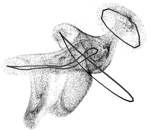
Figure 3. $256^{2}$ fluid particles evolving under the influence of three polygonal vortex filaments.

We assume the vorticity is concentrated along a few vortex rings, which we represent by closed polygons. Their motion is governed by a mixture of the velocity field induced by the polygonal vortex rings via the smoothed Biot-Savart formula (10) of Section 3, and Darboux transformations which approximate a time step of the polygonal smoke ring flow as explained in Section 4. The rationale behind this scheme is that the velocity field induced by an edge of a polygonal vortex filament is zero on that edge itself. Thus, the adjacent edges do not contribute to the velocity of a vertex. The Darboux transforms make up for this lack of local interaction. The following is a summary description of the algorithm. Details (in particular how we set the parameters $r_{i}$ and $l_{i}$ of the Darboux transformation) are given below.

• input:

  • positions $\gamma_{ij}$ of the $j$th vertex of the $i$th polygonal vortex filament $\gamma_{i}$, where $i=1\ldots m$, $j=1\ldots n_{i}$.

  • strengths $\Gamma_{i}$ and smoothing (thickness) parameters $a_{i}$ of the vortex filaments.

  • positions $p_{i}\in\mathbb{R}^{3}$ of advected particles, where $i=1\ldots k$.

  • time-step $\Delta t$ .

• loop:

  • Compute a double Darboux transform $\eta_{i}$ with parameters $\mp r_{i},l_{i}$ of each polygon $\gamma_{i}$. $\gamma_{ij}\leftarrow\eta_{ij}$.

  • Solve $\dot{\gamma}_{ij}=u(\gamma_{ij})$ for time-step $\Delta t$, where $u(x)$ is the velocity field obtained by the smoothed Biot-Savart formula (10).

  • Update the particle positions $p_{i}$ by solving $\dot{p}_{i}=u(p_{i})$ for time-step $\Delta t$.

In Step 1, we determine the parameters $l_{i}$ and $r_{i}$ as follows. The amount of smoke ring flow needed to make up for the lack of local interaction depends on the thickness $a_{i}$, the number of edges $n_{i}$ and the total length $L_{i}$ of $\gamma_{i}$. Since we do not know the correct speed for an arbitrary polygon, we determine the parameters for the test case of a regular $n_{i}$-gon with same strength, thickness and total length. We choose the parameters in such a way that for the regular $n_{i}$-gon the sum of self-induced velocity from the Biot-Savart formula (10) plus the effect of a double Darboux transform coincides with the analytically known speed $U_{i}$ for a circle with same length $L_{i}$:

$$U_{i}=\frac{\Gamma_{i}}{2L_{i}}\left(\ln\frac{4L_{i}}{\pi a_{i}}-1\right),$$ (27)

compare [26, p. 212]. We compute the self-induced speed $\tilde{U}_{i}$ of the $n_{i}$-gon by evaluating the smoothed Biot-Savart formula (10) at one vertex for all edges of the $n_{i}$-gon. This speed is slower than $U_{i}$ because the adjacent edges have no influence on a vertex, see Section 3. Now we choose $r_{i}$ and $l_{i}$ such that a double Darboux transformation translates the regular $n_{i}$-gon by a distance of $(U_{i}-\tilde{U}_{i})\,\Delta t$. A single Darboux transform of the regular $n_{i}$-gon is a translation in binormal direction plus a non-zero rotation about the centre axis. The rotation cancels out for a double Darboux transform and is therefore arbitrary. We choose the rotation angle to be $2\pi/n_{i}$, which leads to the following formulas for $l_{i}$ and $r_{i}$:

$$l_{i}=\sqrt{\left(L_{i}/n_{i}\right)^{2}+\sigma_{i}^{2}}\;,\qquad r_{i}=\sigma_{i}\cot(\pi/n_{i})\,,$$

where we have abbreviated $\frac{1}{2}(U_{i}-\tilde{U}_{i})\,\Delta t$ by $\sigma_{i}$.

In Step 2, we use the fourth order Runge-Kutta scheme (RK4) to solve the ordinary the differential equation $\dot{x}=u(x)$ for the time-step $\Delta t$. To advect the large number of particles in Step 3 we use second order Runge-Kutta (RK2), where we use the two polygon positions after Step 1 and Step 2 as intermediate values. To improve performance further, this step is computed on the computer’s graphics chip (GPGPU).

Evaluating $u(x)$ via Equation (10) is unproblematic, because the integral on the right hand side can be solved explicitly for straight line segments; see Equation (11) in Section 3.

References

- [1] L. Sante Da Rios. Sul moto d’un liquido indefinito con un filetto vorticoso di forma qualunque. Rendiconti del Circolo Matematico Palermo, 22:117–135, 1906.
- [2] H. Hasimoto. A soliton on a vortex filament. Journal of Fluid Mechanics, 51:477–485, 1972.
- [3] R. L. Ricca. Rediscovery of Da Rios Equations. Nature, 352:561–562, 1991.
- [4] A. Calini and T. Ivey. Finite-gap solutions of the vortex filament equation: Genus one solutions and symmetric solutions. J. Nonlinear Sci., 15(5):321–361, 2005.
- [5] J. Cieśliński, P. K. H. Gragert, and A. Sym. Exact solution to localized-induction-approximation equation modeling smoke ring motion. Phys. Rev. Lett., 57(13):1507 – 1510, 1986.
- [6] T. A. Ivey. Geometry and topology of finite-gap vortex filaments. In I. M. Mladenov and M. de León, editors, Geometry, Integrability, and Quantization. Proceedings of the 7th International Conference held in Varna June 2–10 2005, pages 187–202, Sofia, 2006.
- [7] J. Langer and R. Perline. The Hasimoto transformation and integrable flows on curves. Appl. Math. Lett, 3:61–64, 1990.
- [8] T. Hoffmann. Discrete curves and surfaces. PhD thesis, Technische Universität Berlin, 2000.
- [9] T. Hoffmann. Discrete Hashimoto surfaces and a doubly discrete smoke ring flow. In A. I. Bobenko, P. Schröder, J. M. Sullivan, and G. M. Ziegler, editors, Lectures on Discrete Differential Geometry, Oberwolfach Seminars. Birkhäuser, Basel, in preparation. Preprint arXiv:math/0007150v1.
- [10] A. Doliwa and P. M. Santini. Integrable dynamics of a discrete curve and the Ablowitz-Ladik hierarchy. J. Math. Phys., 36(3):1259–1273, 1995.
- [11] A. J. Chorin. Vorticity and Turbulence, volume 103 of Appl. Math. Sci. Ser. Springer, New York, 1991.
- [12] J. Koplik and H. Levine. Vortex reconnection in superfluid helium. Phys. Rev. Lett., 71(9):1375–1378, Aug 1993.
- [13] D. Kivotides and A. Leonard. Computational model of vortex reconnection. Europhys. Lett., 63:354–360, 2003.
- [14] P. Chatelain, D. Kivotides, and A. Leonard. Reconnection of colliding vortex rings. Phys. Rev. Lett., 90(5):054501, Feb 2003.
- [15] A. J. Chorin. Hairpin removal in vortex interactions. J. Comput. Phys., 91(1):1–21, 1990.
- [16] A. J. Chorin. Hairpin removal in vortex interactions II. J. Comput. Phys., 107(1):1–9, 1993.
- [17] A. Angelidis and F. Neyret. Simulation of smoke based on vortex filament primitives. In ACM-SIGGRAPH/EG Symposium on Computer Animation (SCA), 2005.
- [18] A. Angelidis, F. Neyret, K. Singh, and D. Nowrouzezahrai. A controllable, fast and stable basis for vortex based smoke simulation. In ACM-SIGGRAPH/EG Symposium on Computer Animation (SCA), sep 2006.
- [19] J. Stam. Stable fluids. In SIGGRAPH ’99: Proceedings of the 26th annual conference on Computer graphics and interactive techniques, pages 121–128, New York, NY, USA, 1999. ACM Press/Addison-Wesley Publishing Co.
- [20] V. A. Arnold and B. A. Khesin. Topological Methods in Hydrodynamics, volume 125 of Applied mathematical sciences. Springer, New York, 1998.
- [21] D. Levi and R. Benguria. Backlund transformations and nonlinear differential difference equations. Proc. Natl. Acad. Sci. USA, 77(9):5025–5027, 1980.
- [22] D. Levi. Nonlinear differential difference equations as Backlund transformations. J. Phys. A, 14(5):1083–1098, 1981.
- [23] F. W. Nijhoff, G. R. W. Quispel, and H. W. Capel. Direct linearization of nonlinear difference-difference equations. Phys. Lett. A, 97(4):125–128, 1983.
- [24] V. E. Adler, A. I. Bobenko, and Yu.B. Suris. Classification of integrable equations on quad-graphs. The consistency approach. Comm. Math. Phys., 233(3):513–543, 2003.
- [25] D. Ebin and J. Marsden. Groups of diffeomorphisms and the motion of an incompressible fluid. Ann. of Math., 92:102–163, 1970.
- [26] P. G. Saffman. Vortex Dynamics. Cambridge University Press, Cambridge, 1992.
- [27] A. I. Bobenko and Yu. B. Suris. Integrable noncommutative equations on quad-graphs. The consistency approach. Lett. Math. Phys., 61(3):241–254, 2002.
- [28] T. Hoffmann, 2005. Personal communication.