Abstract

We study efficient broadcasting for wireless sensor networks, with network coding. We address this issue for homogeneous sensor networks in the plane. Our results are based on a simple principle (IREN/IRON), which sets the same rate on most of the nodes (wireless links) of the network. With this rate selection, we give a value of the maximum achievable broadcast rate of the source: our central result is a proof of the value of the min-cut for such networks, viewed as hypergraphs. Our metric for efficiency is the number of transmissions necessary to transmit one packet from the source to every destination: we show that IREN/IRON achieves near optimality for large networks; that is, asymptotically, nearly every transmission brings new information from the source to the receiver. As a consequence, network coding asymptotically outperforms any scheme that does not use network coding.

Near Optimal Broadcast
 with Network Coding
 in Large Sensor Networks

Introduction

Seminal work in [1] has introduced the idea of network coding, whereby intermediate nodes are mixing information from different flows (different bits or different packets).

One logical domain of application is wireless sensor networks. Indeed, for wireless networks, a generalization of the results in [1] exists: when the capacity of the links are known and fixed, the maximal broadcast rate of the source can be computed, as shown in [3]. Essentially, for one source, it is the min-cut of the network from the source to the destinations, as for wired networks [1], but considering hypergraphs rather than graphs. This is true whether the rate and the capacity are expressed in bits per second or packets per second [4].

However, in wireless sensor networks, a primary constraint is not necessarily the capacity of the wireless links: because of the limited battery of each node, the limiting factor is the cost of wireless transmissions. Hence a different focus is energy-efficiency, rather than the maximum achievable broadcast rate:

$\bullet$ Given one source, minimize the total number of transmissions used to achieve the broadcast to destination nodes.

The problem is no longer related to the capacity, because the same transmissions can be streched in time, with an identical cost. However, one can still imagine using network coding, where each node repeats combinations of packets with an average interval between transmissions: this defines the rate of the node, and the rate is an unknown.

The problem of energy-efficiency is to compute a set of transmission rates for each node, with minimal cost. With network coding, the problem turns out to be solvable in polynomial time: for the stated problem, [5, 6] describe methods to find the optimal transmission rate of each node with a linear program. However, this does not necessarily provide direct insight about the optimal rates and their associated optimal cost: those are obtained by solving the linear program on instances of networks.

For large-scale sensor networks, one assumption could be that the nodes are distributed in a homogeneous way, and a question would be: “Is there a simple near-optimal rate selection ?” Considering the results of min-cut estimates for random graphs [7, 8, 9], one intuition is that most nodes have similar neighborhood; hence the performance, when setting an identical rate for each node, deserves to be explored. This is the starting point of this paper, and we will focus on homogeneous networks, which can be modeled as unit disk graphs:

1. We introduce a simple rate principle where most nodes have the same transmission rate: IREN/IRON principle (Increased Rate for Exceptional Nodes, Identical Rate for Other Nodes).

2. We give a proof for the min-cut for some lattice graphs (modeled as hypergraphs). It is also an intermediate step for the following:

3. We deduce an estimate of the min-cut for unit disk hypergraphs.

4. We show that this simple rate selection achieves “near optimal performance” in some classes of homogeneous networks, based on min-cut computation — and may outperforms any scheme that is not using network coding.

The rest of this paper is organized as follows: section 1 details the network model and related work; section 2 describes the main results; section 3 gives proofs of the min-cut; and section 4 concludes.

1 Network Model and Related Work

In this article, we study the problem of broadcasting from one source to all nodes. We will assume an ideal wireless model, wireless transmissions without loss, collisions or interferences and that each node of the network is operating well below its maximum transmission capacity.

Our focus is on large-scale wireless sensor networks. Such networks have been modeled as unit disk graphs [12] of the plane, where two nodes are neighbors whenever their distance is lower than a fixed radio range; see Fig. 1(a) for the principle of unit disk graphs.

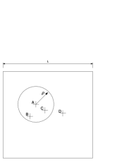
(a) Unit disk graph

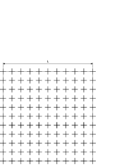
(b) Lattice

(c) Unit disk range $R$ for a lattice

Figure 1: Network Models

Precisely, the sensor networks considered will be:

• Random unit disk graphs with nodes uniformly distributed (Fig. 1(a))

• Unit disk graphs with nodes organized on a lattice (Fig. 1(b)).

An important assumption is that the wireless broadcast advantage is used: each transmission is overheard by several nodes. As a result the graph is in reality a (unit disk) hypergraph.

1.1 Related Work

In general, specifying the network coding protocol is reduced to specifying the transmission rates for each node [10]. Once the optimal rates are computed, the performance can be asymptotically achieved with distributed random linear coding, for instance [11, 4]. This article is in the spirit of [13], which starts with exhibiting an energy-efficient algorithm for simple networks. The central element for computing the performance is the estimation of the min-cut of the network and we are inspired by the existing techniques and results surrouding the expected value of the min-cut on some classes of networks: for instance, [7] explored the capacity of networks where a source is two hops from the destination, through a network of relay nodes; [8] studied some classes of random geometric graphs. Recently, [9] gave bounds of the min-cut of dual radio networks.

1.2 Network Coding

In the network coding literature, several results are for multicast, and, in this section, they are quoted as such. They apply to the topic of this article, broadcast, since broadcast is a special case of multicast.

A central result for network coding in wireless networks gives the maximum multicast rate for a source. The capacity is given by the min-cut from the source to each individual destination of the network, viewed as a hypergraph [3, 6].A precise description includes:
$\bullet$ Nodes: $\mathcal{V}=\{v_{i},i=1,\ldots{}N\}$, set of nodes of the hypergraph
$\bullet$ Hyperarc: $h_{v}=(v,H_{v})$, where $H_{v}\subset V$ is the subset of nodes that are reached by one transmission of node $v$(neighbors).
$\bullet$ Rate: Each node $v$ emits on the hyperarc $(v,H_{v})$ with rate $C_{v}$.

Let us consider the source $s$, and one of the multicast destinations $t\in\mathcal{V}$. The definition of an $s$-$t$ cut is: a partition of the set of nodes $V$ in two sets $S$, $T$ such as $s\in S$ and $t\in T$. Let $Q(s,t)$ be the set of such $s$-$t$ cuts: $(S,T)\in Q(s,t)$.

We denote $\Delta{}S$, the set of nodes of $S$ that are neighbors of at least one node of $T$; the capacity of the cut $C(S)$ is defined as the maximum rate between the nodes in $S$ and the nodes in $T$:

$$\Delta{}S\triangleq\{v\in S:H_{v}\cap T\neq\emptyset\}\leavevmode\nobreak\ \leavevmode\nobreak\ \leavevmode\nobreak\ \mathrm{and}\leavevmode\nobreak\ \leavevmode\nobreak\ \leavevmode\nobreak\ C(S)\triangleq\sum_{v\in\Delta{}S}C_{v}$$ (1)

The min-cut between $s$ and $t$ is the cut of $Q(s,t)$ with the minimum capacity. Let us denote $C_{\mathrm{min}}(s,t)$ as its capacity. From [3, 6], the maximum multicast capacity is given by the minimum of capacity of the min-cut of every destination, $C_{\mathrm{min}}(s)$, with:

$$C_{\mathrm{min}}(s,t)\triangleq\min_{(S,T)\in Q(s,t)}C(S)\leavevmode\nobreak\ \leavevmode\nobreak\ \leavevmode\nobreak\ \mathrm{and}\leavevmode\nobreak\ \leavevmode\nobreak\ \leavevmode\nobreak\ C_{\mathrm{min}}(s)\triangleq\min_{t\in\mathcal{V}\setminus\{s\}}C_{\mathrm{min}}(s,t)$$ (2)

2 Main Results

2.1 Overview

As described in the introduction, our approach is to choose an intuitive transmission rate for each node: essentially, the same rate for most nodes, as described in section 2.3. Then, we determine the maximum broadcast rate that can be achieved to transmit from the source to every node in the network as the min-cut of the hypergraph, for both random and lattice graphs in section 2.4. And finally, from the expression of the cost in section 2.5, we deduce asymptotic optimality (section 2.6).

2.2 Further Definitions

Consider a network inside a square area $G$ of edge length $L$, such as the one on Fig. 1(a).

• The radio range of the network is $\rho$.

• For a lattice, we denote $R$ the set of neighbors of the origin node $(0,0)$, as represented on Fig. 1(c): $R\triangleq\{(x,y)\in\mathbb{Z}^{2}:x^{2}+y^{2}\leq\rho^{2}\}$

• Let $M$ be the “expected” number of neighbors of one node. For a lattice, it is $M=|R|-1$. For a random disk unit graph with $N$ nodes, $M$ is related to the density $\mu=\frac{N}{L^{2}}$ and range as follows: $M=\pi\rho^{2}\mu=\pi\rho^{2}\frac{N}{L^{2}}$.

We define the border area as the area of fixed width $W>\rho$ near the edge of that square, and border nodes as the nodes in that area. Hence, the area $L\times L$ of $G$ is partitioned into:

• $\Delta{}G$, the border, with area $A_{\Delta{}G}=4W(L-W)$

• $G_{i}$, the “interior” $G_{i}\triangleq G\setminus\Delta{}G$, with area $A_{G_{i}}=(L-2W)^{2}$

2.3 Rate Selection with IREN/IRON

The principle IREN/IRON sets the following transmission rates:

• IREN (Increased Rate for Exceptional Nodes): the rate of transmission is set to $M$, for the source node and all the border nodes (the “exceptional” nodes).

• IRON (Identical Rate for Other Nodes): every other node transmits with rate $1$.

2.4 Performance: Min-Cut (Achievable Broadcast Rate)

The essence of our main result is the following property proved in section 3.1, Th. 3.4:

Property 1

With the rate selection IREN/IRON, the min-cut of a lattice graph is equal to $C_{\mathrm{min}}=M$ (with $M=|R|-1$).

For random unit disk graphs, by mapping the points to an imaginary lattice graph (embedded lattice) as an intermediary step, we are able to find bounds of the capacity of random unit disk graphs. This turns out to be much in the spirit of [9]. This is used to deduce an asymptotic result for unit disk graphs, proven in section 3.2, Th. 3.11:

Property 2

Assume a fixed range. For a sequence of random unit disk graphs $(\mathcal{V}_{i})$, with sources $s_{i}$, with size $L\rightarrow\infty$ and with a density $M\rightarrow\infty$ such as $M={}L^{\theta}{}$, for any fixed $\theta>0$, we have the following convergence in probability: $\frac{C_{\min}(s)}{M}\,{\buildrel p\over{\rightarrow}}\,1$.

2.5 Performance: Transmission Cost per Broadcast

Recall that the metric for cost is the number of (packet) transmissions per a (packet) broadcast from the source to the entire network. Let us denote $E_{\mathrm{cost}}$ as this “transmissions per broadcast.”

This cost of broadcasting with IREN/IRON rate selection can be equivalently computed from the rates as the ratio of the number of transmissions per unit time to the number of packets broadcast into the network per unit time. Then $E_{\mathrm{cost}}$ is deduced from the min-cut $C_{\mathrm{min}}$, the areas $A_{\Delta{}G},A_{G_{i}}$, the associated node rates and the node density $\mu$. For fixed $W$, $M,L\rightarrow\infty$: $E_{\mathrm{cost}}=\frac{1}{C_{\mathrm{min}}}\mu L^{2}\left(1+O(\frac{1}{L})+\frac{4MW}{L}(1+O(\frac{1}{L}))\right)$.

For random unit disk graphs, $E_{\mathrm{cost}}$ is an expected value, and $\mu=\frac{N}{L^{2}}$. For a lattice, $\mu=1$.

2.6 Near Optimal Performance for Large Networks

Sections 2.4 and 2.5 gave the performance and cost with the
IREN/IRON principle. The optimal cost is not easily computed, and in this section an indirect route is chosen, by using a bound.

Assume that every node has at most $M_{\mathrm{max}}$ neighbors: one single transmission can provide information to $M_{\mathrm{max}}$ nodes at most. Hence, in order to broadcast one packet to all $N$ nodes, at least $E_{\mathrm{bound}}=\frac{N}{M_{\mathrm{max}}}$ transmissions are necessary.

W.r.t. this bound, let the relative cost be: $E_{\mathrm{rel-cost}}=\frac{E_{\mathrm{cost}}}{E_{\mathrm{bound}}}\geq 1$.

We will prove that $E_{\mathrm{rel-cost}}\rightarrow 1$ for the following networks:

2.6.1 Lattice Graphs

For lattices, $W$ and the neighborhood $R$ are kept fixed (hence also $M=|R|-1$) and only the size $L$ of the network increases to infinity. The number of nodes is $N=L^{2}$. The maximum number of neighbors $M_{\mathrm{max}}$ is exactly $M_{\mathrm{max}}=M$.

From section 2.5 and from Property 1, we have:
$E_{\mathrm{rel-cost}}=E_{\mathrm{cost}}\frac{M_{\mathrm{max}}}{N}=\left(1+O(\frac{1}{L})+\frac{4MW}{L}(1+O(\frac{1}{L}))\right)=1+O(\frac{1}{L})$.

2.6.2 Random Unit Disk Graphs

For random unit disk graphs, first notice that an increase of the density $M$ does not improve the relative cost $E_{\mathrm{rel-cost}}$. Now consider a sequence of random graphs, as in Property 2, with fixed $\rho$, fixed $W$, and size $L\rightarrow\infty$ and with a density $M\rightarrow\infty$ such as $M={}L^{\theta}{}$, for some arbitrary fixed $\theta>0$, with the additional constraint that $\theta<1$. We have:

$E_{\mathrm{rel-cost}}=E_{\mathrm{cost}}\frac{M_{\mathrm{max}}}{N}=\frac{M}{C_{\mathrm{min}}}\frac{M_{\mathrm{max}}}{M}\frac{\mu L^{2}}{N}\left(1+O(\frac{1}{L})+\frac{4MW}{L}(1+O(\frac{1}{L}))\right)$.

Each of part of the product converges toward $1$, either surely, or in probability: using Property 2, we have the convergence of $\frac{C_{\mathrm{min}}}{M}\,{\buildrel p\over{\rightarrow}}\,1$, when $L\rightarrow\infty$ and similarly with Th. 3.11 we have $\frac{M_{\mathrm{max}}}{M}\,{\buildrel p\over{\rightarrow}}\,1$. By definition $N=\mu L^{2}$. Finally, $M={}L^{\theta}{}$ for $\theta<1$ implies that $\frac{4MW}{L}\rightarrow 0$.

As a result we have: $E_{\mathrm{rel-cost}}\,{\buildrel p\over{\rightarrow}}\,1$ in probability, when $L\rightarrow\infty$

2.6.3 Random Unit Disk Graphs without Network Coding

In order to compare the results that are obtained when network coding is not used, one can reuse the argument of [13]. Consider the broadcasting of one packet. Consider one node of the network that has repeated the packets. It must have received the transmission from another connected neighbor. In a unit disk graph, these two connected neighbors share a neighborhood area at least equal to $(\frac{2\pi}{3}-\frac{\sqrt{3}}{2})\rho^{2}$, and every node lying within that area will receive duplicate of the packets. Considering this inefficiency, for dense unit disk graphs one can deduce the following bound: $E_{\mathrm{rel-cost}}^{\mathrm{(no-coding)}}\geq\frac{6\pi}{2\pi+3\sqrt{3}}$ . Notice that $\frac{6\pi}{2\pi+3\sqrt{3}}\approx 1.6420\ldots>1$.

2.6.4 Near Optimality

The asymptotic optimality is a consequence of the convergence of the cost bound $E_{\mathrm{rel-cost}}$ toward $1$. This indirect proof is in fact a stronger statement than optimality of the rate selection in terms of energy-efficiency: it exhibits the fact that asymptotically (nearly) all the transmissions will be innovative for the receivers. Note that it is not the case in general for a given instance of a hypergraph. It evidences the following remarkable fact for the large homogeneous networks considered: network coding may be achieving not only optimal efficiency, but also, asymptotically, perfect efficiency — achieving the information-theoretic bound for each transmission.

Notice that traditional broadcast methods without network coding (such as the ones based on connected dominating sets) cannot achieve this efficiency, since their lower bound is $1.642$.

3 Proofs of the Min-Cut

3.1 Proof for Lattice Graphs

3.1.1 Preliminaries

Let $\Gamma$ be full, integer lattice in $n$-dimensional space; it is the set $\mathbb{Z}^{n}$, where the lattice points are $n$-tuples of integers.

For lattice graphs, only points on the full lattice are relevant; therefore in this section, the notations $\mathcal{L},\mathcal{L}_{i},\Delta{}\mathcal{L}$ will be used, for the parts of the full lattice $\Gamma$ that are in $G,G_{i},\Delta G$ respectively.

The proof is based on the use of the Minkowski addition, and a specific property of discrete geometry (3) below. The Minkowski addition is a classical way to express the neighborhood of one area (for instance, see [14] and the figure 3(a), and figure 4 of that reference).

Given two sets $A$ and $B$ of ${\mathbb{R}}^{n}$, the Minkowski sum of the two sets $A\oplus B$ is defined as the set of all vector sums generated by all pairs of points in $A$ and $B$, respectively: $A\oplus B\triangleq\{a+b:a\in A,b\in B\}$

Then the set of neighbors $\mathcal{N}(t)$ of one node $t$, with $t$ itself, is:
$\mathcal{N}(t)\cup\{t\}=\{t\}\oplus R$
This extends to the neighborhood of a set of points. For Minkowski sums on the lattice $\Gamma$, there exist variants of the Brunn-Minkowski inequality, including the following one [15]:

Property 3

For two subsets $A,B$ of the integer lattice $\mathbb{Z}^{n}$,

$$|A\oplus B|\geq|A|+|B|-1$$ (3)

where $|X|$ represents the number of elements of a subset $X$ of $\mathbb{Z}^{n}$

3.1.2 Bound on the capacity of one cut $C(S)$

Consider a lattice $\mathcal{L}$ and a source $s$. Let $C(S)$ be the capacity of an $s$-$t$ cut $S,T\in Q(s,t)$.

Lemma 3.1.

$C(S)\geq|\Delta{}S|$ (with $\Delta{}S$ defined in (1))

Proof 3.2.

$C_{v}\geq 1$ with IREN/IRON and with (1), $C(S)=\sum_{v\in\Delta{}S}C_{v}$

Theorem 3.3.

The capacity of one cut $C(S)$ is such that: $C(S)\geq M$

Proof: There are three possible cases, either the set $T$ has no common nodes with the border $\Delta{}\mathcal{L}$, or $T$ includes all nodes of $\Delta{}\mathcal{L}$, or finally $T$ includes only part of nodes in the border area.

First case, $T\cap\Delta{}\mathcal{L}=\emptyset$:

We know that $T\oplus R\subset\mathcal{L}$, hence we can effectively write the neighbors of nodes in $T$ as a Minkowski addition (without getting points in $\Gamma$ but out of $\mathcal{L}$): $\Delta T\triangleq(T\oplus R)\setminus T$

It follows that: $|\Delta{}T|\geq|T\oplus R|-|T|$

Now the inequality (3) can be used: $|T\oplus R|\geq|T|+|R|-1$

Hence we get: $|\Delta T|\geq|T|+|R|-1-|T|$, and therefore:

$$|\Delta T|\geq|R|-1$$ (4)

Recall that $S$ and $T$ form a partition of $\mathcal{L}$ ; and since $\Delta T$ is a subset of $\mathcal{L}$, by definition without any point of of $T$, we have $\Delta T\subset S$. Hence actually $\Delta T\subset\Delta S$ (with the definition of $\Delta S$ in (1)). We can combine this fact with lemma 3.1 and (4), to get:

$|C(S)|\geq|R|-1$ and the Th. 3.3 is proved for the first case.

The second case is similar, but considering the source, while the third case uses the fact that a path can be found in the border between any two border nodes [17]. $\Box$

3.1.3 Value of the Min-cut $C_{\mathrm{min}}(s)$

The results of the previous section immediately result in a property on the capacity of every $s$-$t$ min-cut:

Theorem 3.4.

For any $t\in\mathcal{L}$ different from the source $s$:

$C_{\mathrm{min}}(s,t)=M$ ; and as a result: $C_{\mathrm{min}}(s)=M$

Proof 3.5.

From Th. 3.3, we have the capacity of every $s-t$ cut $S/T$ verifies: $C(S)\geq M$. Hence $C_{\mathrm{min}}(s,t)\geq M$

Conversely let us consider a specific cut, $S_{s}=\{s\}$ and $T_{s}=\mathcal{L}\setminus\{s\}$. Obviously $s$ has at least one neighbor hence $\Delta{}S=\{s\}$. The capacity of the cut is $C(S_{s})=\sum_{v\in\Delta{}S}C_{v}=C_{s}=M$ and thus $C_{\mathrm{min}}(s,t)\leq M$, and the theorem follows. $\Box$

3.2 Proof of the Value of Min-Cut for Unit Disk Graphs

In this section, we will prove a probabilistic result on the min-cut, in the case of random unit disk graphs, using an virtual “embedded” lattice. The unit graph will be denoted $\mathcal{V}$, whereas for the embedded lattice the notation of section 3 is used: $\mathcal{L}$ (along with $\Delta{}\mathcal{L}$ and $\mathcal{L}_{i}$).

3.2.1 Embedded Lattice

Given the square area $L\times L$, we start with fitting a rescaled lattice inside it, with a scaling factor $r$. Precisely, it is the intersection of square $G$ and the set $\{(rx,ry):(x,y)\in\mathbb{Z}^{2}\}$.

We will map the points of $G$ to the closest point of the rescaled lattice $\mathcal{L}$: let us denote $\lambda(x)$, the application that transforms a point $u$ of the Euclidian space ${\mathbb{R}}^{2}$ to its closest point of $\mathcal{L}$. Formally, for $u=(x,y)\in\mathbb{Z}^{2}$, $\lambda(x)\triangleq(r\lfloor\frac{x}{r}+\frac{1}{2}\rfloor,r\lfloor\frac{y}{r}+\frac{1}{2}\rfloor)$

For $u\in\mathcal{L}$, $\lambda^{-1}(u)$ is the set of nodes of $\mathcal{V}$ that are mapped to $u$. The area of ${\mathbb{R}}^{2}$ that is mapped to a same point of the lattice, is a square $r\times r$ around that point.

Let $u$ be a point of the lattice $\mathcal{L}$, and let denote the $m(u)$ the number of points of $\mathcal{V}$ that are mapped to $u$ with $g$ (they are in the square around $u$ ; and $m(u)\triangleq|\lambda^{-1}(u)|$). $m(u)$ is a random variable.

Let us denote: $m_{\mathrm{min}}\triangleq\min_{u\in\mathcal{L}}m(u)\mathrm{\leavevmode\nobreak\ and\leavevmode\nobreak\ }m_{\mathrm{max}}\triangleq\max_{u\in\mathcal{L}}m(u)$

3.2.2 Neighborhood of the Embedded Lattice

We start by defining the neighborhood $R$ for the embedded lattice. We choose $R(r)$ to be the points of the lattice inside a disk of radius $\rho-2r$.

Lemma 3.6.

Let us consider two nodes of $u$, $v$ of $\mathcal{V}$ that are mapped on the lattice $\mathcal{L}$ to $u_{\mathcal{L}}$ and $v_{\mathcal{L}}$ respectively:
$\bullet$ if $u_{\mathcal{L}}$ and $v_{\mathcal{L}}$ are neighbors on the lattice, them $u$ and $v$ are neighbors on the graph $\mathcal{V}$

This results from triangle inequalities on the distances.

3.2.3 Relationship between the Capacities of the Cuts of the Embedded Lattice and the Random Disk Unit Graph

Let us consider one source $s\in\mathcal{V}$, one destination $t\in\mathcal{V}$ and the capacity of any $S/T$ cut. Every node of $S$ and $T$ is then mapped to the nearest point of the embedded lattice. For the source, we denote: $s_{\mathcal{L}}=\lambda(s)$.

An induced cut of the embedded lattice is constructed as follows:

• The border area width $W_{\mathcal{L}}$ is selected so as to be the greatest integer multiple of $r$ which is smaller than $W$ ; and $r<W-\rho$

• For any point of the lattice $v_{\mathcal{L}}\in\mathcal{L}$, the rate $C^{(\mathcal{L})}_{v_{\mathcal{L}}}$ is set according to IREN/IRON on the lattice: $C^{(\mathcal{L})}_{v_{\mathcal{L}}}=|R(r)|-1$ when $v_{\mathcal{L}}$ is within the border area of width $W_{\mathcal{L}}$, and $C^{(\mathcal{L})}_{v_{\mathcal{L}}}=1$ otherwise.

• $S_{\mathcal{L}}$ is the set including the point $s_{\mathcal{L}}$, and the points of the lattice $\mathcal{L}$ such as only nodes of $S$ are mapped to them:
  $S_{\mathcal{L}}\triangleq\{s_{\mathcal{L}}\}\cup\{u_{\mathcal{L}}:\lambda^{-1}(u_{\mathcal{L}})\subset S\}$

• $T_{\mathcal{L}}$ is the set of the rest of points of $\mathcal{L}$.

Note that $t\in T_{\mathcal{L}}$ ; that all the points of the lattice, to which both points from $S$ and $T$ are mapped, those points are in $T_{\mathcal{L}}$ ; and that the points to which no points are mapped are in $S_{\mathcal{L}}$: $S_{\mathcal{L}}/T_{\mathcal{L}}$ is indeed a partition and a $s_{\mathcal{L}}-t_{\mathcal{L}}$ cut.

Lemma 3.7.

The capacity $C(S)$ of the cut $S/T$ and the capacity of the induced cut $C^{(\mathcal{L})}(S_{\mathcal{L}})$ verify: $C(S)\geq m_{\mathrm{min}}C^{(\mathcal{L})}(S_{\mathcal{L}})$

This comes from the fact that neighborhood on the lattice implies neighborhood in $\mathcal{V}$ (lemma 3.6), and then an inclusion is proved between the $\Delta{}S_{\mathcal{L}}$ of the capacity of cut of the lattice from (2) and the $\Delta{}S$ of the cut $S/T$ [17].

Theorem 3.8.

The min-cut $C_{\mathrm{min}}(s)$ of the graph $\mathcal{V}$, verifies:

$C_{\mathrm{min}}(s)\geq m_{\mathrm{min}}(|R(r)|-1)$

Proof 3.9.

From lemma 3.7, any cut $C(S)$ is lower bounded by $m_{\mathrm{min}}C^{(\mathcal{L})}(S_{\mathcal{L}})$. Since $C^{(\mathcal{L})}(S_{\mathcal{L}})$ is the capacity of a cut of a lattice with IREN/IRON, Th. 3.4 also indicates that: $C^{(\mathcal{L})}(S_{\mathcal{L}})\geq C^{(\mathcal{L})}_{\mathrm{min}}(s_{\mathcal{L}})=|R(r)|-1$. Hence the lower bound $m_{\mathrm{min}}(|R(r)|-1)$ for any $C(S)$, and therefore for the min-cut $C_{\mathrm{min}}(s)$.

3.2.4 Nodes of $\mathcal{V}$ Mapped to One Lattice Point

In Th. 3.8, $m_{\mathrm{min}}$ plays a central part. Let us start with $m(u_{\mathcal{L}})$: it is actually a random variable that is the sum of $N$ Bernoulli trials. With a Chernoff tail bound [16], we get, for $\delta\in]0,1[$:
$Pr[m(u_{\mathcal{L}})\leq(1-\delta)E[m(u_{\mathcal{L}})]]\leq\exp(-\frac{E[m(u_{\mathcal{L}})]\delta^{2}}{2})$

A bound on $m_{\mathrm{min}}$ is deduced from the fact that it is the minimum of $m(u)$ and from the fact that for two events $A$ and $B$,
$Pr[A$ or $B]\leq Pr[A]+Pr[B]$:

Theorem 3.10.

$Pr[m_{\mathrm{min}}\leq(1-\delta)\mu r^{2}]\leq\exp\left((\log\frac{L^{2}}{r^{2}})(1-\frac{\mu r^{2}\delta^{2}}{2\log\frac{L^{2}}{r^{2}}})\right)$

3.2.5 Asymptotic Values of the Min-Cut of Unit-Disk Graphs

Theorem 3.11.

For a sequence of random unit disk graphs and associated sources $(\mathcal{V}_{i},s_{i}\in\mathcal{V}_{i})$, with fixed radio range $\rho$, fixed border area width $W$, with a size $L_{i}\rightarrow\infty$, and a density $M=L^{\theta}$ with fixed $\theta>0$, we have the following limit of the min-cut $C_{\mathrm{min}}(s_{i})$:
$\frac{C_{\mathrm{min}}(s_{i})}{M}\,{\buildrel p\over{\rightarrow}}\,1\mathrm{\leavevmode\nobreak\ in\leavevmode\nobreak\ probability.\leavevmode\nobreak\ Additionally:\leavevmode\nobreak\ }\frac{M_{\mathrm{max}}}{M}\,{\buildrel p\over{\rightarrow}}\,1$

Proof 3.12.

Notice that $Pr[m_{\mathrm{min}}>\mu r^{2}]=0$, because otherwise we would have a minimum of some values $m(u_{\mathcal{L}})$ greater than their average. Starting from Th. 3.10, several variables appear: $L$, $\mu$, $\delta$, and $r$. Assume that $\rho$ is fixed and that $\mu=KL^{\theta}$ for some fixed $\theta>0$ and $K>0$. Then we propose the following settings: $\delta=L^{-\frac{\theta}{8}}$ ; $r=L^{-\frac{\theta}{8}}$

As a result, from Th. 3.10 we have: $\frac{m_{\mathrm{min}}}{\mu r^{2}}\,{\buildrel p\over{\rightarrow}}\,1$. Now Th. 3.8 gives:
$C_{\mathrm{min}}(s)\geq m_{\mathrm{min}}(|R(r)|-1)$. Hence: $\frac{C_{\mathrm{min}}(s)}{M}\geq\frac{m_{\mathrm{min}}}{\mu r^{2}}\frac{\mu}{M}r^{2}(|R(r)|-1)$
From the fact that $|R(r)|=\pi(\frac{\rho}{r})^{2}+O(\frac{1}{r})$ [17], and that $M=\pi\rho^{2}\mu$, we get the lower bound $1$ for the limit of $\frac{C_{\mathrm{min}}}{M}$. The upper bound comes indirectly from the fact that $\frac{M_{\mathrm{max}}}{M}\,{\buildrel p\over{\rightarrow}}\,1$ [17]. $\Box$

4 Conclusion

We have presented a simple rate selection for network coding for large sensor networks. We computed the broadcast performance from the min-cut with networks modeled as hypergraphs. The central result is that selecting nearly the same rate for all nodes achieves asymptotic optimality for the homogeneous networks that are presented, when the size of the networks becomes larger. This can be translated into this remarkable property: nearly every transmission becomes innovative for the receivers. As a result, it was shown that network coding would asymptotically outperform any method that does not use network coding. We believe that the results presented here are a first step for a simple but efficient rate selection in wireless sensor networks in the plane. Future research work will determine how to adapt the rate selection for smaller and less homogeneous networks.

1

References

- [1] R. Ahlswede, N. Cai, S.-Y. R. Li and R. W. Yeung, “Network Information Flow”, IEEE Trans. on Information Theory, vol. 46, no.4, pp. 1204-1216, Jul. 2000
- [2]
- [3] A. Dana, R. Gowaikar, R. Palanki, B. Hassibi, and M. Effros, “Capacity of Wireless Erasure Networks”, IEEE Trans. on Information Theory, vol. 52, no.3, pp. 789-804, Mar. 2006
- [4] D. S. Lun, M. Médard, R. Koetter, and M. Effros, “On coding for reliable communication over packet networks”, Technical Report #2741, MIT LIDS, Jan. 2007
- [5] Y. Wu, P. A. Chou, and S.-Y. Kung, “Minimum-energy multicast in mobile ad hoc networks using network coding”, IEEE Trans. Commun., vol. 53, no. 11, pp. 1906-1918, Nov. 2005
- [6] D. S. Lun, N. Ratnakar, M. Médard, R. Koetter, D. R. Karger, T. Ho, E. Ahmed, and F. Zhao, “Minimum-Cost Multicast over Coded Packet Networks”, IEEE/ACM Trans. Netw., vol. 52, no. 6, pp 2608-2623, Jun. 2006
- [7] A. Ramamoorthy, J. Shi, and R. D. Wesel, “On the Capacity of Network Coding for Random Networks”, IEEE Trans. on Information Theory, Vol. 51 No. 8, pp. 2878-2885, Aug. 2005
- [8] S. A. Aly, V. Kapoor, J. Meng, and A. Klappenecker, “Bounds on the Network Coding Capacity for Wireless Random Networks”, Third Workshop on Network Coding, Theory, and Applications (Netcoding07), Jan. 2007
- [9] R. A. Costa and J. Barros. “Dual Radio Networks: Capacity and Connectivity”, Spatial Stochastic Models in Wireless Networks (SpaSWiN 2007), Apr. 2007
- [10] D. S. Lun, M. Médard, R. Koetter, and M. Effros, “Further Results on Coding for Reliable Communication over Packet Networks” International Symposium on Information Theory (ISIT 2005), Sept. 2005
- [11] T. Ho, R. Koetter, M. Médard, D. Karger and M. Effros, “The Benefits of Coding over Routing in a Randomized Setting”, International Symposium on Information Theory (ISIT 2003), Jun. 2003
- [12] B. Clark, C. Colbourn, and D. Johnson, “Unit disk graphs”, Discrete Mathematics, Vol. 86, Issues 1-3, Dec. 1990
- [13] C. Fragouli, J. Widmer, and J.-Y. L. Boudec, “A Network Coding Approach to Energy Efficient Broadcasting”, Proceedings of INFOCOM 2006, Apr. 2006
- [14] I.K. Lee, M.S. Kim, G. Elber, “Polynomial/Rational Approximation of Minkowski Sum Boundary Curves”, Graphical Models and Image Processing, Vol. 69, No. 2, pp 136-165, Mar. 1998
- [15] R. J. Gardner, P. Gronchi, “A Brunn-Minkowski inequality for the integer lattice”, Trans. Amer. Math. Soc., 353 (2001), 3995-4042
- [16] P. Barbe, M. Ledoux, Probabilité Editions Espaces 34, Belin, 1998.
-
[17]
C. Adjih, S. Y. Cho, P. Jacquet,