Visualization of Cosmological Particle-Based Datasets

Abstract

We describe our visualization process for a particle-based simulation of the formation of the first stars and their impact on cosmic history. The dataset consists of several hundred time-steps of point simulation data, with each time-step containing approximately two million point particles. For each time-step, we interpolate the point data onto a regular grid using a method taken from the radiance estimate of photon mapping [21]. We import the resulting regular grid representation into ParaView [24], with which we extract isosurfaces across multiple variables. Our images provide insights into the evolution of the early universe, tracing the cosmic transition from an initially homogeneous state to one of increasing complexity. Specifically, our visualizations capture the build-up of regions of ionized gas around the first stars, their evolution, and their complex interactions with the surrounding matter. These observations will guide the upcoming James Webb Space Telescope, the key astronomy mission of the next decade.

I.3.6Computing MethodologiesComputer GraphicsMethodology and Techniques; J.2Computer ApplicationsPhysical Sciences and EngineeringAstronomy

Introduction

One of the most important open questions in modern cosmology is to understand how the first stars in the universe, formed a few 100 million years (100 Myr) after the Big Bang, ended the so-called “cosmic dark ages” [4]. The first stars transformed the early universe from its simple, homogeneous initial state to one of increasing complexity, thus setting the stage for the entire subsequent history of structure and galaxy formation. This crucial transformation is concerned with two interrelated processes: the re-ionization of the universe, and the enrichment with heavy chemical elements. The universe before the formation of the first stars consisted of neutral, almost pure hydrogen and helium gas. Prior to the first stars, there were no sources of ultraviolet (UV) photons yet, which are required to ionize hydrogen, and the cosmic gas was completely neutral at this early time. Observations, however, have shown that the universe was again highly ionized, at least beginning one billion years after the Big Bang. How this so-called re-ionization happened is a primary focus of current cosmological debate. The universe underwent a second formative transformation at the end of the dark ages, when the pristine cosmic gas, containing only the hydrogen and helium produced in the Big Bang, was enriched with heavy chemical elements that were synthesized in the first stars, and subsequently dispersed in extremely energetic supernova explosions. The first stars, therefore, began the long nucleosynthetic process that resulted in all the heavy elements that we find in our Solar System today.

Both of these cosmic transformations were highly complex, involving the three-dimensional evolution of dark matter and gas, coupled together by gravity. Furthermore, studying the impact of the first stars on their surroundings requires a radiation-hydrodynamics calculation, which is at the frontier of what is currently feasible. Progress can therefore only be made with sophisticated, large-scale numerical simulations. Specifically, we use a Lagrangian, particle-based technique to evolve the cosmic gas, the so-called smoothed particle hydrodynamics (SPH) algorithm. Gravitational forces, acting on both gas and dark matter, are solved with a hierarchical tree method. Our code has been parallelized with the Message-Passing Interface (MPI) library, and performs well on large Beowulf-type systems.

From this simulation, we want to produce images of smooth isosurfaces that represent the various gas structures present. The particle data from the simulation has unknown structure, which hinders direct extraction of isosurfaces. Instead, we use an interpolation similar to the three-dimensional radiance estimation technique from photon-mapping [21] to interpolate the particle data to the vertices of a regular grid. In our process, the user may define the grid resolution and sampling range, which allows data to be represented at various levels of detail. With data on a regular grid, we can use any of a variety of open-source software tools to extract and view the isosurfaces. For the images presented here we use ParaView [24], which provides a feature-rich set of tools to create and enhance our images, including isosurface extraction and smoothing.

A key aspect of current research on the first stars is related to the build-up and growth of bubbles of either ionized gas or hot, heavy element-enriched gas. Our visualizations are crucial to elucidate the evolution of the bubbles, their complex interaction with the surrounding medium, and the time-dependent topology of multiple bubble growth and overlap. Other visualization techniques do not produce images that clearly demonstrate these phenomena. Our numerical simulations, coupled with the effective visualization techniques that we describe here, will allow us to make predictions for the James Webb Space Telescope (JWST), planned for launch in $\sim 2013$. The JWST, the key astronomy mission in the next decade, is extremely sensitive at near-infrared (NIR) wavelengths, where most of the light from the first stars, emitted at the source in the UV, but subsequently redshifted by the cosmic expansion into the NIR, is expected to reside.

The remainder of the paper is organized as follows: in Section 1 we present the cosmological motivation for our visualization; in Section 2 we describe our visualization process, and in Section 3 we discuss the insights made possible by our visualizations. We present related work in Section 4 and future work in Section 5.

Figure 1: Regions Ionized by the First Three Stars — This figure shows the ionized gas within the first three ionized regions. A region containing an active star is on the left, while in the two regions on the right the central stars have turned off and the electron fraction is dropping as the gas recombines. Three isosurfaces of the electron fraction are shown: 0.34 (cyan), 0.10 (orange) and 0.01 (blue). The structures in the two right-most bubbles demonstrate that ionized gas cools and recombines non-uniformly, again becoming neutral. It was often previously assumed that the gas recombined in a homogeneous fashion, with the electron fraction roughly equal throughout the ionized regions.

1 Cosmological Background

1.1 Simulations

To study how the formation of the first stars affects the early universe, we carry out detailed three-dimensional simulations of a large volume of the cosmos during the epoch of the formation of the first generation of stars. These simulations allow us to follow the evolution of the primordial gas as it collapses under the influence of gravity to form stars, and as the radiation from these stars, in turn, alters the chemistry and thermal state of the gas[22].

1.1.1 Smoothed Particle Hydrodynamics

We carry out our simulations using the smoothed-particle hydrodynamics (SPH) code GADGET, in which the gas is modeled as discrete particles, each of which carries information about the dynamical, thermal, and chemical properties of the gas at a given point [38, 37]. The mass contained in a given particle, however, is smoothed out over a volume that depends on the mass density and the numerical resolution. Variables at any given point in the fluid, and not only at the location of the particles, can then be estimated by kernel interpolation. Our simulation uses $\sim$ 2 million SPH particles, along with $\sim$ 2 million dark matter particles, which capture the gravitational effects that dark matter imposes. The volume of our cosmological simulation is a cubic box with side length 460 kpc $(1+z)^{-1}$ $h^{-1}$, where $z$ is the cosmological redshift, which decreases with time as the universe expands, and $h=0.7$ is the Hubble constant in units of 100 km s^-1 Mpc^-1, which describes the rate of the cosmic expansion.

We initialize our simulation at a redshift of $z=99$, when the primordial gas is nearly uniformly distributed across space and each SPH particle modeling the gas has a density, temperature, and chemical abundances as derived from Big Bang theory and cosmological observations. As the gas in our cosmological volume evolves, we track the detailed evolution of the gas as it collapses, cools, and begins to form stars at a redshift $z\sim 20$, or $\sim 200$ million years after the Big Bang.

1.1.2 Radiation From the First Stars

We model the effects of the radiation from the first generations of stars by placing point sources of radiation at the sites in our simulation where the gas collapses to high densities under the influence of gravity. The radiation from the first stars has two important effects on their surroundings, the ionization and concomitant heating of the primordial gas, and the destruction of the H₂ molecules in the gas, which are important coolants allowing the gas to collapse and form stars. The gas within a few kiloparsecs of the star is ionized and heated to temperatures above $\sim 10^{4}$ K, whereas the H₂ in the gas is destroyed within a slightly larger region around the star.

We use a ray-tracing method to find the exact structure of these two regions around the sites of star formation in our simulation. Within the so-called H II region, inside of which the gas is completely ionized, we set the electron fraction of the gas to unity and raise the temperature of the gas accordingly. Within the Lyman-Werner (LW) bubble, the region in which the molecules in the gas are destroyed, we set the fraction of H₂ to zero. Because the first stars are expected to have been very massive, with masses perhaps 100 times that of the Sun, we take it that the stars in our simulation have correspondingly short lifetimes of 3 Myr. Thus, after this brief stellar lifetime has elapsed in our simulation, we allow the gas to evolve once more without any radiative effects. In our simulation, eight stars are formed in the course of 50 Myr, and we carry out this detailed process of including the radiative effects for each of these stars.

1.2 Data Types

Each of the SPH particles that we use to model the primordial gas carries all of the relevant information that we would like to know about the dynamical, thermal, and chemical properties of the gas. In particular, each of these particles tracks the location, temperature, density, molecule (H₂) fraction, and electron fraction of a given parcel of gas. It is these properties of the primordial gas which are perhaps the most important to know in order to understand the process of the formation of the first stars and protogalaxies. Therefore, we have focused on visualizing these properties of the gas as they vary within our cosmological box, in order to extract an understanding of some of the many phenomena that arise with the feedback imposed by the first generations of stars.

Figure 2: Technique Comparison — here we compare the image quality between direct visualizations, which are often used for cosmological data sets, and our isosurface visualization. All three images show the density field in our simulation, while the middle and right images also show the electron fraction in ionized regions. The left image was generated directly from our particle data using alpha-blended sprites in Partiview [26]. The middle and right images were generated in ParaView [24]. The middle image is a direct visualization of the particle data as points. The right image was generated by resampling our particle data to a regular grid using the interpolation we describe in Section 2. We then use ParaView [24] to extract and smooth the isosurfaces. In the right image, the full extent of the gas structures are visible, and the spatial relationships among the structures are clearly defined. Note that the transparency of the isosurfaces provides additional structural information without sacrificing the clarity of the spatial relationships. Partiview image courtesy of Karla Vega, Texas Advanced Computing Center.

2 Visualization Process

The most effective visualization of our particle simulation will show the detailed structure of the gases and their spatial relationships. In particular, we would like to observe whether the ionized “bubbles” form in regions of high molecular density, and if hydrogen is suppressed in areas of active ionization. We would also benefit if the visualization revealed details of our simulation that we did not expect. Further, we seek a visualization process that is quick to implement and utilizes as much existing freely available, open-source software as possible.

In this section, we describe both our visualization techniques and the considerations that motivated the techniques. We hope that in so doing we can inform the decision-making process of other researchers faced with similar challenges. We first present other visualization techniques we considered and the reasons why we did not ultimately use them. We follow with the presentation of our chosen visualization techniques. We describe the cosmological insights made possible by our visualizations in Section 3.

2.1 Other Techniques Considered

We considered several visualization techniques other than our technique described in Section 2.2. We discuss both direct point visualization techniques and other isosurface extraction techniques.

2.1.1 Direct Point Visualization Techniques

We tested two forms of direct point visualization: visualizing the simulation particles as points using ParaView [24] and visualizing the particles with alpha-blended sprites at each particle location using Partiview [26]. Figure 2 contains example images from each technique. Because of the discrete nature of the particle simulation, these visualizations only imply the extent of the gas structures we wish to observe. The visualizations lack the clear structural detail necessary for scientific work. It is also difficult to see the spatial relationships among features, even when interacting with the visualization in three dimensions.

To define the complete extent of the gas structures in our simulation, we must select an isosurface extraction technique.

2.1.2 Isosurface Extraction Techniques

Most isosurface extraction techniques operate only on a grid, whether structured or unstructured [27]. Our particle simulation produces a point cloud with no explicit order or connectivity information, which complicates using an unstructured grid representation for isosurface extraction. Techniques exist [8] to extract isosurfaces directly from point clouds, but we are unaware of any open-source implementations. For our purposes, the potential information gain from such techniques does not overcome the implementation cost. We can achieve sufficient visualization quality from isosurface techniques that operate on a regular grid. Therefore, we will focus on resampling our data to a regular grid.

While there are many isosurface extraction techniques, we would like to use one with a well-tested, freely-available implementation. If such an implementation can meet our needs, we can eliminate potential delays and errors from implementing a technique ourselves. Ideally, the implementation would be part of a complete visualization package so we may immediately proceed with data exploration rather than implementing image rendering and user interface code.

While many visualization packages implement isosurface extraction techniques, few contain any resampling methods. The Visualization ToolKit (VTK) [23] contains only two, the most appropriate of which is an implementation of Shepard’s method [36]. However, this interpolation is a global technique, which means every point in the original data set is included in the computation for each interpolation point. This process is order $n^{2}$, where $n$ is the number of points in the original data set, and is unacceptably slow when $n$ is large. We want an interpolation that provides acceptable fidelity to the original data along with the ability to control how much of the original data is included in the computation for each interpolation point.

Figure 3: Our Local Interpolation Method — we show four toy cases to illustrate how our interpolation method works for distance $d=2$ and $n=5$, projected into two dimensions. In (A), exactly five particles are within the sampling radius $d$, and these five particles are used in the interpolation. In (B), only three particles are within the sampling radius, so only these three particles are used. In (C), there are eight particles within the sampling radius, so only the five ($n=5$) closest are used. In (D), no particles are within the sampling radius, so a set of default values are put at the interpolation point. For the results presented here, we used zeros for the scalar variables at such points.

2.2 Our Visualization Technique

Our chosen visualization technique borrows an interpolation used in computer graphics to resample our particle data to a regular grid, then uses a well-tested, freely available visualization package to extract isosurfaces and create visualization images. While a quantitative analysis of our technique is beyond the scope of this paper, we provide the rationale that motivates our parameter choices and the impact different values would have.

Our interpolation comes from the radiance estimation technique in Jensen’s photon mapping algorithm [20], a global illumination technique in computer graphics. In photon mapping, radiance samples are propagated from light sources to surfaces in a scene prior to any visibility calculations. The radiance at each sample is calculated using the luminance properties of the light source, the surface material properties, and the distance and angle between light and surface. These radiance samples are stored in a spatial acceleration structure. When rendering the scene, the indirect diffuse illumination on a surface is estimated by interpolating among the radiance samples near the visibility sample point. Jensen and Christensen [21] extend this technique to sample radiance in three dimensions, both on surfaces and in participating media. We adapt this three-dimensional interpolation technique to resample our particle data to a regular grid.

This sort of interpolation has been described as a localized inverse distance-weighted method [13] and as an $n^{th}$-nearest neighbor density estimate [21].

Our interpolation process performs the following steps: 1) determine grid resolution; 2) insert particles into grid; and 3) interpolate data to grid vertices. We input the resulting regular grid into our chosen visualization package to extract isosurfaces and create the visualization images.

2.2.1 Determining Grid Resolution

The grid resolution of the interpolation directly affects the information quality of the visualization and the efficiency of the visualization process. An overly coarse grid will not capture high-frequency details in the original data set, while an overly fine grid will consume extra memory and computing resources without expressing any new information. The ideal grid resolution is no more than half the size of the smallest expected feature [10].

If we do not know the ideal grid resolution, we calculate a reasonable grid resolution using the global point density in the original data set. First, we determine a reasonable number of grid cells per unit distance ($cpud$) with the equation [32]

$$cpud=\frac{c\,n^{\frac{1}{3}}}{\Delta_{major\_axis}}\,length_{major\_axis}$$ (1)

where $n$ is the number of particles in the original data set, $\Delta_{major\_axis}$ is the length of the longest axis of a bounding box around the original data set, and $c$ is an experimentally derived constant. For this paper, we found $c=1$ provides sufficient grid resolution to capture relevant features in our data.

To calculate the grid resolution, our process takes the bounding box around the original data set and multiplies the length of each size by $cpud$. This makes the resulting cells as cube-like as possible so that our interpolation is as uniform as possible.

For initial data exploration, we can use an artificially coarse grid resolution to create a smaller data set. Coarse grids have less data and thus isosurfaces can be extracted and visualized more quickly. Visualizing such a ’prototype’ grid can be a useful way to determine exact isovalues and view positions before visualizing for all desired details on a finer grid.

For this paper, we used a $128\times 128\times 128$ grid, which produced good visualizations in a reasonable amount of time. Higher resolutions increased the data size and processing time without a significant increase in visualization quality, while lower resolutions produced insufficiently accurate visualizations. Note that all axes contain the same number of cells because the extent of our data set is cube-shaped. If the extent of a data set is more rectangular, the grid axes may have different number of cells.

2.2.2 Particle Insertion

Once the grid resolution has been determined, our process inserts particles into grid cells according to their location in space. The insertion process is similar to inserting geometry in a grid acceleration structure in computer graphics [14]. Since our interpolation points are located at the grid vertices, our process uses the cells near a vertex to quickly eliminate particles that need not be included in the interpolation for that vertex. Our process can eliminate from consideration all particles in a cell that falls outside the local interpolation region (see Section 2.2.3 below).

2.2.3 Interpolation

After the particles have been inserted into the grid, we perform an inverse-distance weighted interpolation at each grid vertex. For each vertex, we would like to achieve a sufficiently-accurate interpolation while using a minimal number of particles. Specifically, we wish to eliminate distant particles that only marginally affect the interpolation result. Thus we can calculate a close approximation of a global interpolation with much less computation.

We control the number of particles used in the interpolation by specifying both an inclusion distance $d$ for particles around the interpolation point and a maximum number of particles $n$ that can be included in the interpolation at each point. The distance parameter $d$ must be set large enough so that we expect a sufficient number of particles to be included for the interpolation steps. Yet, a reasonable value for $d$ may include far more particles than expected in a region of high particle density. Therefore, we also set a maximum number of particles $n$ that can be included in the interpolation, so that the computation is still efficient. For such cases, we include the closest $n$ particles to the interpolation point. Because our process enforces the $n$ particle limit only in dense regions, we do not expect to compromise the quality of the interpolation. The limit only enforces the expected particle count implied by $d$.

Note that if a global interpolation is desired, $d$ can be set equal to the major axis of the bounding box of the original data set and $n$ can be set equal to the total number of particles in the original data set. Thus, every particle would be included in the interpolation at each interpolation point.

Figure 3 demonstrates the four possible ways in which $d$ and $n$ control the number of particles included at each interpolation point. For the case where no particles fall within the inclusion distance $d$ (case D in the figure), a default value for each interpolation variable is used. For this paper, we use zero.

Values of $d$ and $n$ should be selected according to the quality of the interpolation desired. Larger values for $d$ globally improve the interpolation, and larger values for $n$ improve the interpolation for dense regions of the original data set. For this paper, we set $d$ equal to the width of one grid cell ($d=3.62$) and we set $n$ equal to one percent of the total particle count ($n\approx 20K$). These values are experimentally determined, where larger values do not noticeably improve the quality of the interpolation for our purposes.

2.2.4 Isosurface Extraction and Visualization

After the interpolation is performed, we import the resulting regular grid into ParaView [24] to extract and smooth the isosurfaces. We choose ParaView because it is a well-tested, full-featured and open-source visualization package. Thus we can begin visualizing our data immediately rather than spending additional effort implementing and debugging an ad-hoc solution.

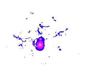
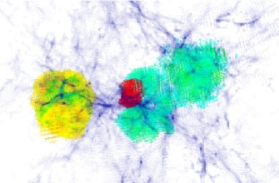
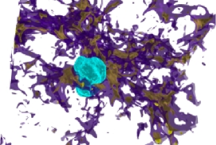
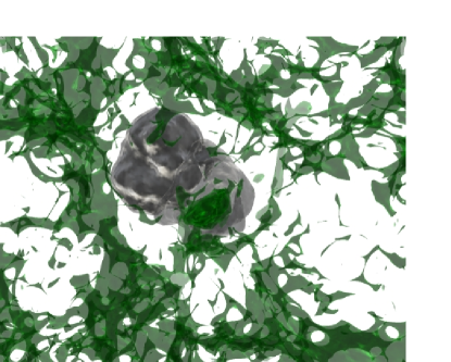
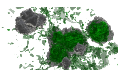
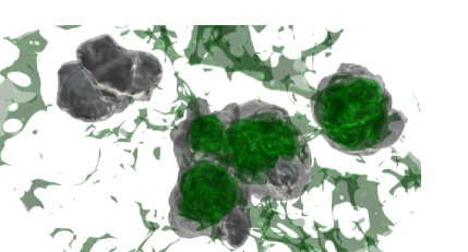
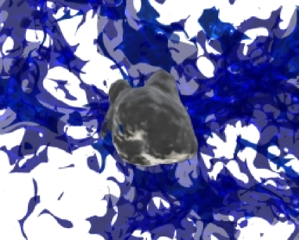
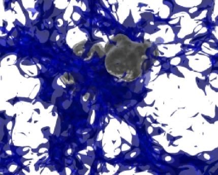
We use Marching Cubes [30] to generate our isosurfaces. To ensure all isosurfaces are visible, we create only two to three isosurfaces per visualized variable. Low-value isosurfaces are colored darker and have greater transparency (lower alpha), whereas high-value isosurfaces are colored lighter and have greater opacity (higher alpha). For two-isosurface images, we use alpha values of $0.4$ and $0.8$; for three-isosurface images, we use alpha values of $0.3$, $0.5$, and $0.8$. We select power-of-two increments for isosurface hue (e.g., 64, 128, 255), to visually distinguish isosurfaces of the same variable. In general, we use a standard color scheme to easily identify the variables in the visualization (green for hydrogen density, blue for molecular density, gray for ionized molecules; see Figures 4, 5, and 6); however, for dramatic effect in stand-alone images, we select high-contrast hues (see Figures 1 and 2).

After creating the isosurfaces, we apply a smoothing filter to remove noise and insignificant surfaces from the isosurface extraction. We use 1000 iterations of the smoothing filter for the images in this paper. In Figure 5, we demonstrate the improvement in image quality that the smoothing filter provides. It is easier to see the significant structures in the smoothed image, and the spatial relationships among the structures are more readily apparent.

ParaView also incorporates animation controls, with which we create image sequences across our data sets. By creating a time series in ParaView, we create the desired isosurfaces for one time step and generate tens to hundreds of images across the sequence. The video submitted with this paper was assembled from frames generated by ParaView.

3 Results and Discussion

The visualizations produced by our technique provide us with critical insight into the structure and spatial organization of the gases in our simulation, which furthers our cosmological understanding and the impact of our work. We describe several of these cosmological insights below. For more detail about the cosmology, we refer readers to Johnson et al. [22].

Figure 4: Hydrogen Ionization — This figure shows an active and a “ghost” ionized region, where recombination is taking place and the gas is again becoming neutral, along with the molecular hydrogen (H₂) fraction within our simulation. Ionized gas isosurfaces $5e^{-2}$ (opaque) and $5e^{-3}$(transparent) are in gray, and hydrogen density isosurfaces $3e^{-6}$, $1e^{-5}$, and $1e^{-4}$ are in green Notice that the H₂ fraction is suppressed around the active ionized region, but is instead elevated within the “ghost” ionized region.

Figure 5: Isosurface Extraction and Smoothing — These figures show several active and one “ghost” ionized region, wherein recombination is taking place and the gas is again becoming neutral, along with the molecular hydrogen (H₂) fraction within our simulation. The top image contains raw isosurfaces, and the bottom image contains isosurfaces after the application of a smoothing filter. The smoothing filter sharpens the significant structures and removes the insignificant structures, making the spatial relationships among the structures more readily apparent.

Figure 6: Formation of Ionized Regions — This figure shows the density field when the first star has formed (top) and after a second and third star have formed (bottom). Notice that in the bottom image, the first star has turned off and only the “ghost” ionized region is present (partially obscured by the molecular density isosurfaces). Ionized gas isosurfaces $5e^{-2}$ (opaque) and $5e^{-3}$(transparent) are in gray, and density isosurfaces $1.1e^{-2}$ and $5e^{-3}$ are in blue. Notice that the second and third stars have formed in the densest regions, as expected.

3.1 Cosmological Insights

The key question for cosmology is to understand the fundamental transition in the early universe from simplicity to complexity, brought about by the first stars. Specifically, how was the universe re-ionized, and how was it enriched with the first heavy elements? Understanding the build-up of ionized regions around the first stars is important for a number of reasons. Firstly, the evolution of the ionized bubbles, the speed with which they grow, and the final size reached, are diagnostic of the properties of the first stars, in particular their mass. The typical mass of the first stars is currently only predicted by theory, and it is essential to devise empirical tests. One such test is to carry out simulations of the early re-ionization process, assuming different stellar masses, and to trace and characterize the resulting pattern of ionized bubbles. The observational signature includes the three-dimensional arrangement of the bubbles, their clustering properties, and their overall volume filling fraction as a function of time. Visualizations are crucial to glean this signature from the numerical simulations. Our visualizations have shown that the bubble interior is not uniformly ionized (see Figure 1); instead there are pockets of high-density gas inside of them that remain substantially neutral. We find that higher mass stars tend to result in more homogeneous bubble interiors. In addition, higher mass stars produce larger ionized bubbles that fill a larger fraction of the available cosmic volume. Note that the structural detail found in our isosurface visualizations enables these observations, observations that are not possible with direct visualization on the particles.

Secondly, the build-up of bubbles is related to what is termed “radiative feedback”. The basic idea is that stars can only form out of cold, dense gas. Once the first stars have formed, they ionize and heat the surrounding medium, so that no other, secondary stars can form for a substantial amount of time. Put differently: wherever the ionized bubbles extend, further star formation is suppressed. Visualizing the network of radiation bubbles is therefore crucial to characterize the strength of this negative feedback. More precisely, there are two different kinds of radiation bubbles surrounding the first stars: hard UV photons that are capable of ionizing hydrogen atoms, and somewhat less energetic, soft UV photons that are capable of dissociating hydrogen molecules. The latter are very important, because they cool the primordial gas, thus enabling the formation of the first stars. The extent of the soft-UV bubbles thus delineates regions where no stars can form. We find the surprising result that soft UV photons seem much less effective in shutting off secondary star formation than was previously thought. Our visualizations clearly show the relation of the two classes of UV bubbles: The soft UV bubbles are larger than the hard UV ones, but, surprisingly, only slightly so, as can be seen in Figure 4. As this figure demonstrates, the smoothing filter and transparency used in our visualization is essential for drawing new cosmological insights.

A related question concerns the overall time evolution of early re-ionization. Traditionally, it has been argued that re-ionization is a strictly monotonous process. The fraction of the volume filled by ionized bubbles was thought to only increase with time. Our work has shown that the early stages of re-ionization occur in a much more complex fashion, where bubbles grow, disappear again, and are eventually replaced by new bubbles. The time evolution, therefore, is highly intermittent, and not at all monotonic. This effect can be seen in Figure 6, where the ionized region of the first star has been largely replaced by the ionized regions of the second and third star. Note that these observations cannot be made without seeing the spatial relationships that are made clear in our visualizations.

Our visualizations also have allowed us to understand this intermittency more fully. Specifically, we find that the bubbles do not disappear completely after the star that produced them has died; instead, a remnant of reduced, but still significant, ionization lingers on for a long time (see Figure 1), so that a given point in space can be influenced simultaneously by such a “ghost” bubble, together with a freshly formed bubble around a star that is still alive, as can be seen in Figures 4 and 6. Again, the observational signature form the early re-ionization, which depends on the precise degree of ionization, looks substantially different because of this “ghost” effect. Transparency and smoothing are necessary to observe these structural details.

An effect related to the intermittecy of the ionization at the early stages of star formation is the production of a high molecular hydrogen (H₂) fraction within the “ghost” ionized regions. This occurs because the small degree of ionization that lingers in these regions allows for free electrons to catalyze the production of H₂. The high fraction of H₂ that develops in one of these regions can be seen in Figure 4, where the highest H₂ fraction is clearly shown within the “ghost” ionized region in the middle of our simulation box. Because molecules are effective coolants of the gas, these regions may be the sites of continued star formation, a further illustration of how the UV radiation from the first stars is surprisingly ineffectual at suppressing star formation.

4 Related Work

In this section, we discuss related cosmological visualizations, isosurface extraction techniques and interpolation techniques. We motivate the choices we made when designing our technique.

4.1 Cosmological Visualizations

Researchers have often visualized cosmological phenomena, but they usually visualize their particle simulation directly. To our knowledge, there is no work that summarizes the various techniques and their applications. We discuss the work most relevant to ours below.

ParaView [24] has been used recently to compare the results of several cosmological simulations [1, 19]. These direct particle visualizations demonstrate the power and flexibility of using a well-tested, open-source visualization package. Indeed, the large community of developers that contribute to open-source, general visualization packages help ensure that recent visualization advances are included quickly. Dedicated astronomical or cosmological visualization packages often lack features or robustness. For instance, Partiview [26] lacks isosurfacing capability and our data set was too large for AstroMD [12]. AstroMD, like ParaView, is based on VTK [23], but its development has stagnated (last update in 2004) and it lacks the abilities and easy use of a more mature system.

4.2 Isosurface Extraction

Most isosurface extraction methods operate only on structured data usually a structured or unstructured grid [27]. Livnat [27] and Sutton et al. [39] provide overviews of popular isosurface extraction techniques.

Marching Cubes [30] is the most well-known isosurface extraction techniques. Marching Cubes is relatively simple to implement, but it requires a structured grid from which to create the isosurfaces. The original implementation relies on a uniform grid, but octree-based optimizations also exist [41].

Value-space decomposition techniques, such as NOISE [28] and interval trees [6, 5], can extract isosurfaces from datasets that lack structure, as can the various techniques of Co et al. [9, 8] and Rosenthal et al. [34]. Unfortunately, implementations of these techniques are usually not freely available.

Point-based isosurfacing techniques exist [7, 29, 40], but these techniques use “point-based” to refer to their use of points rather than triangles as rendering primitives. Our use of “points” refers to using the location of the particles from the cosmological simulation as the location for rendering primitives, regardless of what primitive is used. We mention this to avoid confusion over the overloaded “points” term.

4.3 Interpolation Techniques

Many interpolation techniques exist, and they can be organized by complexity, accuracy and efficiency. Franke [13] summarizes several classes of interpolation techniques on scattered data. Since our observations can tolerate a reasonable amount of approximation, we select our interpolation based on computational efficiency.

Interpolation techniques on scattered data can be divided into global techniques that use all data points at each interpolation point, and local techniques that limit the amount of data used at each interpolation point [13]. Our technique is local, though it can be made global with the proper settings, as discussed in Section 2.2.3.

The interpolation we use [20, 21] can be characterized as a $n^{th}$-nearest neighbor density estimate [15] and as an localized inverse weighted distance interpolation, or localized Shepard’s method [36]. Shepard’s method has been the subject of numerous analyses and extensions, for example [2, 3, 16, 35].

Of other interpolation methods, perhaps the most popular are basis function methods, such as Hardy’s multiquadric interpolation method [18]. This interpolation can provide greater accuracy and detail than inverse weighted distance methods [13] and has been shown to always be solvable [31], but it carries higher complexity and computational costs than localized methods. This interpolation has been expanded to cover other radial basis functions [11, 33] and B-splines [25].

5 Conclusion and Future Work

In this paper, we describe our method of visualizing cosmological point-based datasets. This method is simple, flexible, and leverages existing visualization software. We demonstrate that our isosurface-based visualization provides detail and clarity superior to that of a direct visualization of the particle data.

With this visualization we have gained a clearer view of the effects of the radiation from the first stars, allowing a detailed description of the early development of the ionized regions that are created around these first sources of light, as well as illustrating how star formation can continue despite the suppressive effects of the radiation. The details of early star formation that we are able to glean using our method of visualization will allow us to make improved predictions for what the James Webb Space Telescope, the key astronomy mission of the next decade, will discover in the early universe, probing the formative first billion years of cosmic history.

Further, we are applying our technique to the visualization of other early universe phenomena. We have begun to visualize a simulation of the first supernova explosion [17], and our technique has produced similar improvement in our image quality and the insights possible because of them.