Periodic-orbit determination of dynamical correlations
in stochastic processes

Abstract

It is shown that large deviation statistical quantities of the discrete time, finite state Markov process $P_{n+1}^{(j)}=\sum_{k=1}^{N}H_{jk}P_{n}^{(k)}$, where $P_{n}^{(j)}$ is the probability for the $j$-state at the time step $n$ and $H_{jk}$ is the transition probability, completely coincides with those from the Kalman map corresponding to the above Markov process. Furthermore, it is demonstrated that by using simple examples, time correlation functions in finite state Markov processes can be well described in terms of unstable periodic orbits embedded in the equivalent Kalman maps.

I Introduction

Over the last three decades, nonlinear dynamics and chaos have played significant roles not only in natural science and mathematics but also in engineering and social science BPV84 ; U92 ; SJ05 ; O93 ; MK97 . Chaotic dynamics has many different kinds of aspects. This is one of the reasons why many researchers in various fields have studied extensively for so long time.

The most important characteristic of chaos is the “trajectory instability”, which makes the long-term predictability impossible BPV84 ; SJ05 ; O93 ; L63 . This characteristic can be quantified with positive Lyapunov exponent. Owing to the long-term unpredictability, chaotic dynamics can be used as random number generators. On the other hand, one cannot predict the state of a physical variable in future obeying a stochastic process. However, the origin of the unpredictability in stochastic process is believed to be different from that for chaotic dynamics. In connection with this fact, one may ask “Is it possible to precisely simulate stochastic process with a chaotic dynamics suitably constructed?”. In other words, does a hidden dynamics which gives the same statistics as the stochastic process under consideration exist? The present paper concerns with this question.

The possibility of the construction of the one-dimensional chaotic map which is equivalent to a finite-state Markov process

$$P_{n+1}^{(j)}=\sum_{k=1}^{N}H_{jk}P_{n}^{(k)},$$ (1)

$(n=0,1,2,3,\cdots)$ was proposed by Kalman K57 in 1956. Here, $P_{n}^{(j)}$ is the probability that the state is in the $j$-th state at time step $n$, ($\sum_{j=1}^{N}P_{n}^{(j)}=1$). The $H_{jk}$ is the transition probability from the $k$-th state to the $j$-th state in a time step and satisfies $\sum_{j=1}^{N}H_{jk}=1$. Kalman showed how to construct one-dimensional chaotic map

$$x_{n+1}=f(x_{n})$$ (2)

corresponding to the process (1), where the mapping function $f(x)$ is completely determined by the transition matrix $\hat{H}=\{H_{jk}\}$. The mapping dynamics (2) constructed by Eq. (1) is called the Kalman map and its simplified review is given in Appendix A. The Kalman map is a sort of piecewise linear Markov transformations which map each interval of the partition onto a union of intervals of the partition. Markov transformations have been studied by many researchers R1957 ; BG1997 ; D1999 and play an important role in the study of chaotic dynamics. In fact, Kalman map gives the invariant probability same as the the corresponding Markov map (1). Recently, Kohda and Fujisaki KF99 showed that the double-time correlation function obtained from (2) precisely agrees with that obtained from the corresponding Kalman map.

In the sense that the stochastic process is generated by the deterministic chaotic dynamics, the latter may be called the hidden dynamics of stochastic process. This fact leads to a quite interesting problem. It is well known that statistical quantities including dynamical correlation functions in chaotic dynamics can be well approximated in terms of unstable periodic orbits embedded in the corresponding strange attractor. Therefore, if a stochastic process can be determined by a corresponding chaotic dynamics, it is naturally expected that statistical quantities in a stochastic process can be determined by the corresponding chaotic dynamics, particularly in terms of unstable periodic orbits embedded in the latter dynamics and, therefore, in the stochastic dynamics. The main aim of the present paper is to show the possibility of the determination of the statistics of the stochastic process (1) in terms of unstable periodic orbits of the corresponding Kalman map. Namely, the present paper concerns with the hidden dynamics of a finite-state, discrete-time stochastic process and, in particular, the relation between statistical properties of stochastic process and unstable periodic orbits being subtended in the hidden dynamics. The main results of the present paper are as follows:

1. The large deviation statistical quantities calculated in the stochastic process (1) rigorously coincide with those derived from the corresponding Kalman map. Furthermore,

2. by using several simple stochastic processes, we show that double-time correlation functions of stochastic processes can be well approximated with those obtained in terms of unstable periodic orbits embedded in the corresponding Kalman map.

The present paper is organized as follows. In Sec. II, we briefly summarize statistical quantities of the process (1) and the construction of the corresponding Kalman map. It is shown that the statistical quantities, i.e., the invariant density, the double-time correlation function and the large deviation statistical quantity for the stochastic process rigorously coincide with those obtained from the Kalman map. In Sec. III, making use of simple models, we will show that the double-time correlation function of the stochastic process can be well approximated by those determined in terms of unstable periodic orbits embedded in the Kalman map. Concluding remarks and discussions are given in Sec. IV. In Appendix A, explicit mapping functions are given for two- and three-states stochastic processes. Appendix B is devoted to the proof of the statements in Sec. II. In Appendix C, we will briefly review the Markov method which enables the double-time correlation function to be expanded in terms of same-time correlation functions. Furthermore, in Appendix D, we give a comparison of the double-time correlation function determined with a single unstable periodic orbit.

II Equivalence of statistical dynamics generated by stochastic process and the Kalman map

In the matrix form, the Markov process (1) is written as

$${\bm{P}}_{n+1}=\hat{H}{\bm{P}}_{n},$$ (3)

where ${\mbox{\boldmath{$P$}}}_{n}=(P_{n}^{(1)},P_{n}^{(2)},\cdots,P_{n}^{(N)})^{T}$ is the probability matrix and $\hat{H}$ is the transition matrix with the $jk$ element $H_{jk}$. The steady probability distribution is determined by

$${\bm{P}}_{*}=\hat{H}{\bm{P}}_{*},$$ (4)

where ${\bm{P}}_{*}=(P_{*}^{(1)},P_{*}^{(2)},\cdots,P_{*}^{(N)})^{T}.$ This implies that ${\mbox{\boldmath{$P$}}}_{*}$ is the eigenvector of $\hat{H}$ with the eigenvalue 1.

Let us consider the dynamical variable $u_{n}$ at the time step $n$, and let $u_{n}$ take the value $a^{(j)}$ if the state is in the $j$-th state. The double-time correlation function for the fluctuation $\delta u_{n}=u_{n}-\langle u\rangle$, $\langle u\rangle(=\sum_{j=1}^{N}a^{(j)}P_{*}^{(j)})$ being the average value, is given by

$$C_{n} = \langle\delta u_{n}\delta u_{0}\rangle$$ (5)

$$= \sum_{j=1}^{N}\sum_{k=1}^{N}\delta a^{(k)}(\hat{H}^{n})_{kj}\delta a^{(j)}P_{*}^{(j)}$$

with $\delta a^{(j)}=a^{(j)}-\langle u\rangle$.

Furthermore, for the sake of later discussion, we here briefly summarize the large deviation theoretical study of the stochastic process. Consider a steady time series $\{u_{j}\}$. The finite-time average

$$\overline{u}_{n}=\frac{1}{n}\sum_{j=0}^{n-1}u_{j},$$ (6)

$n$ being the time span of averaging, is a fluctuating variable. For $n\rightarrow\infty$, the average approaches the ensemble average $\langle u\rangle$. However, for a large but finite $n$, $\overline{u}_{n}$ shows a fluctuation. Let $Q_{n}(u)$ be the probability density that $\overline{u}_{n}$ takes the value $u$. As is known, for a large $n$, $Q_{n}(u)$ asymptotically takes the form $Q_{n}(u)\sim e^{-S(u)n}$ E85 , where $S(u)$ called the rate function or the fluctuation spectrum FI87a is a concave function of $u$ and has a minimum $S=0$ at $u=\langle u\rangle$. The fluctuation spectrum characterizes the fluctuation statistics of the time series $\{u_{k}\}$. The large deviation theoretical characteristic function $Z_{q}(n)$ for the time series $\{u_{k}\}$ is defined by

$$Z_{q}(n)=\langle\exp(qn\overline{u}_{n})\rangle=\Bigg{<}\exp\left(q\sum_{k=0}^{n-1}u_{k}\right)\Bigg{>},$$ (7)

where $q$ is an arbitrary real number and $\langle\cdots\rangle$ is the ensemble average. For a large $n$, $Z_{q}(n)$ asymptotically takes the form $Z_{q}(n)\sim e^{\phi(q)n}$, where $\phi(q)$ depends only on the parameter $q$ and characterizes the statistics of $\{u_{k}\}$. The fluctuation spectrum $S(u)$ is derived by the Legendre transform of $\phi(q)$ as $\phi(q)=-\min_{u}[S(u)-qu]$ FI87a ; FI87b ; FI89 ; FS91 ; F92 ; F05 ; JF93 .

If we introduce the generalized transition matrix $\hat{H}_{q}$ with its $jk$ element defined via FI89

$$\left(\hat{H}_{q}\right)_{jk}=H_{jk}\exp\left[qa^{(k)}\right].$$ (8)

The large deviation theoretical characteristic function is written as

$$Z_{q}(n)=\sum_{k=1}^{N}\left(\hat{H}_{q}^{n}{\mbox{\boldmath{$P$}}}_{*}\right)_{k}.$$ (9)

Therefore, one finds that the characteristic function $\phi(q)$ is determined by the largest eigenvalue of the generalized transition matrix $\hat{H}_{q}$ FI89 .

It is known that the same steady probability distribution as that in Eq. (4) can be produced by a one-dimensional map, called the Kalman map, suitably constructed. In the remaining part of this section, we first explain how to construct the Kalman map. The following discussion is the simplified one proposed by Kalman K57 .

First, we define the positions $\beta_{\underline{j}}\ (\underline{j}=1,2,\cdots,N^{2})$ with $\beta_{0}=0$ and $\beta_{N^{2}}=1$ in such a way that they satisfy

$$\frac{\beta_{N}}{\beta_{(j-1)N+1}-\beta_{(j-1)N}} = H_{1j}^{-1},$$

$$\frac{\beta_{2N}-\beta_{N}}{\beta_{(j-1)N+2}-\beta_{(j-1)N+1}} = H_{2j}^{-1},$$

$$\frac{\beta_{3N}-\beta_{2N}}{\beta_{(j-1)N+3}-\beta_{(j-1)N+2}} = H_{3j}^{-1},$$ (10)

$$\vdots$$

$$\frac{\beta_{kN}-\beta_{(k-1)N}}{\beta_{(j-1)N+k}-\beta_{(j-1)N+k-1}} = H_{kj}^{-1},$$

$$\vdots$$

$$\frac{\beta_{N\cdot N}-\beta_{(N-1)N}}{\beta_{(j-1)N+N}-\beta_{(j-1)N+N-1}} = H_{Nj}^{-1},$$

$(j=1,2,\cdots,N)$. These equations are solved to yield

$$\beta_{(j-1)N+k}=\frac{1}{N}(j-1+\sum_{\ell=1}^{k}H_{\ell j}),$$ (11)

$(k=0,1,2,\cdots,N)$. We thus find that $\beta_{(j-1)N+k}-\beta_{(j-1)N+k-1}=H_{kj}/N$. With these $\beta_{\underline{j}}$, we construct the piecewise linear one-dimensional map $f(x)$ in the range $\beta_{(j-1)N}<x\leq\beta_{jN}$, $(j=1,2,\cdots,N)$ as follows:

$$f(x)=\begin{cases}H_{1j}^{-1}(x-\beta_{(j-1)N})&\text{($\beta_{(j-1)N}<x\leq\beta_{(j-1)N+1}$)},\\ \beta_{N}+H_{2j}^{-1}(x-\beta_{(j-1)N+1})&\text{($\beta_{(j-1)N+1}<x\leq\beta_{(j-1)N+2}$)},\\ \beta_{2N}+H_{3j}^{-1}(x-\beta_{(j-1)N+2})&\text{($\beta_{(j-1)N+2}<x\leq\beta_{(j-1)N+3}$)},\\ \hskip 85.35826pt\vdots&\text{\ \ }\\ \beta_{(k-1)N}+H_{kj}^{-1}(x-\beta_{(j-1)N+k-1})&\text{($\beta_{(j-1)N+k-1}<x\leq\beta_{(j-1)N+k}$)},\\ \hskip 85.35826pt\vdots&\text{\ \ }\\ \beta_{(N-1)N}+H_{Nj}^{-1}(x-\beta_{(j-1)N+N-1})&\text{($\beta_{(j-1)N+N-1}<x\leq\beta_{(j-1)N+N}$)}.\end{cases}$$

Therefore, one finds $|f^{\prime}(x)|^{-1}=H_{kj}$ for $\beta_{(j-1)N+k-1}<x\leq\beta_{(j-1)N+k}$. Examples for $N=2$ and 3 are shown in Appendix A. One should note that the dynamics $x_{n+1}=f(x_{n})$ with the mapping function (12) shows a chaotic behavior since the local expansion rate $\ln|f^{\prime}(x)|$ of the mapping function is everywhere positive. Therefore, the mapping system (12) turns out to be hyperbolic.

Let $u(x_{n})$ be a dynamical variable taking the value $u(x)=a^{(j)}$ if $x$ satisfies $\beta_{(j-1)N}<x\leq\beta_{jN},\ (j=1,2,\cdots,N)$. The time correlation function $C_{n}^{\rm K}$ of $u(x_{n})$ is given by

$$C_{n}^{\rm K}=\langle\delta u(x_{n})\delta u(x)\rangle,$$ (13)

where $\langle\cdots\rangle$ is the ensemble average. Here, $x_{n}=f^{n}(x)$ and $\delta u(x_{n})=u(x_{n})-\langle u\rangle$. The large deviation statistical characteristic function is defined by

$$Z_{q}^{\rm K}(n)=\Big{<}\exp\left[q\sum_{m=0}^{n-1}u(x_{m})\right]\Big{>}.$$ (14)

As is shown in Appendix B, one finds that $C_{n}=C_{n}^{\rm K}$ and $Z_{q}(n)=Z_{q}^{\rm K}(n)$.

It should be noted that dynamical statistical quantities are determined in terms of unstable periodic orbits embedded in chaotic dynamics KF06 . This facts implies that since the Markov stochastic process (1) is described by the corresponding Kalman chaotic dynamics, dynamical statistical quantities such as time correlation functions and large deviation theoretical statistical characteristic functions of the Markov stochastic process (1) can be determined by unstable periodic orbits embedded in the “stochastic process”. In the following section, we discuss the determination of dynamical quantities of the stochastic process in terms of periodic orbits embedded in the Kalman map.

III Periodic-orbit determination of time correlation functions in simple stochastic processes

In this section, we will show that the time correlation functions $C_{n}$’s for stochastic processes with $N=2$ and $3$ are well determined by unstable periodic orbits embedded in the chaotic dynamics corresponding to the stochastic processes. From Eq. (5), the time correlation function for the stochastic process can be rigorously obtained as follows. Let $\mu_{\alpha}$ and ${\mbox{\boldmath{$e$}}}_{\alpha}$ be respectively the $\alpha$-th eigenvalue and the eigenvector of $\hat{H}$, i.e., $\hat{H}{\mbox{\boldmath{$e$}}}_{\alpha}=\mu_{\alpha}{\mbox{\boldmath{$e$}}}_{\alpha}$. One would note that there is one eigenstate with the eigenvalue $\mu_{\alpha}=1$. Without losing generality, we put $\mu_{1}=1$. With the expansion $\delta a^{(j)}P_{*}^{(j)}=\sum_{\alpha}^{\prime}b_{\alpha}e_{\alpha}^{(j)}$, $e_{\alpha}^{(j)}$ being the $j$-th component of ${\mbox{\boldmath{$e$}}}_{\alpha}$, with the expansion coefficient $b_{\alpha}$, we obtain

$$C_{n}={\sum_{\alpha}}^{\prime}g_{\alpha}\mu_{\alpha}^{n}$$ (15)

with $g_{\alpha}=b_{\alpha}\sum_{j=1}^{N}\delta a^{(j)}e_{\alpha}^{(j)}$, where $\sum_{\alpha}^{\prime}$ implies the summation except the eigenvalue $\mu_{1}=1$.

As shown in Appendix C, the time correlation function can be approximately obtained as follows. First, introduce the vector variable

$${\mbox{\boldmath{$u$}}}_{n}\equiv(h_{1}(x_{n}),h_{2}(x_{n}),\cdots,h_{M+1}(x_{n}))^{T}\equiv{\mbox{\boldmath{$u$}}}\{x_{n}\},$$ (16)

where $u_{n}\equiv h_{1}(x_{n})=\sum_{j=1}^{N}a^{(j)}I_{j}(x_{n})$ with the step function $I_{j}(x)$ defined as

$$\underline{I}_{\underline{j}}(x)=\begin{cases}1&\text{for $\beta_{\underline{j}-1}<x\leq\beta_{\underline{j}}$},\\ 0&\text{otherwise}.\end{cases}$$ (17)

And $h_{j}(x)=h_{1}(f^{j-1}(x))$, $(j=1,2,\cdots,M+1)$. The time correlation function $C_{n}$ is given by the 1-1 element $(\hat{C}_{n})_{1,1}$ of the correlation matrix $\hat{C}_{n}\equiv\langle{\mbox{\boldmath{$u$}}}_{n}{\mbox{\boldmath{$u$}}}_{0}^{T}\rangle-\langle{\mbox{\boldmath{$u$}}}_{0}\rangle\langle{\mbox{\boldmath{$u$}}}_{0}^{T}\rangle$. If $M$ is suitably chosen, the matrix $\hat{C}_{n}$ is approximately determined by $\hat{C}_{n}\approx\hat{\zeta}^{n}\hat{C}_{0}$, where by noting $\hat{\zeta}=\hat{C}_{1}\hat{C}_{0}^{-1}$ F05 ; KF06 . Thus the time correlation function $C_{n}$ is determined by $\hat{C}_{0}$ and $\hat{C}_{1}$. This method is referred to as the Markov method (Appendix C). It should be noted that for a piecewise constant function $G(x)=\sum_{j=1}^{N}G_{j}I_{j}(x)$, its long time average is replaced by the ensemble average:

$$\langle G(x)\rangle\equiv\lim_{n\rightarrow\infty}\frac{1}{n}\sum_{j=1}^{n}G(f^{j-1}(x))=\sum_{k=1}^{N}G_{k}P_{*}^{(k)}$$ (18)

From definition, the functions ${\mbox{\boldmath{$u$}}}\{x\}$ and ${\mbox{\boldmath{$u$}}}\{f(x)\}$ which are relevant to the calculation of $\hat{C}_{0}$ and $\hat{C}_{1}$ are piecewise constant in the $x$ space. Therefore $\hat{C}_{0}$ and $\hat{C}_{1}$ are obtained as the ensemble averages as in Eq. (18).

On the other hand, we can determine the quantities $\hat{C}_{0}$ and $\hat{C}_{1}$ in terms of infinitely many unstable periodic orbits that can describe the invariant density $\rho(x)$ GOY88 ; MHMHT88 ; CE91 ; CAD03 . In particular, the invariant density of one-dimensional chaotic systems can be obtained as follows KT80

$$\rho(x)=\lim_{n\rightarrow\infty}\sum_{j=1}^{N(n)}\omega_{j}^{(n)}\delta(x-p_{j}^{(n)})$$ (19)

with

$$\omega_{j}^{(n)}={C_{n}\over|(f^{n})^{\prime}(p_{j}^{(n)})|},\ \ (j=1,2,\cdots,N(n)),$$

where $p_{j}^{(n)}$ is a fixed point satisfying $f^{n}(p_{j}^{(n)})=p_{j}^{(n)}$, and $N(n)$ is the total number of the fixed points of $f^{n}$ and $C_{n}$ is the normalization constant. Thus the dynamical correlation functions can be approximately expanded in terms of unstable periodic orbits.

Hereafter we will compare the exact time correlation functions with those approximately determined by periodic orbits for $N=2$ and $3$. The transition matrices $\hat{H}$’s for $N=2$ and $3$ under study are respectively

$$\left(\begin{array}[]{@{\,}cccc@{\,}}0.41&0.83\\ 0.59&0.17\end{array}\right),\left(\begin{array}[]{@{\,}cccc@{\,}}0.10&0.24&0.33\\ 0.33&0.45&0.31\\ 0.57&0.31&0.36\end{array}\right).$$ (25)

We use the values $a^{(1)}=0$ and $a^{(2)}=1$ for the $N=2$ case, $a^{(1)}=0,a^{(2)}=\frac{1}{2}$ and $a^{(3)}=1$ for the $N=3$ case. The results are shown in Fig. 1 and Tab. 1 for $N=2$ and Fig. 2 and Tab. 2 for $N=3$. Figure 1 (a) and Fig. 2 (a) show the strange attractors of the one-dimensional maps corresponding to the transition matrices in Eq. (25). Figure 1 (b) and Fig. 2 (b) are the comparison of the exact invariant densities (thick lines) with the approximate ones (thin lines) in terms of unstable 15-periodic orbits by use of formula Eq. (19). Figure 1 (c) and Fig. 2 (c) are the chaotic time series (Left) and the switching between the states (Right) which is generated according to the chaotic time series. The comparison between the time correlation function obtained with the Markov method ($M=0$ and $1$ respectively for $N=2$ and $3$) and the unstable periodic orbits with the exact result from Eq. (15) is given in Tables 1 and 2. One finds that the Markov method with unstable periodic orbits works quite well. The above results imply that the statistical quantities in the stochastic process can be determined in terms of unstable periodic orbits embedded in the Kalman map.

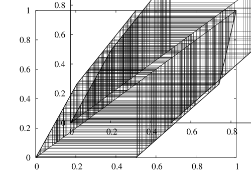
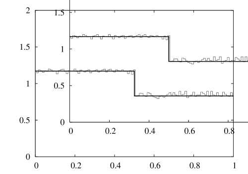
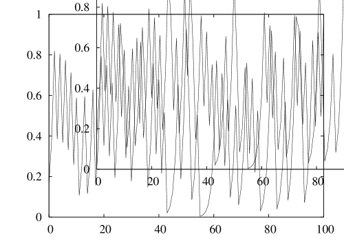
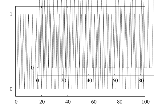
Figure 1: Comparison of the results by the Markov process and the Kalman map for $N=2$. (a) Kalman map corresponding to the Markov process with the transition matrix given in Eq. (25). (b) Comparison of the exact invariant density (thick line) with the approximate invariant density (thin line) in terms of unstable 15-periodic orbits by making use of the formula (19). (c) Chaotic time series generated by the mapping dynamics (Left) in (a) and the state evolution (Right) corresponding to the figure (a). The stochastic evolution is generated by the equivalent Kalman dynamics.

n	exact	approximate
0	0.2425	0.2335
1	-0.1027	-0.0984
2	0.0421	0.0434
3	-0.0193	-0.0173
4	0.0097	0.0078
5	-0.0044	-0.0041
6	0.0025	0.0019
7	0.0003	-0.0004
8	0.0000	0.0000

Table 1: Comparison of the exact time correlation function $C_{n}$ from the formula (15) with the approximate one by the Markov method with $M=0$ for $N=2$. The long time average for the latter was replaced by the ensemble average with unstable periodic orbits. See Eq. (19) and Fig. 1(b).

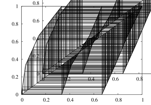
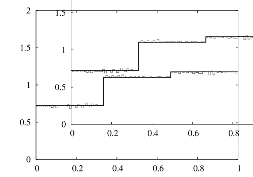
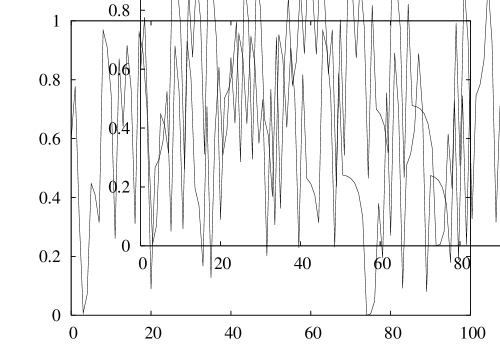
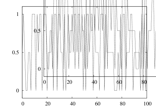
Figure 2: Comparison of the results by the Markov process and the Kalman map for $N=3$. (a) Kalman map corresponding to the Markov process with the transition matrix given in Eq. (25). (b) Comparison of the exact invariant density (thick line) with the approximate invariant density (thin line) in terms of unstable 15-periodic orbits by making use of the formula (19). (c) Chaotic time series generated by the mapping dynamics (Left) in (a) and the state evolution (Right) corresponding to the figure (a). The stochastic evolution is generated by the equivalent Kalman dynamics.

n	exact	approximate
0	0.1538	0.1538
1	-0.0327	-0.0321
2	0.0085	0.0093
3	-0.0028	-0.0021
4	0.0007	-0.0004
5	-0.008	-0.0003
6	0.0006	0.0001
7	0.0000	0.0000
8	0.0000	0.0000

Table 2: Comparison of the exact time correlation function $C_{n}$ from the formula (15) with approximate one by the Markov method with $M=1$ for $N=3$. The long time average for the latter was replaced by the ensemble average with unstable periodic orbits. See Eq. (19) and Fig. 2(b).

IV Concluding remarks and Discussions

In the present paper, we showed that the large deviation deviation statistical quantities of a discrete time, finite state Markov process precisely coincides with that obtained by the Kalman map corresponding to the Markov process. The chaotic dynamics is self-generated and has an inner dynamics. In this sense, although the Kalman dynamics generates the stochastic process under consideration, two dynamics are different. Nevertheless, if one observes the dynamics of the coarse-grained variable, namely the variable $u(x)$ being independent of $x$ if $\beta_{(j-1)N}<x\leq\beta_{jN}$ for each label $j$, provided one cannot distinguish the dynamics of the chaotic dynamics and the stochastic dynamics, then two dynamics give rigorously same results on statistical quantities, i.e., the invariant probability, double-time correlation functions and the large deviation statistical quantities.

Differences between the stochastic process and the Kalman dynamics are caused by the fact that the chaotic variable $x_{n}$ is continuous in contrast to that the states of the present stochastic process are discrete. Furthermore, the Lyapunov exponent is determined for the chaotic dynamics, while it cannot be determined for the stochastic process. The Lyapunov exponent $\lambda=\langle\ln|f^{\prime}(x)|\rangle=\int\rho(x)\ln|f^{\prime}(x)|dx$ for the Kalman map is easily calculated as

$$\lambda=\sum_{j=1}^{N}P_{*}^{(j)}\sum_{k=1}^{N}H_{kj}\ln H_{kj}^{-1}.$$ (26)

Although the Lyapunov exponent is the key concept of chaotic system and cannot be defined in a stochastic process in a conventional sense, the Lyapunov exponent of the Kalman dynamics is fully determined by the quantities contained in the stochastic process. In this sense, the quantity (26) can be called the Lyapunov exponent of the stochastic process (1). One can conclude that the origins of the unpredictability in the finite-state Markov stochastic process and the Kalman dynamics, more exactly speaking, the chaotic dynamics are same. It is worth while to note that Eq. (26) is identical to the equality between the Lyapunov exponent and the Kolmogorov-Sinai entropy of one-dimensional map O93 ; B65 ; CFS82 .

Since a Markov stochastic process can be generated by the Kalman map, statistical quantities of the stochastic process are determined by the chaotic dynamics. By making use of simple examples, we showed that dynamical quantities of the stochastic process can be well approximated in terms of unstable periodic orbits of the Kalman dynamics in Sec. III.

Recently, statistical quantities of the turbulence can be approximated with an admissible unstable periodic orbit KK01 . Furthermore the time correlation function of chaotic dynamics can be well approximated with an appropriate unstable periodic orbit embedded in the attractor KF06 . In the case of Kalman dynamics, we showed in Appendix D that the approximation of time correlations with an appropriate unstable periodic orbit is well done. It is found that the admissible unstable periodic orbit have a passing rate which is similar to the invariant density of the Kalman map.

In closing the paper, let us discuss the applicability of Kalman dynamics to more general stochastic processes. As discussed in the present paper, the Kalman map precisely explains the statistics of finite state discrete time Markov process. However, the Kalman map is a quite special type of mapping dynamics even the dynamics is restricted in mapping system in the sense that the Kalman map is piecewise linear and everywhere hyperbolic. In physical systems observed in experiments, mapping dynamics are usually neither piecewise nor everywhere hyperbolic. This fact implies that physically observed stochastic processes generically cannot be described by finite-state Markov stochastic process. It is quite interesting and important to study the possibility to construct a chaotic dynamics which describe more complicated stochastic dynamics such as continuous state and continuous time stochastic process.

Appendix A Kalman Maps for two and three state processes

In this appendix, examples of the Kalaman map are shown for $N=2$ and 3. One should note that the dynamics $x_{n+1}=f(x_{n})$ with the mapping function (12) shows a chaotic behavior since the local expansion rate $\ln|f^{\prime}(x)|$ of the mapping function is everywhere positive. Therefore, the mapping system (12) turns out to be hyperbolic.

Let us first consider the two-state stochastic process. The positions $\beta_{\underline{j}}\ (\underline{j}=1,2,3)$ are obtained as

$$\beta_{1}=\frac{H_{11}}{2},\ \beta_{2}=\frac{1}{2},\ \beta_{3}=\frac{1}{2}(1+H_{12}).$$ (27)

The mapping function of the Kalman map corresponding to the above is given by

$$f(x)=\begin{cases}H_{11}^{-1}x&\text{($0<x\leq\beta_{1}$)},\\ \beta_{2}+H_{21}^{-1}(x-\beta_{1})&\text{($\beta_{1}<x\leq\beta_{2}$)},\\ H_{12}^{-1}(x-\beta_{2})&\text{($\beta_{2}<x\leq\beta_{3}$)},\\ \beta_{2}+H_{22}^{-1}(x-\beta_{3})&\text{($\beta_{3}<x\leq 1$)}.\end{cases}$$ (28)

The above function is drawn in Fig. 3.

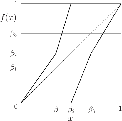
Figure 3: Kalman map constructed from the two-state stochastic process. The positions $\beta_{\underline{j}}$’s are given in Eq. (A1).

For the three-state stochastic process, the positions $\beta_{\underline{j}}\ (\underline{j}=1,2,\cdots,8)$ are obtained as

$$\beta_{1} = \frac{H_{11}}{3},\ \beta_{2}=\frac{1}{3}(H_{11}+H_{21}),\ \beta_{3}=\frac{1}{3},$$

$$\beta_{4} = \frac{1}{3}(1+H_{12}),\ \beta_{5}=\frac{1}{3}(1+H_{12}+H_{22}),\ \beta_{6}=\frac{2}{3},$$

$$\beta_{7} = \frac{1}{3}(2+H_{13}),\ \beta_{8}=\frac{1}{3}(2+H_{13}+H_{23}).$$

(29)

The mapping function of the constructed one-dimensional map is given by

$$f(x)=\begin{cases}H_{11}^{-1}x&\text{($0<x\leq\beta_{1}$)},\\ \beta_{3}+H_{21}^{-1}(x-\beta_{1})&\text{($\beta_{1}<x\leq\beta_{2}$)},\\ \beta_{6}+H_{31}^{-1}(x-\beta_{2})&\text{($\beta_{2}<x\leq\beta_{3}$)},\\ H_{12}^{-1}(x-\beta_{3})&\text{($\beta_{3}<x\leq\beta_{4}$)},\\ \beta_{3}+H_{22}^{-1}(x-\beta_{4})&\text{($\beta_{4}<x\leq\beta_{5}$)},\\ \beta_{6}+H_{32}^{-1}(x-\beta_{5})&\text{($\beta_{5}<x\leq\beta_{6}$)},\\ H_{13}^{-1}(x-\beta_{6})&\text{($\beta_{6}<x\leq\beta_{7}$)},\\ \beta_{3}+H_{23}^{-1}(x-\beta_{7})&\text{($\beta_{7}<x\leq\beta_{8}$)},\\ \beta_{6}+H_{33}^{-1}(x-\beta_{8})&\text{($\beta_{8}<x\leq 1$)}.\end{cases}$$ (30)

The function $f(x)$ is drawn in Fig. 4.

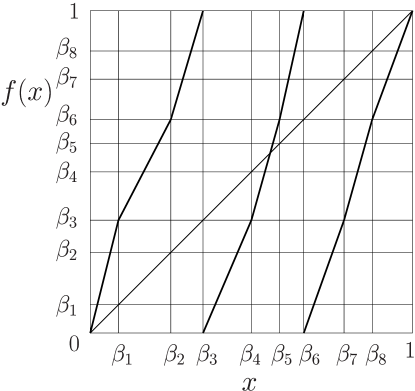
Figure 4: Kalman map constructed from the three-state stochastic process. The positions $\beta_{\underline{j}}$’s are given in Eq. (A3).

Appendix B Proofs of the statements in sec. II

B.1 Invariant probability density

Let us consider the chaotic dynamics $x_{n+1}=f(x_{n})$ with the piecewise linear mapping function (12). The probability density $\rho_{n}(x)$ obeys the evolution equation $\rho_{n+1}(x)={\cal H}\rho_{n}(x)$ with the Frobenius-Perron operator ${\cal H}$. One can show that the invariant density $\rho(x)(={\cal H}\rho(x))$ is expanded as

$$\rho(x)=\sum_{\underline{j}=1}^{N^{2}}\underline{c}_{\underline{j}}\underline{I}_{\underline{j}}(x).$$ (31)

Here the function $\underline{I}_{\underline{j}}(x)$ is defined as

$$\underline{I}_{\underline{j}}(x)=\begin{cases}1&\text{for $\beta_{\underline{j}-1}<x\leq\beta_{\underline{j}}$},\\ 0&\text{otherwise},\end{cases}$$ (32)

$(\underline{j}=1,2,\cdots,N^{2})$. The coefficients $\underline{c}_{1},\underline{c}_{2},\cdots,\underline{c}_{N^{2}}$ are determined as follows. First, note the relation

$${\cal H}\underline{I}_{\underline{j}}(x)=\sum_{\mu}\frac{\underline{I}_{\underline{j}}(y_{\mu})}{|f^{\prime}(y_{\mu})|}=\sum_{\underline{k}=1}^{N^{2}}\underline{I}_{\underline{k}}(x)\underline{H}_{\underline{k}\underline{j}},$$ (33)

where $\underline{H}_{\underline{k}\underline{j}}$ is the $\underline{k}\underline{j}$ element of an $x$-independent $N^{2}\times N^{2}$ matrix $\hat{\underline{H}}$. The matrix $\hat{\underline{H}}$ is obtained as follows. By putting $\underline{j}=(j-1)N+j^{\prime}\ ,\ \underline{k}=(k-1)N+k^{\prime}$ with $1\leq j\leq N,\ 1\leq k\leq N,\ 1\leq j^{\prime}\leq N$ and $\ 1\leq k^{\prime}\leq N$ and by noting $\underline{I}_{\underline{j}}(y_{\mu})/|f^{\prime}(y_{\mu})|=H_{j^{\prime}j}\underline{I}_{\underline{j}}(y_{\mu})$, Eq. (B3) is written as

$$H_{j^{\prime}j}\sum_{\mu}\underline{I}_{\underline{j}}(y_{\mu})=\sum_{\underline{k}=1}^{N^{2}}\underline{I}_{\underline{k}}(x)\underline{H}_{\underline{k}\underline{j}}.$$ (34)

Multiplying $\underline{I}_{\underline{k}}(x)$ to Eq. (B3) and integrating it over $x$, we obtain

$$\underline{H}_{\underline{k}\underline{j}} = N\frac{H_{j^{\prime}j}}{H_{k^{\prime}k}}\int\underline{I}_{(k-1)N+k^{\prime}}(x)\sum_{\mu}\underline{I}_{(j-1)N+j^{\prime}}(y_{\mu}(x))dx$$ (35)

$$= H_{kj}\delta_{kj^{\prime}},$$

where we gave used $\underline{I}_{(k-1)N+k^{\prime}}(x)\sum_{\mu}\underline{I}_{(j-1)N+j^{\prime}}(y_{\mu}(x))=\delta_{j^{\prime}k}\underline{I}_{(k-1)N+k^{\prime}}(x)$.

The explicit form of the $N^{2}\times N^{2}$ matrix $\hat{\underline{H}}$ is given by

$$\hat{\underline{H}}=\hskip 426.79134pt$$

$$\left(\begin{array}[]{@{\,}ccccc|ccccc|c|ccccc@{\,}}H_{11}&0&\ldots&0&0&H_{12}&0&\ldots&0&0&\ldots&H_{1N}&0&\ldots&0&0\\ H_{11}&0&\ldots&0&0&H_{12}&0&\ldots&0&0&\ldots&H_{1N}&0&\ldots&0&0\\ \vdots&\vdots&\ddots&\vdots&\vdots&\vdots&\vdots&\ddots&\vdots&\vdots&\vdots&\vdots&\vdots&\ddots&\vdots&\vdots\\ H_{11}&0&\ldots&0&0&H_{12}&0&\ldots&0&0&\ldots&H_{1N}&0&\ldots&0&0\\ \hline\cr 0&H_{21}&\ldots&0&0&0&H_{22}&\ldots&0&0&\ldots&0&H_{2N}&\ldots&0&0\\ 0&H_{21}&\ldots&0&0&0&H_{22}&\ldots&0&0&\ldots&0&H_{2N}&\ldots&0&0\\ \vdots&\vdots&\ddots&\vdots&\vdots&\vdots&\vdots&\ddots&\vdots&\vdots&\vdots&\vdots&\vdots&\ddots&\vdots&\vdots\\ 0&H_{21}&\ldots&0&0&0&H_{22}&\ldots&0&0&\ldots&0&H_{2N}&\ldots&0&0\\ \hline\cr&\vdots&&&&&\vdots&&&&\ddots&&\vdots&&&\\ \hline\cr 0&0&\ldots&0&H_{N1}&0&0&\ldots&0&H_{N2}&\ldots&0&0&\ldots&0&H_{NN}\\ 0&0&\ldots&0&H_{N1}&0&0&\ldots&0&H_{N2}&\ldots&0&0&\ldots&0&H_{NN}\\ \vdots&\vdots&\ddots&\vdots&\vdots&\vdots&\vdots&\ddots&\vdots&\vdots&\vdots&\vdots&\vdots&\ddots&\vdots&\vdots\\ 0&0&\ldots&0&H_{N1}&0&0&\ldots&0&H_{N2}&\ldots&0&0&\ldots&0&H_{NN}\end{array}\right).$$ (49)

(50)

With the expression (B1) and the relation (B3), we get

$${\cal H}\rho(x)=\sum_{\underline{j}=1}^{N^{2}}\underline{c}_{\underline{j}}\sum_{\underline{k}=1}^{N^{2}}\underline{I}_{\underline{k}}(x)\underline{H}_{\underline{k}\underline{j}}.$$ (51)

Equating Eqs. (B1) and (B7), one obtains

$$\underline{c}_{\underline{j}}=\sum_{\underline{k}=1}^{N^{2}}\underline{H}_{\underline{j}\underline{k}}\underline{c}_{\underline{k}}.$$ (52)

By noting the relation (B5), Eq. (B8) is rewritten as

$$\underline{c}_{(j-1)N+j^{\prime}}=\sum_{k=1}^{N}H_{jk}\underline{c}_{(k-1)N+j},$$ (53)

where we put $\underline{j}=(j-1)N+j^{\prime}\ ,\ \underline{k}=(k-1)N+k^{\prime},1\leq j\leq N,\ 1\leq k\leq N$ and $\ 1\leq j^{\prime}\leq N,\ 1\leq k^{\prime}\leq N$. Since the r.h.s. of Eq. (B9) is independent of $j^{\prime}$, we find that $\underline{c}_{(j-1)N+j^{\prime}}$ is free from $j^{\prime}$. Therefore, by putting $\underline{c}_{(j-1)N+1}=\underline{c}_{(j-1)N+2}=\underline{c}_{(j-1)N+3}=\cdots=\underline{c}_{(j-1)N+N}\equiv c_{j}$, Eq. (B9) is written as

$$c_{j}=\sum_{k=1}^{N}H_{jk}c_{k},$$ (54)

and the probability density $\rho(x)$ given in Eq. (B1) is rewritten as

$$\rho(x)=\sum_{j=1}^{N}c_{j}I_{j}(x),$$ (55)

where we have defined

$$I_{j}(x)=\begin{cases}1&\text{for $\beta_{(j-1)N}<x\leq\beta_{jN}$},\\ 0&\text{otherwise}.\end{cases}$$ (56)

In order that Eq. (B10) agrees with the result (4) in the stochastic process, we need $c_{j}=\alpha P_{*}^{(j)}$, where $\alpha$ is independent of $j$. Furthermore, noting the normalization condition of the probability density $\rho(x)$, we find $c_{j}=NP_{*}^{(j)}$, $(j=1,2,\cdots,N)$. Equation (B10) thus turns out to be identical with Eq. (4) in the stochastic process.

B.2 Double-time correlation function

The equivalence of the double time correlation functions derived from the Markov process (1) and that from the corresponding Kalman map was recently shown by Kohda and Fujisaki KF99 . The following discussion is the simplified one of their proof. The time correlation function $C_{n}^{\rm K}$ for a function $u(x_{n})$, where $u(x)$ takes the value $a^{(j)}$ if $\beta_{(j-1)N}<x\leq\beta_{jN}$, is rewritten as

$$C_{n}^{\rm K}=\int\delta u(x_{n})\delta u(x)\rho(x)dx.$$ (57)

By defining the quantities $\underline{a}^{(\underline{k})}$’s by $\underline{a}^{(\underline{k})}=a^{(k)}$ for $\underline{k}=(k-1)N+k^{\prime},(1\leq k\leq N,1\leq k^{\prime}\leq N)$ and $\delta\underline{a}^{(\underline{k})}=\underline{a}^{(\underline{k})}-\langle u\rangle$ and inserting the expression (B1) and $\delta u(x)=\sum_{\underline{k}=1}^{N^{2}}\delta\underline{a}^{(\underline{k})}\underline{I}_{\underline{k}}(x)$ into Eq. (B13), one gets

$$C_{n}^{\rm K} = \int\rho(x)\delta u(x){\cal L}^{n}\delta u(x)dx$$ (58)

$$= \int\delta u(x){\cal H}^{n}[\rho(x)\delta u(x)]dx$$

$$= \sum_{\underline{j}=1}^{N^{2}}\sum_{\underline{k}=1}^{N^{2}}\underline{c}_{\underline{j}}\delta\underline{a}^{(\underline{j})}\delta\underline{a}^{(\underline{k})}\int\underline{I}_{\underline{k}}(x){\cal H}^{n}\underline{I}_{\underline{j}}(x)dx,$$

where ${\cal L}$ is the time evolution operator defined by ${\cal L}G(x)=G(f(x))$. By noting

$${\cal H}^{n}\underline{I}_{\underline{j}}(x)=\sum_{\underline{k}=1}^{N^{2}}\underline{I}_{\underline{k}}(x)(\hat{\underline{H}}^{n})_{\underline{k}\underline{j}},$$ (59)

the time correlation function is expanded as

$$C_{n}^{\rm K}=\sum_{\underline{j}=1}^{N^{2}}\sum_{\underline{k}=1}^{N^{2}}\Delta_{\underline{k}}\delta\underline{a}^{(\underline{k})}(\hat{\underline{H}}^{n})_{\underline{k}\underline{j}}\delta\underline{a}^{(\underline{j})}\underline{c}_{\underline{j}},$$ (60)

where $\Delta_{\underline{k}}\equiv\int\underline{I}_{\underline{k}}(x)dx$. Putting $\underline{j}=(j-1)N+j^{\prime}$ and $\underline{k}=(k-1)N+k^{\prime}$ with $1\leq j\leq N,1\leq k\leq N,1\leq j^{\prime}\leq N$ and $1\leq k^{\prime}\leq N$, we get $\Delta_{\underline{k}}=\beta_{(k-1)N+k^{\prime}}-\beta_{(k-1)N+k^{\prime}-1}=H_{k^{\prime}k}/N$, and therefore $\sum_{k^{\prime}=1}^{N}\Delta_{(k-1)N+k^{\prime}}=\beta_{kN}-\beta_{(k-1)N}=N^{-1}$. These relations lead to

$$(\hat{\underline{H}}^{n})_{\underline{k}\underline{j}}=(\hat{H}^{n-1})_{kj^{\prime}}H_{j^{\prime}j},$$ (61)

$(n=1,2,3,\cdots)$. Furthermore, since $\delta\underline{a}^{(\underline{j})}=\delta a^{(j)}$ and $\underline{c}_{\underline{j}}=NP_{*}^{(j)}$, Eq. (B16) is reduced to the time correlation function (5) obtained in the stochastic process.

B.3 Large deviation theoretical characteristic function

The large deviation theoretical characteristic function for the time series $\{u(x_{m})\}$, where $u(x)$ takes the value $a^{(j)}$ if $\beta_{(j-1)N}<x\leq\beta_{jN},(j=1,2,\cdots,N)$. The characteristic function is rewritten as

$$Z^{\rm K}_{q}(n)=\int{\cal H}_{q}^{n}\rho(x)dx,$$ (62)

where ${\cal H}_{q}$ is the generalized (order-$q$) Frobenius-Perron operator ST86 ; FI87b defined as

$${\cal H}_{q}G(x)\equiv{\cal H}\left[e^{qu(x)}G(x)\right]=\sum_{\mu}\frac{e^{qu(y_{\mu})}G(y_{\mu})}{|f^{\prime}(y_{\mu})|}.$$ (63)

Noting the relation

$${\cal H}_{q}\underline{I}_{\underline{j}}(x)=\sum_{\underline{k}=1}^{N^{2}}\underline{I}_{\underline{k}}(x)(\hat{\underline{H}}_{q})_{\underline{k}\underline{j}}$$ (64)

with the matrix $\hat{\underline{H}}_{q}$ whose $\underline{k}\underline{j}$ element is defined by

$$(\hat{\underline{H}}_{q})_{\underline{k}\underline{j}}=\underline{H}_{\underline{k}\underline{j}}\exp[q\underline{a}^{(\underline{j})}],$$ (65)

$(\hat{\underline{H}}_{q=0}=\hat{\underline{H}})$, one obtains

$${\cal H}_{q}^{n}\underline{I}_{\underline{j}}(x)=\sum_{\underline{k}}\underline{I}_{\underline{k}}(x)(\hat{\underline{H}}_{q}^{n})_{\underline{k}\underline{j}}.$$ (66)

Therefore, since ${\cal H}_{q}^{n}\rho(x)=\sum_{\underline{j}}\sum_{\underline{k}}\underline{c}_{\underline{j}}\underline{I}_{\underline{k}}(x)(\hat{\underline{H}}_{q}^{n})_{\underline{k}\underline{j}}$, we obtain $Z_{q}^{\rm K}(n)=\sum_{\underline{j}}\sum_{\underline{k}}\underline{c}_{\underline{j}}\Delta_{\underline{k}}(\hat{\underline{H}}_{q}^{n})_{\underline{k}\underline{j}}$ If we put $\underline{j}=(j-1)N+j^{\prime},\underline{k}=(k-1)N+k^{\prime}$ with $1\leq j\leq N,1\leq j^{\prime}\leq N,1\leq k\leq N$ and $1\leq k^{\prime}\leq N$, then noting $\underline{c}_{\underline{j}}=c_{j},\Delta_{\underline{k}}=H_{k^{\prime}k}/N$ and

$$(\hat{\underline{H}}_{q})_{\underline{k}\underline{j}} = (\hat{H}_{q})_{kj}\delta_{kj^{\prime}},$$ (67)

$$(\hat{\underline{H}}_{q}^{n})_{\underline{k}\underline{j}} = (\hat{H}_{q}^{n-1})_{kj^{\prime}}(\hat{H}_{q})_{j^{\prime}j},$$ (68)

where $(\hat{H}_{q})_{kj}=H_{kj}e^{qa^{(j)}}$, we obtain $Z_{q}^{\rm K}(n)=\sum_{j}\sum_{k}(\hat{H}_{q}^{n})_{kj}\frac{c_{j}}{N}$. By making use of $c_{j}=NP_{*}^{(j)}$, the above expression coincides with Eq. (9).

As proved above, those of the present chaotic dynamics constructed in the preceding section gives the results precisely same as those of the stochastic process. Therefore, the one-dimensional chaotic dynamics with the mapping function (12) precisely simulates the stochastic process (1).

Appendix C Markov method for time correlation functions of one-dimensional map

We consider a chaotic one-dimensional map,

$$x_{n+1}=f(x_{n}),$$ (69)

($n=0,1,2,\cdots)$. The time series $\{u_{n}\}$ under consideration is given by $u_{n}=h\{x_{n}\}$, where $h\{x\}$ is a unique scalar function of $x$. In terms of the time evolution operator $\mathcal{L}$ defined by $\mathcal{L}G(x)=G(f(x))$, $u_{n}$ obeys the equation of motion $u_{n+1}=\mathcal{L}u_{n}$. The time correlation function $C_{n}=\langle u_{n}u_{0}\rangle$, where $\langle\cdots\rangle$ denotes the long time average, with $u_{n}$ being chosen such that $\langle u_{n}\rangle=0$, can be obtained by the Markov method proposed in Ref. F05 as follows.

First, we introduce the vector variable

$${\mbox{\boldmath{$u$}}}\{x\}\equiv(h_{1}\{x\},h_{2}\{x\},\cdots,h_{M+1}\{x\})^{T},$$ (70)

where $h_{1}\{x\}$ is identical to $h\{x\}$ under consideration. $M$ is the number of new scalar variables, $h_{2},h_{3},\cdots,h_{M+1}$, and is assumed to be suitably chosen. The functions $h_{1},h_{2},\cdots,h_{M+1}$ are chosen so as to have vanishing means and have components linearly independent of each other. The vector variable ${\mbox{\boldmath{$u$}}}_{n}$ defined by

$${\mbox{\boldmath{$u$}}}_{n}=\mathcal{L}^{n}{\mbox{\boldmath{$u$}}}_{0},\ \ \ {\mbox{\boldmath{$u$}}}_{0}={\mbox{\boldmath{$u$}}}\{x\},$$ (71)

obeys the equation of motion ${\mbox{\boldmath{$u$}}}_{n+1}=\mathcal{L}{\mbox{\boldmath{$u$}}}_{n}$.

With the projection operator method FY78 , the above equation can be written in the form of the Mori equation of motion with a memory term. If $M$ is appropriately chosen, the contribution from the memory term is expected to be small and can be ignored F05 . With this approximation, the Mori equation reduces to

$${\mbox{\boldmath{$u$}}}_{n+1}\approx\hat{\zeta}{\mbox{\boldmath{$u$}}}_{n}+{\mbox{\boldmath{$g$}}}_{n}$$ (72)

with

$$\hat{\zeta}\equiv\langle[\mathcal{L}{\mbox{\boldmath{$u$}}}_{0}]{\mbox{\boldmath{$u$}}}^{T}_{0}\rangle\langle{\mbox{\boldmath{$u$}}}_{0}{\mbox{\boldmath{$u$}}}^{T}_{0}\rangle^{-1}.$$ (73)

The fluctuating force ${\mbox{\boldmath{$g$}}}_{n}$ is orthogonal to ${\mbox{\boldmath{$u$}}}_{0}$, i.e., $\langle{\mbox{\boldmath{$g$}}}_{n}{\mbox{\boldmath{$u$}}}_{0}^{T}\rangle=\hat{0},\quad(n\geq 0)$. By noting this property, the time correlation matrix $\hat{C}_{n}\equiv\langle{\mbox{\boldmath{$u$}}}_{n}{\mbox{\boldmath{$u$}}}^{T}_{0}\rangle$ obeys $\hat{C}_{n+1}\approx\hat{\zeta}\hat{C}_{n}$, which yields

$$\hat{C}_{n}\approx\hat{\zeta}^{n}\hat{C}_{0}.$$ (74)

By noting $\hat{\zeta}=\hat{C}_{1}\hat{C}_{0}^{-1}$, the time correlation function $C_{n}$ is thus given by the 1-1 component of $\hat{C}_{n}$. The above approach to the time correlation function is called the Markov method F05 ; KF06 .

Appendix D Determination of time-correlation functions in terms of one unstable periodic orbit

In Sec. III, we determined time correlation functions of the Markov process in terms of many unstable periodic orbits embedded in the corresponding Kalman map. In particular we describe time correlation functions with static quantities ($\hat{C}_{0}$ and $\hat{C}_{1}$) and those static quantities with many unstable periodic orbits. However, for calculation of $\hat{C}_{0}$ and $\hat{C}_{1}$ we do not have to determine the invariant density in terms of so many unstable periodic orbits because $\hat{C}_{0}$ and $\hat{C}_{1}$ include only low order momentums. Here, as the simplest case, we determine dynamical correlations in terms of only single periodic orbit with a passing rate which is similar to invariant density. Thus we use the approximation to determine $\hat{C}_{0}$ and $\hat{C}_{1}$ in terms of an appropriate unstable periodic orbit instead of the long-time average as

$$\langle G(x)\rangle\approx\frac{1}{N_{p}}\sum_{j=0}^{n-1}G(x_{j}^{(p)}),$$ (75)

where $x_{j+N_{p}}^{(p)}=x_{j}^{(p)}$, $(j=1,2,\cdots,N_{p})$ being a period-$N_{p}$ unstable periodic orbit appropriately chosen. If this approximation holds, then the dynamical correlation functions can be approximately expanded in terms of an unstable periodic orbit KF06 .

Hereafter we will compare the time correlation functions with those by periodic orbit for N=2. The transition matrices $\hat{H}$’s for $N=2$ under study is the same as Sec. III.

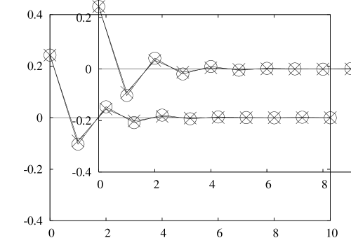
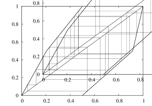
Figure 5: (a) Comparison of the exact time correlation function from the formula (15) ($\circ$) with the approximate one by the Markov method with $M=0$ ($\times$). The long time average for the latter was replaced by the average over the unstable periodic orbit shown in (b). See Eq. (75). (b) The unstable periodic orbit with the period 12.

The results are shown in Fig. (5). Fig. (5) (a) shows the comparison between the time correlation functions obtained with the Markov method ($M=0$) and the unstable periodic orbit shown in (b) with the exact one, Eq. (15). One finds that even if only one unstable periodic orbit is used, one finds that the approximation is well done.

References

- (1) P. Bergé, Y. Pomeau and C. Vidal, Order within Chaos (Wiley, New York, 1984).
- (2) H. G. Schuster and W. Just, Deterministic Chaos - An Introduction -, 4th ed. (Wiley-VCH, Berlin, 2005).
- (3) Y. Ueda, The Road to Chaos (Aerial Press, Santa Cruz, 1992).
- (4) E. Ott, Chaos in Dynamical Systems (Cambridge Univ. Press, Cambridge, 1993).
- (5) H. Mori and Y. Kuramoto, Dissipative Structures and Chaos (Springer-Verlag, Berlin, 1997).
- (6) E. N. Lorenz, J. Atomos. Sci. 20, 130 (1963).
- (7) R. E. Kalman, in Proceedings of the Symposium on Nonlinear Circuit Analysis, New York, N.Y., April 25, 26, 27, 1956”, Ed. J. Fox, (Polytechnic Press, Brooklyn, 1957).
- (8) A. Rényi, Acta Math. Acad. Sci. Hunger. 8, 477 (1957).
- (9) A. Boyarsky and P. Góra, Laws of Chaos: Invariant Measures and Dynamical Systems in One Dimension (Birkh’́auser, Boston, 1997).
- (10) D. J. Driebe, Fully Chaotic Maps and Broken Time Symmetry (Kluwer Academic Publishers, Doordrecht, 1999).
- (11) T. Kohda and H. Fujisaki, IEICE Trans. Fundamentals, E82-A, 1747 (1999), and their papers cited therein.
- (12) R. S. Ellis, Entropy, Large Deviations, and Statistical Mechanics (Springer-Verlag, Berlin, 1985); A. D. Wenzell, Limit Theorems on Large Deviations for Markov Stochastic Processes (Kluwer Academic, Dortrecht and London, 1990).
- (13) H. Fujisaka and M. Inoue, Prog. Theor. Phys. 77, 1334 (1987).
- (14) H. Fujisaka and M. Inoue, Prog. Theor. Phys. 78, 268 (1987).
- (15) H. Fujisaka and M. Inoue, Phys. Rev. A, 39, 1376 (1989); 41, 5302 (1990).
- (16) H. Fujisaka and H. Shibata, Prog. Theor. Phys. 85, 187 (1991).
- (17) H. Fujisaka, in From Phase Transitions to Chaos (Topics in Modern Statistical Physics), ed. G. Györgyi, I. Kondor, L. Sasvári and T. Tél (World-Scientific, Singapore, 1992), 434-448.
- (18) H. Fujisaka, Prog. Theor. Phys. 114, 1 (2005).
- (19) W. Just and H. Fujisaka, Physica D 64, 98 (1993).
- (20) P. Szépfalusy and T. Tél, Phys. Rev. A 34, 2520 (1986).
- (21) H. Fujisaka, H. Shigematsu and B. Eckhardt, Z. Phys. B 92, 235 (1993).
- (22) P. Cvitanović, R. Artuso, P. Dahlqvist, R. Mainieri, G. Tanner, G. Vattay, N. Whelan and A. Wirzba, Chaos: Classical and Quantum (2003), http://www.nbi.dk/ChaosBook/.
- (23) P. Cvitanović, Phys. Rev. Lett. 61, 2729 (1988).
- (24) P. Cvitanović and B. Eckhardt, J. of Phys. A 24, L237 (1991).
- (25) F. Christiansen, G. Paladin and H. H. Rugh, Phys. Rev. Lett. 65, 2087 (1990).
- (26) H. H. Rugh, Nonlinearity 5, 1237 (1992).
- (27) B. Eckhardt, Acta Phys. Polon. B 24, 771 (1993).
- (28) M. U. Kobayashi and H. Fujisaka, Prog. Theor. Phys. 115, 701 (2006).
- (29) C. Grebogi, E. Ott and J.A. Yorke, Phys. Rev. A 37, 1711 (1988).
- (30) T. Morita, H. Hata, H. Mori, T. Horita and K. Tomita, Prog. Theor. Phys. 79, 296 (1988).
- (31) T. Kai and K. Tomita, Prog. Theor. Phys. 64, 1532 (1980).
- (32) P. Billingsley, Ergodic Theory and Information (Wiley, New York, 1965).
- (33) I. Cornfeld, S. Fomin and Ya. G. Sinai, Ergodic Theory (Springer, New York, 1982).
- (34) G. Kawahara and S. Kida, J. Fluid Mech. 449, 291 (2001).
- (35) H. Fujisaka and T. Yamada, Z. Naturforsch. 33a, 1455 (1978).