Percolation of Vortices in the 3D Abelian Lattice Higgs Model

Abstract

The compact Abelian Higgs model is simulated on a cubic lattice where it possesses vortex lines and pointlike magnetic monopoles as topological defects. The focus of this high-precision Monte Carlo study is on the vortex network, which is investigated by means of percolation observables. In the region of the phase diagram where the Higgs and confinement phases are separated by a first-order transition, it is shown that the vortices percolate right at the phase boundary, and that the first-order nature of the transition is reflected by the network. In the crossover region, where the phase boundary ceases to be first order, the vortices are shown to still percolate. In contrast to other observables, the percolation observables show finite-size scaling. The exponents characterizing the critical behavior of the vortices in this region are shown to fall in the random percolation universality class.

, , , and

1 Introduction

The Abelian Higgs model with a compact gauge field formulated on a three-dimensional (3D) lattice possesses an intriguing phase structure [1, 2, 3]. In addition to the Higgs state where the photon acquires a mass, it exhibits a state in which electric charges are confined. The richness of the model, which serves as a toy model for quark confinement, stems from the presence of two types of topological excitations, viz. vortex lines and magnetic monopoles. The latter are point defects in three dimensions which arise because of the compactness of the U(1) gauge group. In the pure 3D compact Abelian gauge theory, monopoles are known to form a plasma that physically causes confinement of electric charges for all values of the inverse gauge coupling $\beta$ [4]. Being the only parameter present, the pure model therefore possesses only a confinement phase. The coupling to the scalar theory preserves this confinement state and gives in addition rise to a Higgs state. For sufficiently small values of the Higgs self-coupling parameter $\lambda$, the two ground states are separated by a first-order transition [5, 6] as sketched in Fig. 1. For $\lambda$ larger than a critical value $\lambda_{\mathrm{c}}$, which depends on the value of the gauge coupling, the two states are no longer separated by a phase boundary across which thermodynamic observables become singular, as was first shown by Fradkin and Shenker [1] in the limit $\lambda\to\infty$ where fluctuations in the amplitude of the Higgs field become completely suppressed. In other words, it is always possible to cross over from one ground state to the other without encountering a thermodynamic singularity. Because of this, the Higgs and confinement states were thought to constitute a single phase, despite profound differences in physical properties.

This conclusion is supported by symmetry arguments [7]. The relevant global symmetry group of the compact 3D Abelian Higgs model (cAHM) is the cyclic group Z_q of $q$ elements, where the integer $q$ denotes the electric charge of the Higgs field. For the doubly charged case ($q=2$), the relevant symmetry group is Z₂, which is in agreement with the known result that the model undergoes a continuous phase transition belonging to the 3D Ising universality class [1, 8]. For $q=1$, this argument excludes a phase transition characterized by a local order parameter in the spirit of Landau because the group $Z_{1}$, which consists of only the unit element, cannot be spontaneously broken. Stated differently, there exist no local order parameter which distinguishes the Higgs from the confinement state.

In Ref. [9], we argued that the phase diagram is more refined than implied by this picture. We conjectured that although analytically connected, the two ground states can be considered as two distinct phases.

\psfrag{c}{confined}\psfrag{h}{Higgs}\psfrag{n}{$0$}\psfrag{k}{$\kappa$}\psfrag{l}{$\lambda$}\psfrag{lc}{$\lambda_{\mathrm{c}}$}\includegraphics[width=281.85034pt]{pictures/PhaseDiag_sketch4.eps}

Figure 1: Sketch of the phase diagram of the Abelian Lattice Higgs Model as a function of the Higgs self-coupling parameter $\lambda$ and the hopping parameter $\kappa$ at fixed inverse gauge coupling $\beta$. For $\lambda<\lambda_{c}$ the transition from the confined to the Higgs phase is of first-order. For $\lambda>\lambda_{c}$ ordinary observables show no singular behavior and signal a crossover between the two ground states indicated by the dark region emanating from the point where the first-order transition line terminates.

The nature of the phase boundary is intimately connected to the distinct physical properties of the Higgs and confinement phase. For the latter phase to confine electric charges, the monopoles must form a plasma. This in turn can only happen when the line tension of the vortex lines, or flux tubes, connecting monopoles and antimonopoles vanishes, so that they are no longer tightly bound in pairs as in the Higgs phase (for typical configuration plots see the snapshots in Fig. 1). Since the vortex line tension is finite in the Higgs phase and zero in the confinement phase, we argued that the phase boundary is uniquely defined by the vanishing of the vortex line tension, irrespective of the order of the phase transition. The confinement mechanism operating in the 3D cAHM is essentially the dual superconductor scenario [10, 11].

In addition to open vortex lines, each having a monopole and an antimonopole at its endpoints, the system also possesses closed vortex lines. These are expected to be characterized by the same line tension as the open lines. Because of the finite line tension, large vortex loops are exponentially suppressed in the Higgs phase. Upon approaching the phase boundary, the line tension becomes smaller so that the vortex network can grow larger and the overall line density increases. Finally, at the phase boundary where the line tension vanishes, vortices can grow arbitrarily large at no energy cost. The phase boundary between the Higgs and confinement phase is therefore expected to be marked by a proliferation of (open and closed) vortex lines, as was first proposed by Einhorn and Savit [12]. The vortices proliferate both in the region where the transition is first-order and in the region where it is not. A line along which geometrical objects proliferate, yet thermodynamic quantities and other local gauge-invariant observables remain nonsingular has become known as a Kertész line [13]. Such a line was first discussed in the context of spin clusters in the 2D Ising model in an applied magnetic field.

The same deconfinement transition driven by the proliferation of vortices with a phase boundary consisting of a first-order line which ends in a critical point and then continues as a Kertész line was originally proposed by Langfeld for the SU(2) counterpart of the Abelian Higgs model defined on a 4D lattice [14]. The relevant vortices, forming surfaces in 4D, are center vortices which carry a flux related to the nontrivial element of the Z₂ center of the SU(2) gauge group. The presence of the Kertész line in this non-Abelian model has been further numerically investigated and confirmed in Ref. [15]. While the concept of a Kertész line was originally introduced in the context of lattice gauge theories in Ref. [16], the interpretation of a deconfinement transition as driven by percolating vortices was previously put forward in the context of the SU(2) lattice Higgs model [17, 18, 19], and the pure SU(2) lattice gauge theory [20, 21, 22].

The purpose of this Monte Carlo study is to investigate the vortex proliferation scenario suggested in Refs. [9, 23] by studying the behavior of the vortex network directly. Because vortices are geometrical objects, their analysis is amenable to the methods developed in percolation theory [24]. We conjectured in Refs. [9, 23] that along the Kertész line, percolation observables have the usual percolation exponents. In addition, we expect that the vortex network displays discontinuous behavior in the region where the phase boundary consists of a first-order transition. For other recent Monte Carlo studies focusing on various aspects of the model see Refs. [25, 26, 27] and references therein.

A similar high-precision Monte Carlo study of the behavior of a vortex network was recently carried out of the 3D XY and the $|\phi|^{4}$ lattice model [28, 29], respectively. The latter model, whose critical temperature on a cubic lattice is known to high precision, corresponds to taking $\beta\to\infty$ in the Higgs model so that the gauge fields become completely ordered. An important observation made in that study was that the overall vortex line density behaves similar to the energy, and the associated susceptibility similar to the specific heat. The vortex percolation threshold estimated through finite-size scaling analysis of the overall line density data was found to be perfectly consistent with the critical temperature. However, estimates based on any of the vortex percolation observables used, while being close to that temperature, never coincided with it within error bars. Possibly, the mismatches are related to the way the vortex networks are traced out, or to the absence of a stochastic element as present in, for example, the Fortuin-Kasteleyn definition of spin clusters in the Potts model [30]. In any case, since we use the same percolation observables and the same (imperfect) rules to trace out vortex networks, we expect to find a similar mismatch, at least in the region where the transition is no longer discontinuous. To remind the reader of these qualifications, we will sometimes refer to the estimated percolation threshold as “apparent percolation threshold”.

The rest of the paper is organized as follows. In the next section, the observables used to investigate the model are introduced. In Sec. 3, the simulation methods as well as the numerical tools used to analyze the data are discussed. In that section, also a new tool to effectively collapse data gathered on lattices of different size is presented. Sections 4 and 5 contain the Monte Carlo results in the vicinity of the phase boundary for the two regions where it consists of a first-order transition and a Kertész line, respectively. In Sec. 6, the dependence of the location of the percolation threshold is investigated as a function of the parameters of the model. Finally, Sec. 7 contains a discussion of the Monte Carlo results and our conclusions.

2 Definitions and Observables

The Abelian lattice Higgs model with compact gauge field at the absolute zero of temperature is defined by the action $S=S_{\mathrm{g}}+S_{\phi}$, with the gauge part

$$S_{\mathrm{g}}=\beta\sum_{x,\mu<\nu}\left[1-\cos\theta_{\mu\nu}(x)\right],$$ (1)

where $\beta$ is the inverse gauge coupling parameter, $\beta=1/aq^{2}$ with $a$ the lattice spacing and $q$ the electric charge of the Higgs field. We exclusively consider the case $q=1$. The doubly charged Higgs field ($q=2$), which has an even richer topological structure than the $q=1$ case, has recently been investigated in Ref. [31], where it was found that the monopoles form chains. The sum in Eq. (1) extends over all lattice sites $x$ and lattice directions $\mu$, and $\theta_{\mu\nu}(x)$ denotes the usual plaquette variable $\theta_{\mu\nu}(x)=\Delta_{\mu}\theta_{\nu}(x)-\Delta_{\nu}\theta_{\mu}(x)$ with the lattice derivative$\Delta_{\nu}\theta_{\mu}(x)\equiv\theta_{\mu}(x+\nu)-\theta_{\mu}(x)$ and the compact link variable $-\pi\leq\theta_{\mu}(x)<\pi$. The matter part $S_{\phi}$ of the lattice action is given by

$$S_{\phi}=-\kappa\sum_{x,\mu}\rho(x)\rho(x+\mu)\cos\left[\Delta_{\mu}\varphi(x)-q\theta_{\mu}(x)\right]+\sum_{x}\left\{\rho^{2}(x)+\lambda\left[\rho^{2}(x)-1\right]^{2}\right\},$$ (2)

where polar coordinates are chosen to represent the complex Higgs field $\phi(x)=\rho(x)\mathrm{e}^{\mathrm{i}\varphi(x)}$, with the compact phase $-\pi\leq\varphi(x)<\pi$. In Eq. (2), $\kappa$ is the hopping parameter, and $\lambda$ the Higgs self-coupling. We study the theory on a cubic lattice, which either is taken to represent a 3D space or spacetime box, depending on whether one of the dimensions of the lattice is interpreted as (Euclidean) time.

In addition to measuring field observables such as the total action or energy $S$, the hopping energy

$$E_{\mathrm{h}}\equiv\frac{1}{L^{3}}\sum_{x,\mu}\rho(x)\rho(x+\mu)\cos\left[\Delta_{\mu}\varphi(x)-q\theta_{\mu}(x)\right],$$ (3)

the square Higgs amplitude, and coslink energy

$$C\equiv-\frac{1}{3L^{3}}\sum_{x,\mu}\cos\left[\Delta_{\mu}\varphi(x)-q\theta_{\mu}(x)\right],$$ (4)

we especially probe for topological excitations. A gauge invariant vortex line segment $j_{\lambda}(x)$ pointing in the $\lambda=1,2,3$ direction is given by

$$j_{\lambda}(x)=\epsilon_{\lambda\mu\nu}\nabla_{\mu}l_{\nu}(x)-n_{\lambda}(x),$$ (5)

where $l_{\mu}(x)$ is the integer-valued field related to the electric current along the links of the lattice via

$$l_{\mu}(x)=\frac{1}{2\pi}\left\{\nabla_{\mu}\varphi(x)-q\theta_{\mu}(x)-[\nabla_{\mu}\varphi(x)-q\theta_{\mu}(x)]_{2\pi}\right\},$$ (6)

and $n_{\lambda}(x)$ measures the multiples of $2\pi$ with which the plaquette variable is shifted away from the interval $[\pi,\pi)$:

$$n_{\lambda}(x)=\frac{1}{2\pi}\epsilon_{\lambda\mu\nu}\left\{\theta_{\mu\nu}(x)-[\theta_{\mu\nu}(x)]_{2\pi}\right\}.$$ (7)

Here, we use the usual modulo operation $[a]_{2\pi}\equiv\alpha-2\pi n$ which subtracts $n$ multiples of $2\pi$ from the variable $\alpha$ such that $[a]_{2\pi}$ takes values in the interval $[\pi,\pi)$. While $l_{\mu}(x)$ measures the quantized vorticity, $n_{\lambda}(x)$ gives the number of elementary Dirac strings piercing the plaquette with its normal pointing in the $\lambda$ direction.

Monopoles are detected by taking the divergence of $j_{\mu}$, $m(x)=\nabla_{\mu}j_{\mu}(x)$, where $m(x)$ takes on integer values only. Using these definitions, we record the vortex line and monopole densities

$$v\equiv\frac{1}{L^{3}}\sum_{x,\mu}\left|j_{\mu}(x)\right|,\quad M\equiv\frac{1}{L^{3}}\sum_{x}m(x).$$ (8)

As already mentioned in the Introduction, in the $|\phi|^{4}$ theory, $v$ behaves similar to the energy and the associated susceptibility similar to the specific heat [29]. A short summary of results for the observables not involving vortices can be found in Ref. [9].

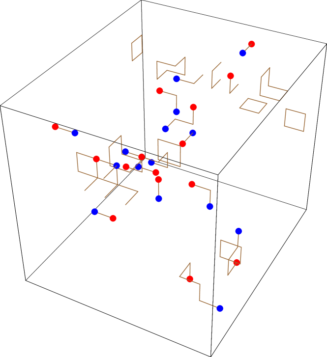
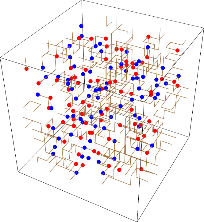
Figure 2: Networks formed by vortex lines. The small spheres represent monopoles and antimonopoles. Left: Higgs phase, characterized by a few short vortex lines which can either be closed or open. Right: Confinement phase, characterized by a large percolating vortex network.

The main focus in this paper is on the vortex networks formed by individual vortex lines (see Fig. 2). Tracing out such a network is ambiguous. We restrict ourselves to the simplest convention by defining a vortex line, which can be either open or closed, as a set of connected vortex line segments. Line segments are said to be connected if they enter or leave the same lattice cube. With this convention, four or six line segments entering and leaving a single cube are not further resolved into separate vortices, but are lumped together into one, self-intersecting vortex. The size $n$ of a vortex is just the number of links forming the vortex. Vortex line segments with $|j_{\mu}|\geq 2$ are not split into distinct segments and are only counted once in the vortex density. The vortex networks found with the help of these tracing rules are therefore only an approximation to the true networks. And the observed, or apparent percolation threshold will in general differ from the true one. We trace out the vortex networks by using a recursive algorithm and employ standard percolation observables to probe them [24]. Specifically, we determine the percolation probability $P_{\mathrm{1D}}$ by recording when a vortex spans the lattice in an arbitrary direction. This definition is such that a vortex is already said to percolate when it spans the lattice in just one, arbitrary direction. We also determine the probability $P_{\mathrm{3D}}$ that a vortex spans the lattice in all directions, and the percolation strength $P_{\infty}$, defined as the size of the largest vortex per lattice site. We have in addition considered the average vortex size, but this data is not well suited for analyses as we also found in previous studies on simpler models [32]. Finally, we use the susceptibility

$$\chi(\mathcal{O})=\left(\langle{\mathcal{O}}^{2}\rangle-\langle{\mathcal{O}}\rangle^{2}\right)L^{3}\,,$$ (9)

(without the $L^{3}$ for $P_{1\mathrm{D}}$ and $P_{3\mathrm{D}}$) and the Binder parameter

$$B(\mathcal{O})=1-\frac{\langle{\mathcal{O}}^{4}\rangle}{3\langle{\mathcal{O}}^{2}\rangle^{2}}$$ (10)

of an observable $\mathcal{O}$ to probe the phase boundary.

3 Simulation and Data Analysis Techniques

3.1 Monte Carlo

A variety of Monte Carlo methods are applied to efficiently simulate the system in the different parts of the phase diagram. In the first-order transition region, primarily the multicanonical algorithm (MUCA) [33] is used with a weight iteration as described in Ref. [34]. Weights are rendered flat in the hopping term (3) of the action to enhance tunnelling. In addition to local updates, the Higgs amplitude and the gauge angles are also updated globally [35] to allow for larger jumps in phase space and thus for shorter tunnelling times between the two metastable states. In the vicinity of the Kertész line, the gauge fields are updated using the Metropolis algorithm, while the Higgs field is updated by means of heat-bath and overrelexation algorithms [36].

Measurements are typically taken after each sweep of the lattice and the entire time series is recorded to allow for error analysis and post-simulation data processing. Table 1 provides an overview of parameters used in the simulations.

Table 1: Number of sweeps of the lattice of linear size $L$ and the number of different values of $\kappa$ considered for each lattice used in the simulations.

$\beta$	$\lambda$	$L$	sweeps	different $\kappa$ values
$1.1$	$0.2$	$10,12,14,16,18,20,22,24,26,30,32,42$	$10^{5}$ – $10^{6}$	20
	$0.75$	$8,10,12,16,20$	$10^{5}$	20
	$0.025$	$8,10,12,14,16,18,20$	$10^{7}$	1 (MUCA)
$2.0$	$0.2$	$8,10,12,14,16,20,24,28,36$	$10^{6}$	10

An integral part of our analysis are Ferrenberg-Swendsen reweighting techniques [37, 38]. These techniques are applied in two distinct flavours. In the Kertész region, we use the multihistogramm reweighting form, which means that we combine simulations at different parameters in an optimal way. Standard reweighting with MUCA weights is applied in the first-order transition region. To apply these techniques in the best possible way we use optimization routines such as the Brent method [39, 40] to search for maxima in susceptibilities or crossing points of Binder parameters. The use of the Jackknife method [41] on top of these methods allows for error estimation of the results so determined.

As an example of this approach, we show in Fig. 3 the susceptibilities of the percolation probability $P_{\mathrm{1D}}$ and the coslink energy $C$. Note that the peak height of $\chi(P_{1\mathrm{D}})$ is exactly $1/4$, since $\langle P_{1\mathrm{D}}^{2}\rangle=\langle P_{1\mathrm{D}}\rangle$ and hence $\chi(P_{1\mathrm{D}})=\langle P_{1\mathrm{D}}\rangle(1-\langle P_{1\mathrm{D}}\rangle)$ is maximal at $\langle P_{1\mathrm{D}}\rangle=1/2$. The points in the plot correspond to individual simulations and the lines through the data points are obtained by reweighting. Different lines in the figure correspond to having different Jackknife blocks (but the same block in each time series) omitted. Notice that the peak in the percolation susceptibility is well defined whereas the peak in the coslink susceptibility is rather broad. The flatness of the peak is reflected in larger error bars on the estimated peak location.

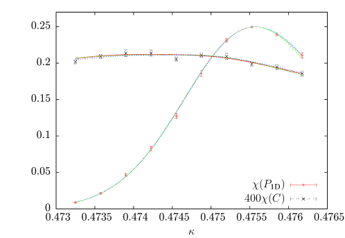
Figure 3: Data points for the susceptibilities $\chi(P_{\mathrm{1D}})$ and $\chi(C)$ (multiplied by $400$) for $\beta=2.0\,,\lambda=0.2$ and different values of $\kappa$ and their interpolating lines obtained through reweighting. The measurements are taken on a cubic lattice of linear size $L=36$.

We have carefully checked our methods against known results for limiting cases such as the London limit $\lambda\to\infty$, where fluctuations in the Higgs amplitude are completely frozen, and the XY model, obtained by setting in addition $\beta=\infty$. A good check whether vortex lines and monopoles are correctly identified is to perform a gauge transformation under which their locations are invariant.

3.2 Finite-size scaling methods

We estimate critical exponents through finite-size scaling analyses. The scaling Ansatz for an observable $\mathcal{O}$ states that in the vicinity of a continuous phase transition, the data obtained for different values of the tuning parameter $\kappa$ and for different lattice sizes $L$ fall onto a (weakly) universal scaling function $f_{\mathcal{O}}$ defined through

$$\mathcal{O}_{L}(\kappa)=L^{\lambda_{\mathcal{O}}/\nu}f_{\mathcal{O}}\left(tL^{1/\nu}\right),\quad t\equiv(\kappa-\kappa_{c})/\kappa_{c}.$$ (11)

Here, $\kappa_{\mathrm{c}}$ denotes the critical point, $\nu$ the correlation length exponent, and $\lambda_{\mathcal{O}}$ is the critical exponent characterizing the observable $\mathcal{O}$. The variable $t$ is the reduced coupling and measures the distance from the critical point.

Data collapse is usually a good check whether the right critical exponents and critical couplings are found by other means. With the correct values, the measured data should fall on the universal curve given by Eq. (11). Here, we reverse this idea. Starting from an initial guess for the critical exponents and couplings, we compute the rescaled observable $\widehat{\mathcal{O}}_{L}(x)=\mathcal{O}_{L}(\kappa)L^{-\lambda_{\mathcal{O}}/\nu}$ with $x=tL^{1/\nu}$ and judge the quality of the collapse in the interval $[x_{\mathrm{min}},x_{\mathrm{max}}]$ by introducing the weight function

$$\sigma^{2}_{\mathcal{O}}\equiv\int_{x_{\mathrm{min}}}^{x_{\mathrm{max}}}\,\mathrm{d}x\left[\overline{\widehat{\mathcal{O}}_{L}^{2}}(x)-\overline{\widehat{\mathcal{O}}_{L}}^{\;2}(x)\right],$$ (12)

with $\overline{\widehat{\mathcal{O}}_{L}}(x)\equiv\sum_{L}\widehat{\mathcal{O}}_{L}(x)/n_{L}$ and $n_{L}$ the number of different lattice sizes included in the sum $\sum_{L}$. A perfect collapse in the window $[x_{\mathrm{min}},x_{\mathrm{max}}]$ would correspond to $\sigma_{\mathcal{O}}^{2}=0$, whereas a bad collapse has a large $\sigma^{2}_{\mathcal{O}}$. This approach qualifies for implementation as an automated method when combined with optimization algorithms to minimize $\sigma^{2}_{\mathcal{O}}$ by adjusting the values of the critical exponents. The method requires that data in each point in the interval $[x_{\mathrm{min}},x_{\mathrm{max}}]$ of the rescaled $x$-axis be compared, most of which has not been measured. A possibility is to interpolate between data points by using a polynomial expansion of the function $f_{\mathcal{O}}$ and to fit its coefficients to the data $\mathcal{O}_{L}$ [42]. The fit then allows for calculating $\sigma_{\mathcal{O}}^{2}$. We use a different approach in that we apply the standard reweighting techniques mentioned above to calculate $\mathcal{O}_{L}$ at every point $\kappa$ and hence $\widehat{\mathcal{O}}_{L}$ at every point $x$. We feel that this approach is more natural and does not add further degrees of freedom to the process.

In practice our implementation is as follows. We first reweight the measured data on all system sizes. We then start with initial values for the exponents and couplings, and apply a minimization algorithm, such as the simplex method [39, 43], that varies the exponents until $\sigma^{2}_{\mathcal{O}}$ is minimized. Since the algorithm can become locked in a local minimum, the procedure must be repeated for many starting points. We find that for our purposes, where only three parameters need to be determined, the routine gives reliable and consistent results. To obtain error estimates, we apply the Jackknife method on top of the whole process. The effect of correction terms to scaling is minimized by repeating the procedure for increasingly smaller intervals $[x_{\mathrm{min}},x_{\mathrm{max}}]$ around the point where collapse is attempted. We expect our tool to be useful in other simulation studies as well. An idea similar to our implementation was recently presented in Ref. [44].

4 First-Order Transition Region

We start our numerical study by investigating the behavior of the vortex network in the first-order transition region of the phase diagram sketched in Fig. 1. We choose to simulate at $\beta=1.1$ and $\lambda=0.025$ where the first-order transition is strong enough already on small lattices so that time consuming simulations on larger systems are not needed.

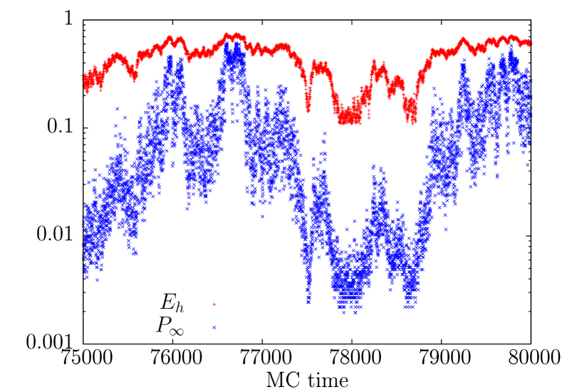
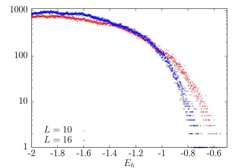
Figure 4: Left: Time series of a MUCA simulation showing the hopping energy $E_{\mathrm{h}}$ (upper curve) and percolation strength $P_{\infty}$ (lower data points) for $L=16$. The two observables are seen to be intimately connected. To fit in one plot, the hopping energy is shifted upwards. Right: Correlation histogram of the number of configurations without a percolating network over hopping energy $E_{\mathrm{h}}$ for system sizes $L=10$ and $16$. Note the logarithmic scale used on the vertical axis.

The left plot in Fig. 4 shows time series of the hopping energy $E_{\mathrm{h}}$ and the percolation strength normalized by the volume as measured in a typical MUCA simulation [33]. Changes in the energy, which reflect the more or less random walk through the metastable region, are seen to occur jointly with changes in the percolation strength. The right plot shows the correlation histogram of the number of configurations without a percolating network versus hopping energy $E_{\mathrm{h}}$. Larger negative energies are seen to strongly correlate with the absence of a percolating vortex network while smaller negative energies strongly correlate with the presence of such a network.

The central thesis we put forward in Ref. [9] is that the phase diagram of the model can be understood in terms of proliferating vortices. In the first-order region, the location of the phase transition has been determined to high precision with the help of observables not involving vortices such as the hopping energy. To determine the location of the percolation threshold in the infinite-volume limit, we consider the vortex percolation probability $P_{\mathrm{1D}}$ and percolation strength $P_{\infty}$, and analyze the scaling of the locations $\kappa_{\mathrm{per}}(L)$ of the maxima in the associated susceptibilities and Binder parameters with lattice size $L$. At a first-order transition, $\kappa_{\mathrm{per}}(L)$ is expected to scale as

$$\kappa_{\mathrm{per}}(L)=\kappa_{\mathrm{per}}+cL^{-3}+\mathcal{O}\left(L^{-6}\right),$$ (13)

with $c$ a constant. We reweight the MUCA time series to obtain the susceptibilities and Binder parameters in the vicinity of $\kappa_{\mathrm{per}}(L)$, and use the methods presented above to search for the peak locations and its error bars.

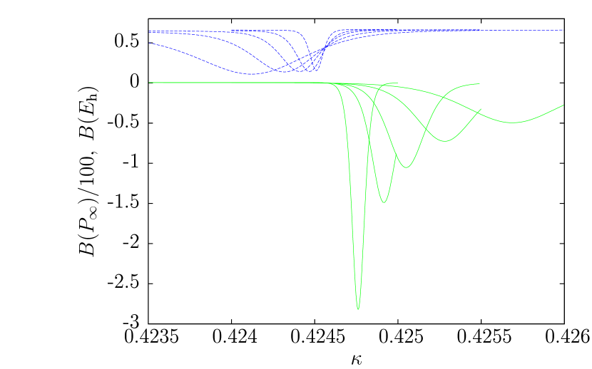
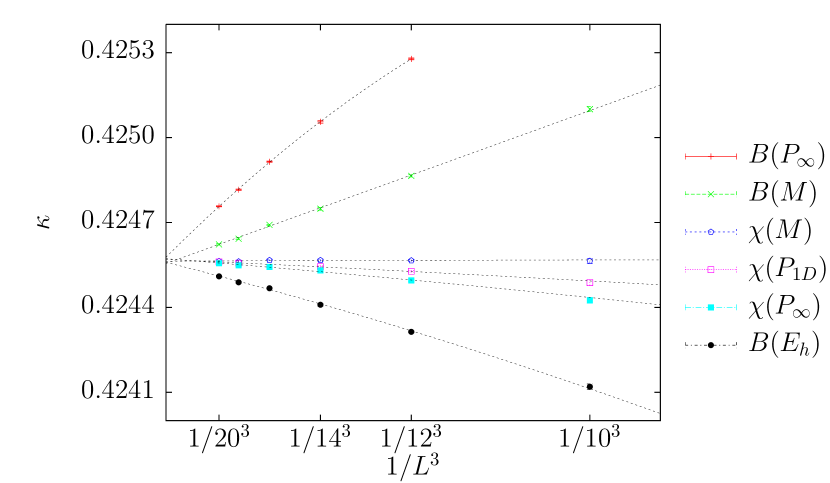
Figure 5: Left: Binder parameters $B(E_{\mathrm{h}})$ (upper curves) and $B(P_{\infty})$ (lower curves) as a function of $\kappa$ in the first-order transition region at $\beta=1.1$, $\lambda=0.025$ measured on lattices of linear size $L=10,12,14,16,20$ (from broad to sharp peaks). The Binder parameter $B(P_{\infty})$ has been divided by 100 so that both parameters fit into one plot. Right: Scaling plots of the maxima of the various Binder parameters and susceptibilities. The Binder parameters show larger finite-size corrections. All curves converge within error bars to the same infinite-volume value of $\kappa_{\mathrm{per}}=\kappa_{\mathrm{c}}=0.424570(3)$.

Figure 5 summarizes our results. It shows the scaling of the percolation thresholds $\kappa_{\mathrm{per}}(L)$ obtained from the percolation probability $P_{\mathrm{1D}}$ and the percolation strength $P_{\infty}$ together with the critical points $\kappa_{\mathrm{c}}(L)$ obtained from the hopping energy $E_{\mathrm{h}}$ and the monopole density $M$. The $\kappa_{\mathrm{per}}(L)$’s obtained from the network observables are seen to strongly depend on the system size, while the $\kappa_{\mathrm{c}}(L)$’s obtained from $\chi(M)$ are almost independent of volume. The results for $\chi(E_{\mathrm{h}})$ are not included in Fig. 5 as they cannot be distinguished from those for $M$ on the scale of the figure. For lattice sizes larger than $L=12$, all curves converge to the same point within error bars. This brings us to the important conclusion that the vortex percolation threshold is located precisely at the first-order transition point. Our best estimate for the transition point, based on both percolation and nonpercolation observables, is $\kappa_{\mathrm{c}}=0.424570(3)$ which is determined from the average of the fit results summarized in Table 2. Averaging the estimates for percolation and non-percolation observables separately, we obtain $\kappa_{\mathrm{per}}=0.424572(4)$ and $\kappa_{\mathrm{c}}=0.424565(4)$, respectively. The absence of a mismatch between the critical temperature and the vortex percolation threshold, as was found in the $|\phi|^{4}$ theory using the same percolation observables [29], is probably because the phase transition is discontinuous here. An abrupt change in the ground state apparently washes out any inaccuracy caused by an imperfect tracing out of the vortex network.

Table 2: Results of fitting the data in Fig. 5 to Eq. (13). The fits starting at $L=8$ and $L=10$ also include the correction term $1/L^{6}$. Those starting at $L=12$ include only the leading term $1/L^{3}$, except for $B(P_{\infty})$, where the correction term is still needed to obtain reasonable results. The number in square brackets denotes $\chi^{2}$ per degree of freedom (DOF), $\chi^{2}/\mathrm{DOF}$. Results are grouped according to percolation and non-percolation observables.

Observable	$L\geq 8$	$L\geq 10$	$L\geq 12$
$\chi(P_{\mathrm{1D}})$	$0.424569(5)$ $[1.6]$	$0.424569(5)$ $[2.0]$	$0.424570(6)$ $[2.3]$
$\chi(P_{\infty})$	$0.424572(6)$ $[1.9]$	$0.424572(5)$ $[2.2]$	$0.424573(6)$ $[2.5]$
$B(P_{\infty})$	$0.424608(10)$ $[10.7]$	$0.424608(10)$ $[13.1]$	$0.424577(6)$ $[1.1]$
$\chi(M)$	$0.424567(3)$ $[2.4]$	$0.424566(5)$ $[3.1]$	$0.424567(6)$ $[4.2]$
$\chi(E_{\mathrm{h}})$	$0.424564(5)$ $[2.52]$	$0.424564(6)$ $[3.1]$	$0.424564(6)$ $[3.2]$
$B(M)$	$0.424558(5)$ $[2.6]$	$0.424558(8)$ $[3.5]$	$0.424555(5)$ $[3.2]$
$B(E_{\mathrm{h}})$	$0.424565(6)$ $[3.3]$	$0.424568(5)$ $[3.9]$	$0.424566(6)$ $[4.0]$

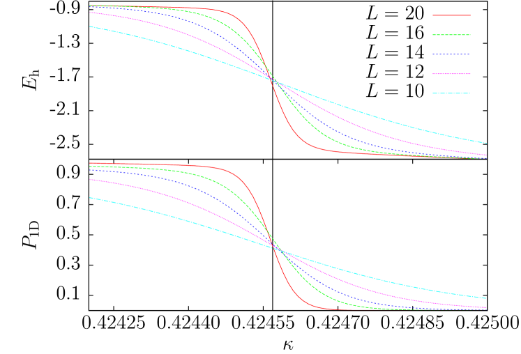
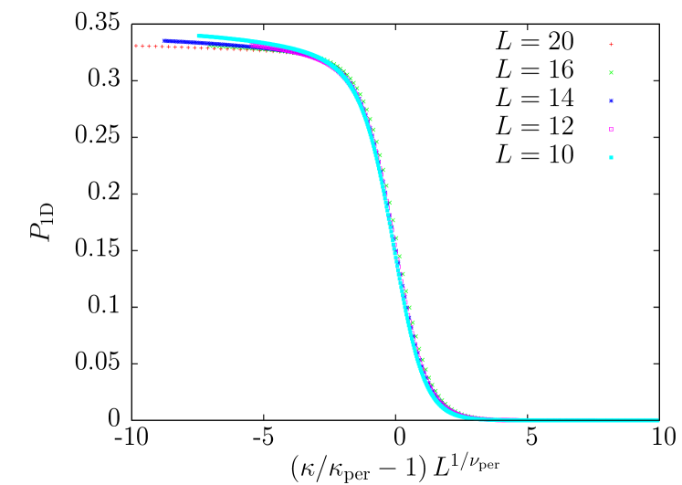
Figure 6: Left: Reweighted hopping energy $E_{\mathrm{h}}$ and percolation probability $P_{\mathrm{1D}}$ for various lattice sizes as a function of the hopping parameter close to the first-order phase transition. The crossing points should provide a second method to estimate the transition point. The estimates obtained using the two observables agree within error bars. Right: Collapse of the $P_{\mathrm{1D}}$ data with $\kappa_{\mathrm{per}}=0.424568,\nu_{\mathrm{per}}=0.325$. An optimal collapse of the $E_{\mathrm{h}}$ data (not shown) is achieved for $\kappa_{\mathrm{c}}=0.424563$ and $\nu=0.338$.

To establish in an unbiased fashion that the vortex network reflects the first-order nature of the transition at $\beta=1.1$ and $\lambda=0.025$, we assume nothing about the transition and apply standard finite-size scaling to the vortex percolation probability $P_{\mathrm{1D}}$ as for a continuous transition. According to Eq. (13), we then expect to find $\nu_{\mathrm{per}}=1/d=1/3$. To obtain an estimate for the percolation threshold $\kappa_{\mathrm{per}}$ on the infinite lattice and $\nu_{\mathrm{per}}$, we reweight the data points from the MUCA time series and subsequently apply our collapsing routine with $\kappa_{\mathrm{per}}$ and $\nu_{\mathrm{per}}$ as free parameters. Figure 6 shows the input and the result of this procedure. The extracted values, $\kappa_{\mathrm{per}}=0.424568(6),\nu_{\mathrm{per}}=0.325(10)$, are perfectly consistent with a first-order transition precisely at the expected location. For comparison, Fig. 6 also shows the hopping energy which is seen to display the same behavior as the percolation probability. Repeating this procedure for the hopping energy data, we obtain $\kappa_{\mathrm{c}}=0.424563(6)$ and $\nu=0.338(10)$. Both these estimates based on the data collapse analysis are perfectly consistent with the previous estimates from finite-size scaling. The raw data in Fig. 6 suggest as in [45] that the crossing points of the curves measured on lattices of different size provide a second method to estimate the transition point.

5 Kertész Line

We continue our analysis of the vortex network in the region where the transition ceases to be of first order. In Ref. [9], we postulated that in this part of the phase diagram the Higgs and confinement phases are separated by a Kertész line. Along this line vortices proliferate, yet thermodynamic quantities remain nonsingular across it. The conjecture is based on the numerical observation that in the Higgs phase, the monopoles are tightly bound in monopole-antimonopole pairs. The magnetic flux emanating from a monopole is squeezed into a magnetic flux tube (vortex) which ends on an antimonopole. The finite line tension forces the vortex lines to be short. In the confinement phase, the monopoles are no longer bound in pairs, but form a plasma. For this to arise, the vortex line tension must vanish. Vortex lines, both open and closed, can then grow arbitrarily long at no energy cost and proliferate.

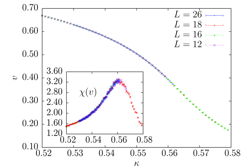
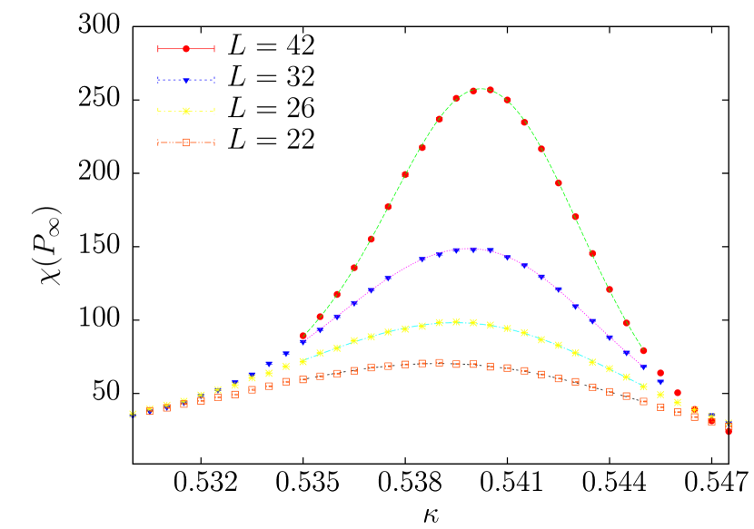
Figure 7: Left: Vortex line density and susceptibility (inset) as a function of the hopping parameter $\kappa$ for systems of linear size $L=12,16,18,26$, and $\beta=1.1\,,\lambda=0.2$. Right: The susceptibility $\chi(P_{\infty})$ as a function of the hopping parameter $\kappa$ for systems of linear size $L=22,26,32,42$.

To facilitate comparison with our previous work [9], we choose the parameters $\beta=1.1$ and $\lambda=0.2$. Figure 7 (left) shows our results for the vortex line density as a function of the hopping parameter $\kappa$ for lattices of linear size varying from $L=12$ to $L=26$. The inset gives the corresponding susceptibilities, which display the same remarkable behavior first observed in the London limit $\lambda\to\infty$ for other observables [8, 25]. Namely, the susceptibility data obtained on lattices of different sizes is seen to collapse without rescaling. In particular, the maxima of the susceptibilities do not show any finite-size scaling. From these data we obtain the estimate $\kappa_{\times}=0.5615(7)$ for the location of the phase boundary. Applying the same analysis to the hopping energy, we arrive at the estimate $\kappa_{\times}=0.5655(7)$ which is close, but does not agree within error bars with the previous estimate. To further investigate this issue, we consider the monopole density to see if it leads to the same estimate as does the hopping energy. The results of our initial study [9] indicated that both estimates agree within error bars. However, the high-precision Monte Carlo simulations carried out in the present work show that this is not the case for the monopole density yields $\kappa_{\times}=0.5639(1)$. In evaluating these results, it should be kept in mind that none of these susceptibilities diverge in the infinite-volume limit, so that small discrepancies were to be expected. The change in the ground state is for this reason usually referred to as a crossover ($\times$). The discrepancy between the peak locations of these observables is shown below in Fig. 9.

In Ref. [9], we argued that the phase diagram is more refined than just showing a crossover between the Higgs and confinement ground states in that a sharp boundary between the two phases does exist in the form of a Kertész line across which the vortices proliferate. Moreover, as we argued partly on the basis of symmetry, the percolation observables in the vicinity of the Kertész line should be characterized by the usual percolation exponents. Unlike the observables previously studied, these observables are expected to show finite-size scaling. Figure 7 (right) shows the susceptibility $\chi(P_{\infty})$ of the percolation strength as a function of the hopping parameter $\kappa$ for lattices of linear size varying from $L=22$ to $L=42$. It is indeed observed that this percolation observable depends on the lattice size even though we considered system sizes larger than those for which the other observables already reached the infinite-volume limit. That is, in contrast to the other observables, percolation observables allow for a precise location of the phase boundary.

To estimate the percolation exponents, we study the behavior of the percolation probability $P_{\mathrm{1D}}$ and $P_{\mathrm{3D}}$ as well as the percolation strength $P_{\infty}$ in the vicinity of the percolation threshold $\kappa_{\mathrm{per}}$ (see Fig. 8). On the infinite lattice, the percolation strength vanishes on approaching the threshold as $P_{\infty}\sim(\kappa-\kappa_{\mathrm{per}})^{\beta_{\mathrm{per}}}$, while $\chi(P_{\infty})$ diverges as $\chi(P_{\infty})\sim|\kappa-\kappa_{\mathrm{per}}|^{-\gamma_{\mathrm{per}}}$. Finally, the correlation length $\xi_{\mathrm{per}}$, which provides a typical length scale of the vortex network, diverges as $\xi_{\mathrm{per}}\sim|\kappa-\kappa_{\mathrm{per}}|^{-\nu_{\mathrm{per}}}$.

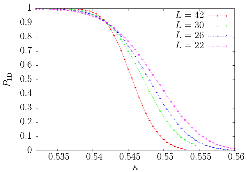
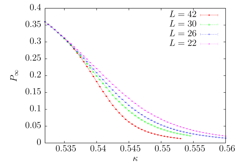
Figure 8: Percolation probability $P_{\mathrm{1D}}$ and percolation strength $P_{\infty}$ as a function of the hopping parameter $\kappa$ for systems of linear size $L=22,26,30,42$ at $\beta=1.1,\,\lambda=0.2$.

Given the discrepancy found in the context of the $|\phi|^{4}$ theory, we do not expect the estimate of the percolation threshold using percolation observables to coincide with the one based on the vortex line density. We therefore determine the location of the percolation threshold anew together with the exponent $\nu_{\mathrm{per}}$ by studying the finite-size behavior of the susceptibilities of percolation observables. Figure 9 shows the scaling of the locations of the susceptibility maxima with $1/L$. The observables considered are the percolation probabilities $P_{\mathrm{1D}}$ and $P_{\mathrm{3D}}$, and the percolation strength $P_{\infty}$. For comparison, also the data for the hopping energy, which was used in Ref. [9] to estimate the location of the phase boundary, and the data for the monopole and vortex densities are included.

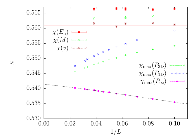
Figure 9: Locations of the susceptibility maxima of the percolation probabilities $P_{\mathrm{1D}}$ and $P_{\mathrm{3D}}$, and the percolation strength $P_{\infty}$ as a function of $1/L$ for $\beta=1.1$. The dashed line is a fit of $\chi_{\mathrm{max}}(P_{\infty})$ to Eq. (14). The horizontal line is through the corresponding data for the vortex density, while the two sets of data points above this line pertain to the monopole density and hopping energy.

The percolation data in Fig. 9 are fitted to the function

$$\kappa_{\mathrm{per}}(L)=\kappa_{\mathrm{per}}+cL^{-1/\nu_{\mathrm{per}}},$$ (14)

using the standard least-squares method. Unfortunately, this approach does not give reliable and consistent values for $\kappa_{\mathrm{per}}$ and $\nu_{\mathrm{per}}$ when repeated for the different observables and lattice sizes. The most stable results are obtained from the susceptibility of $P_{\infty}$, giving $\kappa_{\mathrm{per}}=0.54141(18)$ and $\nu_{\mathrm{per}}=0.87(6)$. Results for $P_{\mathrm{1D}}$ and $P_{\mathrm{3D}}$ depend too much on the fitting regime and we conclude that Eq. (14) for these observables is only fulfilled for large lattice sizes. As expected, the estimate of the location of the percolation threshold does not agree with $\kappa_{\times}$ obtained from the vortex line density.

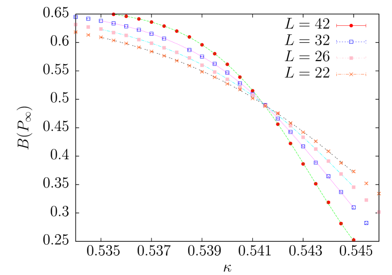
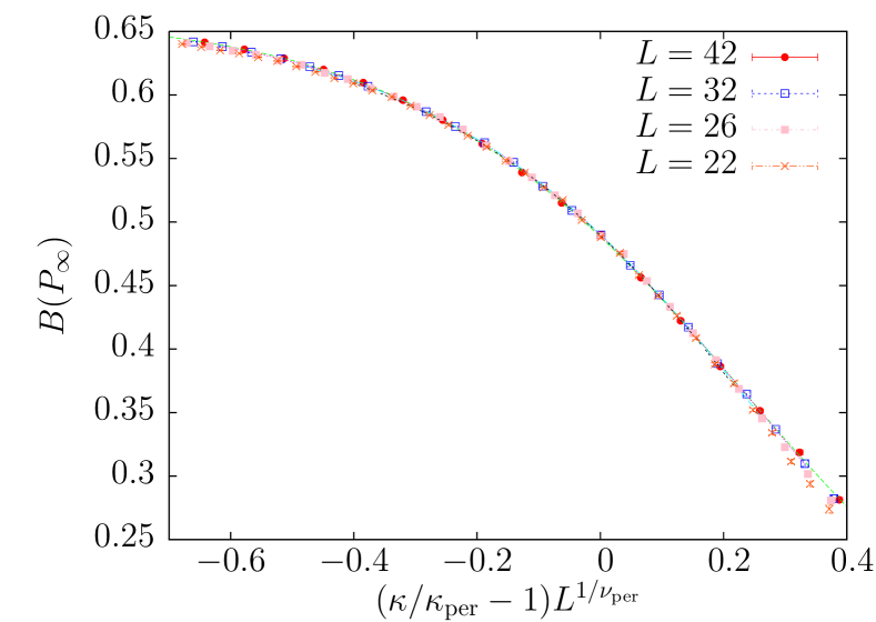
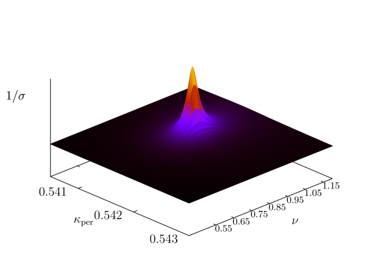
Figure 10: Top Left: Binder parameter of the percolation strength $P_{\infty}$ as a function of the hopping parameter $\kappa$. Top Right: Collapse of the data for $\kappa_{\mathrm{per}}=0.54145$ and $\nu_{\mathrm{per}}=0.881$. The data is obtained on lattices of linear size $L=22,26,30,42$. Bottom Left: Landscape of the quality of the data collapse over a range of values of $\kappa_{\mathrm{per}}$ and $\nu_{\mathrm{per}}$. The peak corresponds to the best collapse and yields our estimates $\kappa_{\mathrm{per}}=0.54145(2)$ and $\nu_{\mathrm{per}}=0.881(2)$.

To improve these estimates, we now apply our collapsing routine, rather than carrying out additional simulations for other lattice sizes. The method has the advantage that much more data is used as input for not only the locations of the peak maxima but all the data in the vicinity as well as the interpolated values obtained from reweighting are included. We take the Binder parameter $B(P_{\infty})$ of the percolation strength together with the scaling Ansatz

$$B(P_{\infty})=h\left(tL^{1/\nu_{\mathrm{per}}}\right),\quad t\equiv(\kappa-\kappa_{\mathrm{per}})/\kappa_{\mathrm{per}},$$ (15)

where $h$ is a scaling function. Figure 10 shows the raw data together with the data collapse for $\kappa_{\mathrm{per}}=0.54145$ and $\nu_{\mathrm{per}}=0.881$. The good quality of the data collapse is apparent from the 3D plot in the same figure. Given these estimates for $\kappa_{\mathrm{per}}$ and $\nu_{\mathrm{per}}$, we next apply the collapsing routine to determine the exponents $\beta_{\mathrm{per}}$ and $\gamma_{\mathrm{per}}$ from the scaling relations

$$P_{\infty}=L^{-\beta_{\mathrm{per}}/\nu_{\mathrm{per}}}f\left(tL^{1/\nu_{\mathrm{per}}}\right),\quad\chi(P_{\infty})=L^{\gamma_{\mathrm{per}}/\nu_{\mathrm{per}}}g\left(tL^{1/\nu_{\mathrm{per}}}\right)$$ (16)

with $f$ and $g$ scaling functions. Table 3 summarizes our results and compares them with the random percolation exponents.

Table 3: Critical exponents of the percolating vortex network across the Kertész line for $\beta=1.1$ and $\lambda=0.2$ compared with the standard percolation exponents.

Model	$\kappa_{\mathrm{per}}$	$\nu_{\mathrm{per}}$	$\beta_{\mathrm{per}}$	$\gamma_{\mathrm{per}}$
cAHM	0.54145(2)	0.881(2)	0.43(2)	1.76(2)
Percolation [46] (see also [47, 48])	-	0.8765(16)	0.4522(8)	1.7933(85)

In agreement with our conjecture [9], the estimates, which as shown in Fig. 11 lead to a good data collapse, are consistent with standard percolation exponents. Notice that, in contrast to the findings in the $|\phi|^{4}$ theory, the vortices appear to proliferate in the confinement phase after passing through the crossover region ($\kappa_{\mathrm{per}}<\kappa_{\times}$). We expect this to be related to the presence of monopoles which can act as sources for the vortices. To assess this, we study in the next section how the relative positions of the percolation threshold and the crossover region vary with changes in the parameters $\lambda$ and $\beta$.

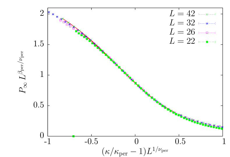
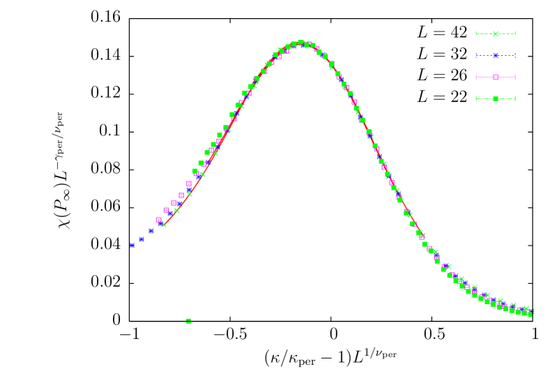
Figure 11: Left: Collapse of the percolation strength $P_{\infty}$ yielding an exponent $\beta_{\mathrm{per}}=0.43(2)$. Right: The same for the susceptibility $\chi(P_{\infty})$ yielding $\gamma_{\mathrm{per}}=1.76(2)$.

6 Fine Tuning

Since the vertex percolation threshold $\kappa_{\mathrm{per}}$ and the phase boundary $\kappa_{\mathrm{c}}$ coincide in the first-order transition region, it is expected that as we approach this region, the discrepancy found in the previous section at $\beta=1.1$ and $\lambda=0.2$ becomes smaller. To verify this, we repeat our analysis at $\beta=1.1$ and $\lambda=0.075$, which is closer to the first-order transition region. We find that the difference between the locations of the percolation threshold and the crossover determined using the overall vortex line susceptibility $\chi(v)$ indeed becomes smaller, changing from about $0.018$ at $\lambda=0.2$ to $0.007$ here. Moving in the opposite direction of increasing $\lambda$, we observe the discrepancy to increase, becoming as large as about $0.1$ in the London limit $\lambda\to\infty$. The percolation threshold still appears in the confinement phase after passing through the crossover region. That is, changes in the Higgs self-coupling $\lambda$ seem to leave the relative positions of the crossover and the apparent vortex proliferation threshold unchanged.

We next vary $\beta$ and set $\beta=2.0$ and $\lambda=0.2$. By increasing $\beta$, one suppresses the monopoles. They completely disappear in the limit $\beta\to\infty$, where the theory looses its compactness. Unfortunately, simulations at $\beta=2.0,\lambda=0.2$ are computationally much more challenging than at $\beta=1.1,\lambda=0.2$ as autocorrelation times are much longer. We therefore restrict ourselves to lattice sizes up to $L=36$. Moreover, observables other than percolation observables become less useful as can be seen from our example in Fig. 3. Whereas the susceptibility of the percolation probability has a pronounced peak and a clear maximum, the maximum in the coslink susceptibility $\chi(C)$ would be difficult to identify without reweighting. The large error bars obtained for the peak location of $\chi(C)$ reflect the absence of a pronounced peak.

Our main conclusion of the simulations at $\beta=2.0$ and $\lambda=0.2$ is that the locations of the apparent percolation threshold and the crossover determined using the overall vortex line susceptibility $\chi(v)$ have changed relative positions. This conclusion is based on Fig. 12 in which $\kappa_{\mathrm{per}}(L)$, estimated using different percolation observables, is plotted as a function of $1/L$ to see their tendency for $L\to\infty$. The first observation is that the data points are much closer to each other than was the case at $\beta=1.1$ (see Fig. 9). As before, $\kappa_{\mathrm{per}}(L)$ obtained from the susceptibility of the percolation strength (lowest set of data points) shows the largest corrections but increases monotonically for $L\to\infty$. The values $\kappa_{\mathrm{per}}(L)$ obtained from the percolation probability $P_{\mathrm{1D}}$ show less drastic corrections but are more difficult to extrapolate to the infinite-volume limit.

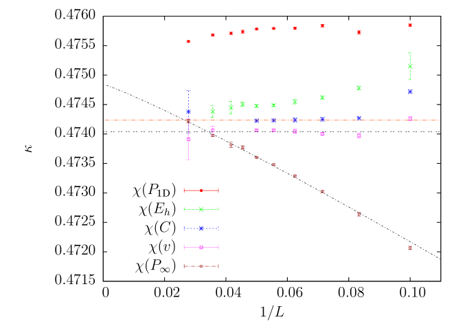
Figure 12: Locations of the susceptibility maxima of various observables as a function of $1/L$ for $\beta=2.0$.

The two sets of data points both extrapolate to a value around $\kappa_{\mathrm{per}}\approx 0.4748$ which follows from fitting $\chi(P_{\infty})$ to Eq. (14).

Figure 12 displays in addition to the locations of the susceptibility maxima of the vortex line density, also those of the coslink energy and the hopping energy. For $L>16$ the heights and locations of these susceptibilities remain constant, so that, as far as these observables are concerned, the infinite-volume limit is reached. The location of the crossover in the infinite-volume limit determined using these observables is below all estimates of the percolation threshold. In other words, while for $\beta=1.1,\lambda=0.2$, $\kappa_{\mathrm{per}}<\kappa_{\times}$, here the relative positions have changed, $\kappa_{\mathrm{per}}>\kappa_{\times}$, and the vortices proliferate already in the Higgs phase before entering the crossover region. By continuity we then expect at some value of $\beta$ in the interval $1.1<\beta<2.0$ the percolation threshold of the vortices to coincide with the location of the crossover. Since varying $\beta$ physically changes the monopole density, it is tempting to conclude that monopoles impede the formation of percolating vortex lines, and that by adjusting the monopole density, the location of the apparent vortex percolation threshold can be fine-tuned to coincide with that of the crossover. The use of the word “apparent” here is to underscore that vortex networks identified with our tracing rules are only an approximation to the true networks. The element of impediment introduced by the monopoles possibly plays a similar role as the stochastic element in the Fortuin-Kasteleyn construction of spin clusters in the Potts model [30].

We finally estimate the critical exponent $\nu_{\mathrm{per}}$ for $\beta=2.0$. Using the percolation probability as input observable for our collapsing routine, we arrive at the value $\nu_{\mathrm{per}}=0.88(1)$ and $\kappa_{\mathrm{per}}=0.4748(1)$. As a crosscheck we fit the scaling of $\chi(P_{\infty})$ with the lattice size $L$ to Eq. (14) giving $\nu_{\mathrm{per}}=0.88(8)$ and $\kappa_{\mathrm{per}}=0.47484(15)$ with a $\chi^{2}/\mathrm{DOF}=2.1$. This is again consistent with the standard percolation exponent. Although the relative positions of the apparent percolation threshold and the crossover have changed, variations in the inverse gauge coupling parameter $\beta$ appear not to change the value of this critical exponent.

7 Conclusions

The vortices arising in the compact Abelian Higgs model have been investigated by means of Monte Carlo simulations on a cubic lattice, and analyzed with the help of observables known from percolation theory. Because their behavior is more pronounced, percolation observables are better suited than other observables to probe the phase boundary, both in the first-order transition region as well as in the crossover region of the phase diagram. In the region where the Higgs and confinement phases are separated by a first-order transition, the vortices percolate right at the phase boundary. Since the rules applied to trace out the vortices result in networks that are in general only an approximation to the true ones, it is concluded that the discontinous first-order transition is forgivable of the resulting inaccuracies. The vortex network reflects the first-order nature of the transition in this region of the phase diagram. In the crossover region, the vortices still percolate. The percolation observables show second-order critical behavior along the Kertész line that is characterized by the usual percolation exponents. The location of the vortex percolation threshold estimated using percolation observables does not coincide with that of the crossover estimated using the vortex line density. Ideally, one would expect both to coincide. Also the $|\phi|^{4}$ theory in 3D, which undergoes a continuous phase transition, shows a similar behavior [29]. Whereas the estimate based on the line density coincides with the critical temperature, the estimates based on any of the percolation observables considered do not agree within error bars. This discrepancy may arise because the vortex networks are not correctly traced out or because a stochastic or impeding element in the construction of a network is missing. The monopoles appear to play such a role.

8 Acknowledgements

We wish to thank Arwed Schiller for useful discussions at an early stage of this project. S.W. acknowledges a PhD fellowship from the Studienstiftung desdeutschen Volkes. A.S. is indebted to Professor H. Kleinert for the kind hospitality at the Freie Universität Berlin. This work was partially supported by the Deutsche Forschungsgemeinschaft under grant Nos. JA483/22-1 and 23-1, a computer time grant on the JUMP computer of NIC at Forschungszentrum Jülich under project number HLZ12, and the EC Marie Curie Research and Training Network ENRAGE “Random Geometry and Random Matrices: From Quantum Gravity to Econophysics”, under grant No. MRTN-CT-2004-005616.

References

- [1] E. Fradkin and S. H. Shenker, Phys. Rev. D 19 (1979) 3682.
- [2] T. Banks and E. Rabinovici, Nucl. Phys. B 160 (1979) 349.
- [3] K. C. Bowler, G. S. Pawley, B. J. Pendleton, D. J. Wallace, and G. W. Thomas, Phys. Lett. B 104 (1981) 481.
- [4] A. M. Polyakov, Nucl. Phys. B 120 (1977) 429.
- [5] Y. Munehisa, Phys. Lett. B 155 (1985) 159.
- [6] G. N. Obodi, Phys. Lett. B 174 (1986) 208.
- [7] A. Kovner and B. Rosenstein, Int. J. Mod. Phys. A 7 (1992) 7419.
- [8] G. Bhanot and B. A. Freedman, Nucl. Phys. B 190 (1981) 357.
- [9] S. Wenzel, E. Bittner, W. Janke, A. M. J. Schakel, and A. Schiller, Phys. Rev. Lett. 95 (2005) 051601.
- [10] S. Mandelstam, Phys. Rept. 23 (1976) 245.
- [11] G. ’t Hooft, Nucl. Phys. B 138 (1978) 1.
- [12] M. B. Einhorn and R. Savit, Phys. Rev. D 19 (1979) 1198.
- [13] J. Kertész, Physica A 161 (1989) 58.
- [14] K. Langfeld, in Strong and Electroweak Matter 2002, Proceedings of the Workshop On Strong And Electroweak Matter, Heidelberg, Germany, 2 – 5 October 2002, edited by M. G. Schmidt (World Scientific, Singapore, 2003).
- [15] R. Bertle, M. Faber, J. Greensite, and S. Olejnik, Phys. Rev. D 69 (2004) 014007.
- [16] H. Satz, Nucl. Phys. A 681 (2001) 3.
- [17] M. N. Chernodub, F. V. Gubarev, E.-M. Ilgenfritz, and A. Schiller, Phys. Lett. B 434 (1998) 83.
- [18] M. N. Chernodub, F. V. Gubarev, E.-M. Ilgenfritz, and A. Schiller, Phys. Lett. B 443 (1998) 244.
- [19] R. Bertle and M. Faber, in Quark Confinement and the Hadron Spectrum V, Proceedings of the 5th International Conference, Gargnano, Italy, 10 – 14 September 2002, edited by N. Brambilla and G. M. Prosperi (World Scientific, Singapore, 2002).
- [20] K. Langfeld, O. Tennert, M. Engelhardt, and H. Reinhardt, Phys. Lett. B 452 (1999) 301.
- [21] M. Engelhardt, K. Langfeld, H. Reinhardt, and O. Tennert, Phys. Rev. D 61 (2000) 054504.
- [22] K. Langfeld, Phys. Rev. D 67 (2003) 111501.
- [23] S. Wenzel, E. Bittner, W. Janke, A. M. J. Schakel, and A. Schiller, POS LAT2005 (2005) 248.
- [24] D. Stauffer and A. Aharony, Introduction to Percolation Theory, 2nd ed. (Taylor and Francis, London, 1994).
- [25] M. N. Chernodub, E.-M. Ilgenfritz, and A. Schiller, Phys. Lett. B 547 (2002) 269.
- [26] M. N. Chernodub, R. Feldmann, E.-M. Ilgenfritz, and A. Schiller, Phys. Rev. D 70 (2004) 074501.
- [27] S. Takashima, I. Ichinose, T. Matsui, and K. Sakakibara, Phys. Rev. B 74 (2006) 075111.
- [28] K. Kajantie, M. Laine, T. Neuhaus, A. Rajantie, and K. Rummukainen, Phys. Lett. B 482 (2000) 114.
- [29] E. Bittner, A. Krinner, and W. Janke, Phys. Rev. B 72 (2005) 094511.
- [30] C. M. Fortuin and P. W. Kasteleyn, Physica 57 (1972) 536.
- [31] M. N. Chernodub, R. Feldmann, E.-M. Ilgenfritz, and A. Schiller, Phys. Lett. B 605 (2005) 161.
- [32] W. Janke and A. M. J. Schakel, in Order, Disorder and Criticality, Advanced Problems of Phase Transition Theory, Vol. 2, edited by Y. Holovatch (World Scientific, Singapore, 2007), p. 123.
- [33] B. A. Berg and T. Neuhaus, Phys. Rev. Lett. 68 (1992) 9.
- [34] W. Janke, in Computer Simulations of Surfaces and Interfaces, edited by B. Dünweg, D. P. Landau, and A. I. Milchev (Kluwer, Dordrecht, 2003), p. 137.
- [35] K. Kajantie, M. Laine, K. Rummukainen, and M. Shaposhnikov, Nucl. Phys. B 466 (1996) 189.
- [36] B. Bunk, Nucl. Phys. B (Proc. Suppl.) 42 (1995) 566.
- [37] A. M. Ferrenberg and R. H. Swendsen, Phys. Rev. Lett. 61 (1988) 2635.
- [38] A. M. Ferrenberg and R. H. Swendsen, Phys. Rev. Lett. 63 (1989) 1195.
- [39] W. H. Press, B. P. Flannery, S. A. Teukolsky, and W. T. Vetterling, Numerical Recipes: The Art of Scientific Computing, 2nd ed. (Cambridge University Press, Cambridge and New York, 1992).
- [40] R. P. Brent, Algorithms for Minimization without Derivatives (Prentice-Hall, Englewood Cliffs, NJ, 1973).
- [41] B. Efron, The Jackknife, the bootstrap, and other resampling plans (Society for Industrial and Applied Mathematics [SIAM], Philadelphia, 1982).
- [42] L. Wang, K. D. S. Beach, and A. W. Sandvik, Phys. Rev. B 73 (2006) 014431.
- [43] M. Galassi et al., GNU Scientific Library Reference Manual, 2nd ed. (Network Theory Limited, 2003).
- [44] S. M. Bhattacharjee and F. Seno, J. Phys. A 34 (2001) 6375.
- [45] W. Janke, Phys. Rev. B 47 (1993) 14757.
- [46] H. G. Ballesteros, L. A. Fernandez, V. Martin-Mayor, G. Parisi, and J. J. Ruiz-Lorenzo, J. Phys. A 32 (1999) 1.
- [47] Y. Deng and H. W. Blöte, Phys. Rev. E 72 (2005) 016126.
- [48] M. Hellmund and W. Janke, Phys. Rev. E 74 (2006) 051113.