Reliability of temporal coding on pulse-coupled networks of oscillators
Abstract
We study the reliability of spike output in a general class of pulse-coupled oscillators receiving a fluctuating input. Showing that this problem is equivalent to noise-induced synchronization between identical networks of oscillators, we employ the phase reduction method to analytically derive the average Lyapunov exponent of the synchronized state. We show that a transition occurs between reliable and unreliable responses at a critical coupling strength, which is determined through the competition between the external input and recurrent input. To our surprise, the critical value does not depend on intrinsic properties of oscillators.
pacs:
05.45.Xt, 02.50.Ey, 05.10.Gg, 87.18.SnNoise-induced synchronization appears in a variety of phenomena including lasers laser , chemical reactions chemical , gene networks gene and neuronal systems mainen ; neuron . In these systems, periodic or chaotic oscillators driven by a common fluctuating input synchronize with each other due to the nonlinearity of oscillators and the stochastic nature of the input nis . The phase reduction kuramoto and the Lyapunov analysis proved that two or more identical oscillators receiving a common fluctuating input are always in-phase synchronized regardless of their intrinsic properties and initial phases teramae ; piko_nakao . We can interpret such oscillators as a single oscillator receiving the same input repeatedly, but with different initial phases, i.e. many trials of an input application. Therefore, the in-phase synchronization of input-driven oscillators implies, in a single oscillator, the reproducibility of the responses to a repeated input, or response reliability, which is particularly important for processing external signals. Reliable responses to a fluctuating input are actually measured from single cortical neurons mainen . However, neurons and other oscillators in the real world work collectively in their networks rather than individually. To study whether a network of oscillators still has response reliability, we develop a theory of noise-induced synchronization between networks of oscillators rather than between single oscillators. We find a transition from reliable to unreliable responses at a critical coupling strength. Deriving average Lyapunov exponent analytically, we reveal that the critical value is determined through the competition between variance of the external input and of internal recurrent inputs regardless of details of oscillators. Around the transition point where magnitude of the average Lyapunov exponent is small, information of initial states can stay in the network for a long time. We discuss a possible role of the long time scale in role-sharing between rate and temporal coding on neuronal computation in the brain.
A network of pulse-coupled limit-cycle oscillators receiving fluctuating inputs are described as:
| (1) |
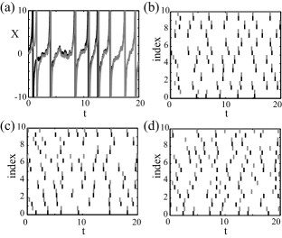
where and has a stable limit-cycle solution . A unit vector indicates the direction of interactions in the multidimensional space spanned by . We assume, with neuronal oscillators in mind, coupling matrix is a sparse random matrix with connection probability , and each nonzero component of is either or if refers to an excitatory or an inhibitory cell, respectively. The network consists of excitatory neurons and inhibitory neurons. Fluctuating external inputs represent independent white Gaussian processes with strength , and represents spike times of the th neuron. We use as a control parameter of the network and require, for simplicity, that is in proportional to and satisfies the balance condition balance ; vreeswijk , , whereas results of the paper are independent of the restriction. When , response of oscillators are always reliable, i.e. the spike sequence of each oscillator converges into the same sequence in different trials. Figure 1a and 1b demonstrates the reliable responses obtained from numerical calculations of quadratic integrate-and-fire (QIF) neurons, , with variable resetting qif . Whereas two trials start from different initial states, raster plots of them converge into same sequences, i.e. same spike times. We then introduce finite couplings to the network of oscillators and calculate firing responses in a similar way to Fig. 1b. When coupling strength is small, the population is still reliable, spike sequences of different trials converge into the same one (Fig. 1c). However, the reliability is lost from the population when coupling strength is sufficiently large (Fig. 1d). Spike sequences of two trials never converge into the same one while we apply the same input to trials. In terms of synchronization, the result means that fluctuating inputs induce phase synchronization to two identical networks of oscillators only when coupling strength of the network is sufficiently weak.

Regarding the fluctuating signals and recurrent connections as perturbations to the deterministic oscillators, we apply the standard phase reduction method to Eq. (1) and obtain stochastic equations of phases as,
| (2) |
where is an intrinsic frequency of the unperturbed oscillators. Phase sensitivity function or phase response function is defined uniquely from as kuramoto . To simplify notations, we assumed without loss of generality that is in parallel with and replaced vector variables and to scalar variables and in Eq. (2). For the QIF model, for instance, , . Note that discontinuous variable resetting is now reduced to continuous dynamics over a spike threshold because derivation of is continuous between and , . To avoid unrealistic cases where an oscillator sends numerous spikes within a short interval of time when its fluctuating phase crosses the firing threshold, should be vanish around the threshold. Realistic neuron models including the QIF model satisfy the condition. Reliability of the firing responses is equivalent to that of phase dynamics because phase deviation is proportional to deviation of firing time. Phases of two trials, and evolve satisfying Eq. (2) from different initial phases but receiving same inputs, , in the same network, . Since phase synchronized state, , is an obvious solution of these two equations, linear stability around the solution determines the response reliability. To evaluate the stability we linearize Eq. (2) in terms of small phase differences, , and calculate average Lyapunov exponent arnold over all oscillators in the network.
Coupling terms are linearized as follows. Consider increment of , when th cell fires. We can take firing time of is , firing time of is therefore . We can assume without loss of generality. At , receives a spike from ,
| (3) |
Phases evolve as follows from to , because is a short interval,
| (4) |
where . In order to evaluate phase responses at precise timings just before spike inputs, we translated Eq. (2) to equivalent Ito integrals in Eq. (4) strato . Third terms of Eq. (4) result from the translation. Finally, at , receives a spike from ,
| (5) |
We can linearize from Eq. (3) to (5) in terms of with an attention that is the order of and then the order of . Taking all connections into account and neglecting terms higher than the order of , we obtain linearized equation of as
By introducing new variables , Eq. (Reliability of temporal coding on pulse-coupled networks of oscillators) is further rewritten as
Since the Lyapunov exponent is defined as , the long time average of the Eq. (Reliability of temporal coding on pulse-coupled networks of oscillators) coincides with . We assume that the network is in asynchronous steady firing state due to fluctuating inputs and replace spike times of cells by independent Poisson processes with firing rate asynchro . Then averaging of Eq. (Reliability of temporal coding on pulse-coupled networks of oscillators) over the Poisson processes and over all oscillators in the network gives
| (8) |
where . Here we used the assumption of weak inputs and weak interactions and reduced distributions of phases to uniform distributions in . Unfortunately, Eq. (8) is not a closed form of . However, when variance of is small, or , the last term of Eq. (8) is approximated as and we finally obtain the following main formula of the average Lyapunov exponent:
| (9) |
Note that when variance of is not small, Eq. (9) gives the lower bound of because in generally.
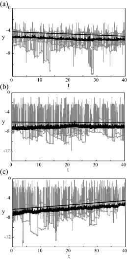
To confirm the above analysis, we calculate averaged dynamics of numerically for networks of QIF oscillators. Due to fluctuating inputs and recurrent interactions, themselves do not evolve monotonically. However, population averages of decrease or increase almost linearly depending on coupling strengths g as predicted by Eq. (9).

Our expression of the Lyapunov exponent, Eq. (9), tells us two important facts of the reliability transition. First, the transition stems from a competition between two variances, variance of input signals and variance of recurrent inputs . Whereas the first contribution to the exponent is negative, the second is always positive. Therefore, the network lost their reliability when the second exceeds the first. Second, the factor of which reflects intrinsic properties of oscillators is multiplied equivalently to these two factors and in Eq. (9). Therefore, the critical coupling strength , given as the solution of , is universal in the sense that is independent of details of oscillators. For the network structure we used in Fig. 1, the critical value is given as regardless of oscillators on the network. If we use another natural normalization of coupling strengths as vreeswijk , we can eliminate from the critical strength, .
In the vicinity of the critical coupling strength where , information on the initial states of oscillators may disappear quite slowly after the onset of input. This slow transient behavior might have the following implications for computations by cortical networks. The output of the computation is not simply determined by the current input, but is also modulated by the brain’s internal state and/or input histories history ; liquid . In our model, the membrane time constant sets the short time scale that enables the network to respond quickly to an external input with firing rate of population dynamics vreeswijk ; rate . By contrast, the critical dynamics of temporal spike sequences may set a much longer time scale to ensure the response diversity reflecting the initial state or input histories. This implies that neuronal populations may simultaneously achieve two different time scales by parallel use of rate code and temporal code. Further studies are required for clarifying this possibility.
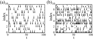
So far, we have restricted our study to super-threshold neurons which continue to fire without external inputs. Numerical simulations of sub-threshold QIF model with , however, suggest that similar transition also occurs in a network of sub-threshold neuron models (figure 3). It remains unknown whether this transition may appear in a broad class of sub-threshold neuron models because the phase reduction method is not applicable to sub-threshold neuron models. A unified treatment of super- and sub- threshold neuron models is awaited. We have assumed that couplings among oscillators are delta-functions. To remove a doubt that our results might be pathological phenomena come from singularity of delta-functions, we calculated reliability of coupled oscillators numerically using a alpha-function, , instead of . Again, we could see similar transition from reliable to unreliable responses (results not shown). Linear integrate-and-fire model is the most useful description of firing neurons. This model, however, behave unrealistically about response reliability even when because of its anomalous variable resetting teramae ; lif . Here, we use quadratic integrate-and-fire model to avoid the problem. Coupled oscillators may synchronize with each other if is sufficiently large, whereas we have only concentrated on the asynchronous steady state. Synchronization may affect average Lyapunov exponent and may change the transition significantly because we must use correlated stochastic processes instead of independent Poisson processes when we average Eq. (8) to obtain .

In conclusion, coupled reliable elements are not necessarily reliable any more. Spike responses of coupled oscillators to fluctuating inputs show transition from reliable responses to unreliable responses. In terms of noise-induced synchronization, common noises fail to induce phase synchronization to networks of strongly coupled oscillators whereas same inputs always induce synchronization to single oscillators. Underlying mechanism of the transition is competition between a variance of external signals and a variance of internal recurrent inputs. Critical coupling strength derived analytically is independent of details of oscillators because phase response functions appear equivalently in these competing factors.
We thank Y. Tsubo and H. Cateau for fruitful discussions and valuable comments. The present work was supported by Grant-in-Aid for Young Scientists (B) 50384722 and Grant-in-Aid for Scientific Research 17022036 from the Japanese Ministry of Education, Culture, Sports, Science and Technology.
References
- (1) A. Uchida, R. McAllister, and R. Roy, Phys. Rev. Lett. 93, 244102 (2004).
- (2) I. Z. Kiss, J. L. Hudson, J. Escalona, and P. Parmananda, Phys. Rev. E 70, 026210 (2004).
- (3) T. Zhou, L. Chen, and K. Aihara, Phys. Rev. Lett. 95, 178103 (2005).
- (4) Z. F. Mainen and T. J. Sejnowski, Science 268, 1503 (1995).
- (5) R. V. Jensen, Phys. Rev. E 58, R6907, (1998); J. Ritt, Phys. Rev. E 68, 041915, (2003); E. K. Kosmidis and K. Pakdaman, J. Comput. Neurosci. 14, 5, (2003); R F. Galán, N. Fourcaud-Trocmé, G. B. Ermentrout, and N. N. Urban, J. Neurosci. 26, 3646 (2006).
- (6) A. S. Pikovsky, In R. Z. Sagdeev, Editor, Nonlinear and Turbulent Processes in Physics, 1601, Harwood, Singapore (1984); C. Zhou, J. Kurths, Phys. Rev. Lett. 88, 230602 (2002).
- (7) Y. Kuramoto, Chemical Oscillation, Waves, and Turbulence (Springer-Verlag, Tokyo, 1984); (Dover Edition, 2003).
- (8) J. N. Teramae and D. Tanaka, Phys. Rev. Lett. 93, 204103 (2004); Prog. Theor. Phys. Suppl. 161, 360 (2006).
- (9) D. S. Goldobin and A. Pikovsky, Phys. Rev. E 71, 045201(R) (2005); Phys. Rev. E 73, 061906 (2006); K. Nagai, H. Nakao, and Y. Tsubo, Phys. Rev. E 71, 036217 (2005); H. Nakao et al., Phys. Rev. E 72, 026220 (2005); H. Nakao, K. Arai, and Y. Kawamura, Phys. Rev. Lett. 98, 184101 (2007).
- (10) M. N. Shadlen andW. T. Newsome, Curr. Opin. Neurobiol. 4, 569 (1994); Y. Shu, A. Hasenstaub, and D. A. McCormick, Nature 423 288 (2003).
- (11) C. van Vreeswijk, and H. Sompolinsky, Science 274, 1724 (1996); C. van Vreeswijk, and H. Sompolinsky, Neural Comput. 10, 1321 (1998).
- (12) G. B. Ermentrout, and N. Kopell, SIAM J. Appl. Math. 46, 233 (1986); N. Brunel, and P. E. Latham, Neural Comput. 15, 2281 (2003).
- (13) L. Arnold, Random Dynamical Systems (Springer-Verlag, Berlin, 1998).
- (14) R. L. Stratonovich, Topics in the Theory of Random Noise (Gordon and Breach, New York, 1963).
- (15) L. F. Abbott and C. van Vreeswijk, Phys. Rev. E 48, 1483 (1993). N. Brunel, J. Comput. Neurosci. 8, 183 (2000);
- (16) A. Arieli, A. Sterkin, A. Grinvald, Ad Aertsen Science 273, 1868 (1996); M. Tsodyks, T. Kenet, A. Grinvald, and A. Arieli, Science 286, 19433 (1999)
- (17) W. Maass, T. Natschläger, and H. Markram, Neural Comput. 14, 2531 (2002); H. Jaeger and H. Haas Science 304, 78 (2004).
- (18) M. V. Tsodyks and T. Sejnowski, Netwok 6, 111 (1995); N. Fourcaud, N. Brunel, Neural Comput. 14, 2057 (2002).
- (19) S. Coombes, Phys. Lett. A 255, 49 (1999); T. Tateno, Phys. Rev. E, 65, 021901 (2002).