Multiple complex networks emerging from individual interactions

Abstract

Systems composed of distinct complex networks are present in many real-world environments, from society to ecological systems. In the present paper, we propose a network model obtained as a consequence of interactions between two species (e.g. predator and prey). Fields are produced and sensed by the individuals, defining spatio-temporal patterns which are strongly affected by the attraction intensity between individuals from the same species. The dynamical evolution of the system, including the change of individuals between different clusters, is investigated by building two complex networks having the individuals as nodes. In the first network, the edge weight is given by the Euclidean distance between every two individuals and, in the case of the second network, by the amount of time two individuals stay close one another. A third network is obtained from the two previous networks whose nodes correspond to the spatially congruent groups. The system evolves to an organized state where Gaussian and scale-free-like strength distributions emerge, respectively, in the predator and prey networks. Such a different connectivity is mainly a consequence of preys elimination. Some configurations favor the survival of preys or higher efficiency of predator activity.

I Introduction

Despite the impressive development undergone by complex networks along the recent years, relatively little attention has been focused on the investigation of systems incorporating more than one network, and even lesser attention has been given to the study of specific dynamics (at the nodes or of the own network topology) taking place in such networks. Yet, several real-world systems are inherently composed by multiple networks. In biological sciences, for instance, protein-protein interaction networks are immediately related to transcriptional and metabolic networks OltvaiPyramid02 . Similar entanglements are found in many other areas, such as in the Internet or in the www, which are directly related to social and cultural networks, as well as economical constraints CostaMultiple05 . Strictly speaking, it is actually hard to think of a real-world system which can be completely represented in terms of a single network.

Some works considering multiple networks have been reported in the literature. The “Solomon Network” system was introduced by Erez and collaborators Erez05 . It consists in a multi-layered system with a set of nodes (agents) common to all layers. In each layer, different rules according to social and/or economical ties define the interaction between the nodes. On the other hand, the coupling between layers is obtained by interaction between variables associated to the respective nodes in different layers. Another layered-based formalism was proposed independently by Kurant et al. Kurant06a . Using transportation networks, they constructed a logical network representing the traffic flows which were mapped onto another network representing the physical infrastructure Kurant06a ; Kurant06b . Park et al. constructed two networks of musicians in which the edges of one network represented the similarity while, in the other, they represented the collaboration between the musicians Park06 . The intersection of both networks generated a new dataset where the structural properties showed significant differences between both types of networks. We have been particularly interested in addressing the dynamics of multiple networks systems. In a previous work Rocha07 , we considered a system composed of regular and complex networks. While a diffusion pattern evolved in the regular network, the complex network were expected to self-organize to control and if possible, eliminate the pattern. An interaction rule between both networks was responsible to activate the complex network nodes.

Of special relevance in which concerns multi-layered system are ecological environments where the evolution is constrained by the interactions among its components, besides climate conditions and other external influences. Modelling all such constrains might be difficult and often unnecessary while investigating specific phenomena of interest. Considering an ideal environment (favorable climate and abundant supplies), the interaction between animals could be described as an interaction function representing the odor intensity Mingfeng:odor . Conversely, the interaction rule could be avoided to some extent as in the famous Lotka-Volterra system (predator-prey model) Lotka_book ; Volterra_book , which considers only the amount of individuals of one species as a constrain to the evolution of the other species. Adding a diffusive term generalizes the system in which concerns spatial constraints, but does not properly address the question of single interactions Murray_book . Although collective behavior may emerge from such simple interaction rules Waldau:book ; Sznajd:opinion ; Farkas:mexicanwave , there are open questions related to emergence of spatio-temporal patterns on complex adaptive systems. Since the predator prey dynamics involves two types of agents (or individuals) in constant interaction, we considered a multi networks view of the system evolution. In this case, each network with moveable nodes represents one species, while the interaction rule between the nodes of both networks is defined in terms of sensitive fields.

More specifically, in the present paper we propose a system composed of two interacting species, with emphasis on the representation of the spatial position of each individual. One of the species (henceforth called predator) relies on the other species (prey) as the only source of food. In this scarce food environment, predators move by sensing the presence of preys while the preys are expected to sense the predators proximity and move away. Mutual attraction between same species individuals tends to generate spatial clusters which imply decrease in the mobility of single individuals inside those clusters. Two weighted complex networks are constructed along all time steps in terms of the dynamics between predators and preys. One of them expresses the Euclidean distance between any two animals as weights. This network is geographical, in the sense that the each node incorporate information about the position of the respective individual. In the other network, the weights reflect the history of proximity between pairs of animals. In other words, the weights in the second network are proportional to the total time each pair of animals spend together. A third network is obtained so that each of its nodes corresponds to one spatial cluster and the weights provide information about the number of exchanges of animals between pairs of respective spatial clusters.

The current paper begins by reviewing basic concepts related to complex networks and follows stating the interaction rules of the proposed model and the parameters of the system. The results section discusses the emergence of spatial clusters patterns and then analyse the evolution of structural properties of the resulting complex network and their relation with the proposed dynamics.

II Complex Networks Concepts

A complex network $\Gamma$ with $N$ nodes can be defined by a set $V(\Gamma)$ of nodes $\mu_{i}$ ($i=1,2,\ldots,N$) and a set of edges $E(\Gamma)$ connecting a pair of nodes $(\mu_{i},\mu_{j})$. Given a set $W(\Gamma)$ of real values, a weight $\omega_{\mu_{i},\mu_{j}}$ is assigned to an edge by mapping one element of $W(\Gamma)$ to one element of $E(\Gamma)$. A sub-network $\kappa$ is defined by a set of nodes $V(\kappa)\subset V(\Gamma)$ and a set of edges $E(\kappa)\subseteq\{(\mu_{i},\mu_{j}):(\mu_{i},\mu_{j})\in E(\Gamma)\text{ and }\mu_{i},\mu_{j}\in V(\kappa)\}$. The sub-network $\kappa$ is connected if and only if, any node of $V(\kappa)$ can be reached by any other node of $V(\kappa)$ Barabasi:review ; Newman:review ; Dorog:review ; Boccaletti:review ; Costa:review .

The local connectivity of a node $\mu_{i}$ can be quantified by its degree $k_{i}$, which provides the number of nodes directly connected to $\mu_{i}$, i.e. the neighbours of $\mu_{i}$. When the connections have weights, the strength $s_{i}$ of node $\mu_{i}$ is obtained by summing all weights assigned to connections involving $\mu_{i}$ Costa:review . The number of closed triangles in the neighbourhood of node $\mu_{i}$ is given by the generalized clustering coefficient $cc_{i}$ (eq. 1) which considers the weights $\omega_{\mu_{i},\mu_{j}}$ of each connection established between a node $\mu_{i}$ and its neighbours $\mu_{j}$ Barrat:weight .

$$cc_{i}=\dfrac{1}{s_{i}(k_{i}-1)}\sum_{j,k=1}^{N,N}\dfrac{\omega_{\mu_{i},\mu_{j}}+\omega_{\mu_{i},\mu_{k}}}{2}a_{ij}a_{ik}a_{jk}$$ (1)

where, $a_{ij}$ represents the connection between $\mu_{i}$ and $\mu_{j}$ such that $a_{ij}a_{ik}a_{jk}=1$ indicates that a closed triangle exists in the neighbourhood of node $\mu_{i}$. Finally, the overall structure of a network can be summarized by the averaged value of each considered measurement.

III Interaction Model

III.1 Movement and Interaction Dynamics

Consider a squared bi-dimensional region $O$ of size $L=512$ in the continuous space $\Omega$. We randomly distribute $N=300$ animals (or individuals $I_{i}$, where: $i=1,2,\ldots,N$) of each species (predator and prey) inside $O$ such that any two species-independent individuals $I_{i}$ and $I_{j}$ are at a minimum Euclidean distance $r_{i,j}=R_{min}=4$ from each other. At every time step $\Delta t=0.1$, each individual $I_{i}$ updates its respective position $P^{t}_{x_{i},y_{i}}$ according to $P^{t+1}_{x_{i},y_{i}}=P^{t}_{x_{i},y_{i}}+\mathbf{v_{i}}\Delta t$. The resulting sensitive field is understood to provide the velocity $\mathbf{v_{i}}$ of each individual at any position and time. In such a way, an animal only senses other individuals within its perception radius, which is fixed over time as $R_{per}=128$.

The interactions between predators and preys are directly related to their species. In case they belong to the same species, the sensitive field generated by one over the other is given by a dimensionless function (eq. 2a), where the parameters $\lambda=4.0$ and $\mu=0.04$ have respectively units of $[L]$ and $[L]^{-2}$. The alternate characteristic of the function $g(r_{i,j})$ is chosen because it provides a balance of attraction and repulsion between same species. On the other hand, when the animals belong to different species, the individual $I_{i}$ of one species senses $I_{j}$ of the other species in such a way that its reaction intensity is inversely proportional to the proximity between them. This is expressed in equation 2b, where the parameter $\sigma=1.0$ has units of area $[L]^{2}$.

$$\textbf{g}_{j}(r_{i,j}) =\Bigl{[}4e^{-\mu{(r_{i,j}-\lambda)}^{2}}-e^{-\mu{(r_{i,j}-3\lambda)}^{2}}\Bigr{]}\text{\^{r}}_{i,j}$$ (2a)

$$\textbf{f}_{j}(r_{i,j}) =\dfrac{\sigma}{r_{i,j}^{2}}\text{\^{r}}_{i,j}\qquad\text{ where: }\;\;\|\textbf{r}_{i,j}\|<R_{per}$$ (2b)

The sum over all contributions $I_{j}$ determines the direction and intensity of an individual $I_{i}$ final velocity (eq. 3). The signs and values of the parameters $\alpha$ and $\beta$ in equation 3 should be selected so as to correctly represent the system of interest, and they have units of velocity $[L][T]^{-2}$. In the present paper, we will investigate different combinations of the parameter $\beta$ for predators and preys (eq. 4).

$$\textbf{v}_{i}=\alpha\sum_{j=1}^{N-1}\textbf{f}_{j}(r_{i,j})+\beta\sum_{j=1}^{N-1}\textbf{g}_{j}(r_{i,j})$$ (3)

$$\left\{\begin{array}[]{llll}\text{Predator:}&\alpha_{predator}\;<0&\text{ and }&\beta_{predator}\;\geqslant 0\\ \text{Prey:}&\alpha_{prey}\;>0&\text{ and }&\beta_{prey}\;\geqslant 0\end{array}\right.$$ (4)

Since the model is motivated by an ecological environment, we suppose that preys have plenty of food. Consequently, a prey $I_{j}$ only dies when close enough $r_{i,j}\leqslant R_{eli}=4$ to a predator $I_{i}$. The conservation of the number of animals is provided by a feedback process where each eliminated prey is promptly replaced by a new one. The feedback process consists in randomly arranging the new preys within the region $O$, while respecting the minimum distance $R_{min}=4$ between two individuals as in the initial conditions. As the abundance of preys provides enough resources to predators, we suppose that they never die along the simulation interval.

Although periodic boundary conditions are usually adopted in order to minimize finite size effects, an ecological system is often better described by other types of boundary conditions. In fact, animals tend to live inside a specific region $O$ of the ecosystem $\Omega$ called habitat (Similarly, people use to restrict their everyday life within cities or even within home, work and school places). The habitat contains not only one species, but also many animal and vegetal species, which constitute a rich environment. Consequently, the animals are able to interact with a number of species enclosed in such a region. The boundaries of the habitat can be related to landmarks such as mountains and rivers, or even islands. In order to reproduce such real boundary constrains, we adopt elastic boundaries conditions (eq. 5) which restrict the movement region but also allow preys to escape while close to the edges.

$$\left\{\begin{array}[]{llll}\text{If }&x(y)>L&\text{then }&x(y)\leftarrow 2L-x(y)\\ \text{If }&x(y)<0&\text{then }&x(y)\leftarrow|x(y)|\\ \end{array}\right.$$ (5)

III.2 Complex Networks Construction

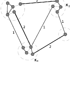
At each time step, a geographical and weighted network fully connected $\Gamma_{geo}$ is obtained by associating a node $\mu_{i}$ to each individual $I_{i}$ of both species and setting the weight $\omega_{\mu_{i},\mu_{j}}$ of each edge as the Euclidean distance $r_{i,j}$ between the respective two individuals. Since the animals are constantly moving throughout the sub-space $O$, the network $\Gamma_{geo}$ has a dynamical structure which changes at every step. By eliminating the edges above a threshold $T=30$ and setting $\omega_{\mu_{i},\mu_{j}}=1$ for the others, we obtain a new complex network $\Gamma^{\prime}_{geo}$ fragmented in many connected sub-networks $\kappa_{k}$ which we call spatial groups (Fig. 1-a).

The second complex network $\Gamma_{his}$ is constructed by considering the history of proximity between every two nodes of $\Gamma_{geo}$ (Fig. 1-a). The nodes $V(\Gamma_{his})\Leftrightarrow V(\Gamma_{geo})$ are initially fully connected so that each edge is set with $w_{\mu_{i},\mu_{j}}=0$. Whenever two individuals $I_{i}$ and $I_{j}$ fall close enough ($r_{i,j}\leqslant T=30$), the weight $w^{t+1}_{\mu_{i},\mu_{j}}=w^{t}_{\mu_{i},\mu_{j}}+1$ is updated. The connections involving dead preys are immediately eliminated.

(a)                                                      (b)

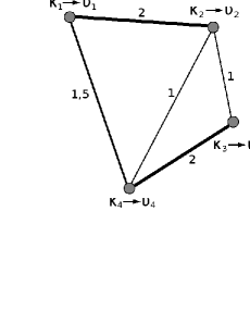
Figure 1: (a) A sample of both networks where the nodes represent the individuals. Light-gray edges belong to $\Gamma^{\prime}_{geo}$ and black edges to network $\Gamma_{his}$. Dashed lines emphasize the sub-networks $\kappa_{k}$. (b) The resulting network $\Gamma_{res}$ is obtained by merging $\Gamma^{\prime}_{geo}$ and $\Gamma_{his}$. Each node $\upsilon_{k}$ of $\Gamma_{res}$ is related to one sub-network $\kappa_{k}$ in Figure 1-a. In both Figures, the edge thickness is proportional to the respective weight.

The resulting network $\Gamma_{res}$ is obtained by a merging mechanism which is done by associating a node $\upsilon_{k}$ to each sub-network $\kappa_{k}$ of $\Gamma^{\prime}_{geo}$ such that a new set of nodes $V(\Gamma_{res})$ is obtained. If $M$ is the number of edges between the sub-network $\kappa_{k}$ and $\kappa_{l}$, the weight $\Xi_{k,l}$ (eq. 6) of the corresponding edge $(\upsilon_{k},\upsilon_{l})$ in $\Gamma_{res}$ is given by the average value of $w_{\mu_{i},\mu_{j}}$ established between the members $\mu_{i}$ and $\mu_{j}$ of different spatial groups $\kappa_{k}$ (Fig. 1-b).

$$\Xi_{\upsilon_{k},\upsilon_{l}}=\dfrac{1}{M}\sum_{\mu_{i},\mu_{j}}w_{\mu_{i},\mu_{j}}\quad\text{where: }\mu_{i}\subseteq V(\kappa_{k})\text{ and }\mu_{j}\subseteq V(\kappa_{l})$$ (6)

IV Cluster Emergence

IV.1 Spatio-temporal patterns

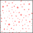
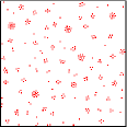
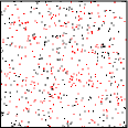
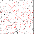
The interaction between different species, along with the prey replacement mechanism, are fundamental for providing a non-stationary state. Spatio-temporal cluster patterns emerge from the dynamics due to interaction between same specie individuals. In the absence of one species the system evolves to a stable state with many small static clusters (Fig. 2). Contrariwise, in the presence of interacting preys and predators, but null attraction between same specie individuals, the system evolves to a non-stable state, without emergence of clusters (Fig. 3).

(a) $t=250000$     (b) $t=500000$

Figure 2: Snapshots of the emergent spatio-temporal pattern for one single species with $\beta=0.125$.

(a) $t=250000$     (b) $t=500000$

Figure 3: Snapshots of predators (red – on-line) and preys (black – on-line) spatio-temporal patterns with null attraction ($\beta=0$) between same species individuals.

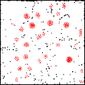
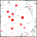
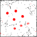
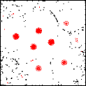
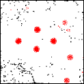
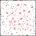
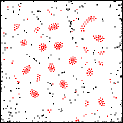
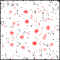
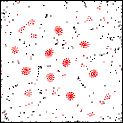
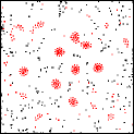
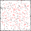
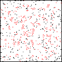
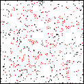
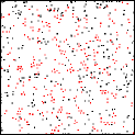
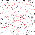
In order to take into account the diversified behaviours observed in nature, we now investigate the emergence of patterns considering different values of $\beta$ for each species ($\beta=0.5,0.125$ and $0.0625$). We start by considering null interaction between preys while the predators are able to feel their counterparts ($\beta_{predator}>0$ and $\beta_{prey}=0$). Observing the evolution of the system when three distinct values of $\beta_{predator}$ and $\alpha=32$ are considered (Fig. 4), we clearly identify the emergence of predator clusters which differ according to the $\beta_{predator}$ intensity.

When the attraction between predators is stronger (i.e. $\beta_{predator}=0.5$, see Figure 4-i), non-uniform clusters emerge in a few time steps (Fig. 4-i,a). Mutual attraction between different clusters progressively generates larger clusters, with the smaller clusters tending to be attracted by the larger ones (e.g., as is the case with the two clusters in the middle of Figure 4-i,a). Although the clusters present several shapes in the first steps, they evolve towards spherical shapes because of symmetrical internal forces and increase in the number of members (Fig. 4-i,b). After a transient, the number of clusters seems to stabilize. The smallest clusters can move throughout the space following the concentration of preys (Fig. 4-i,d) while the denser clusters repel strongly the preys. Consequently, the cluster net velocity becomes slower than that of the preys, allowing the latter to escape. As a consequence of the boundary conditions, such dense clusters tend to concentrate in the central region of $O$ while the preys move toward the periphery (Fig. 4-i,e). Therefore, we expect a resulting giant cluster of predators to appear after a long period of time.

(i)

(a) $t=10000$         (b) $t=75000$         (c) $t=150000$         (d) $t=300000$         (e) $t=500000$

(ii)

(a) $t=50000$         (b) $t=100000$         (c) $t=200000$         (d) $t=300000$         (e) $t=500000$

(iii)

(a) $t=100000$         (b) $t=200000$         (c) $t=300000$         (d) $t=400000$         (e) $t=500000$

Figure 4: Snapshots showing the pattern evolution of predators (red – on-line) and preys (black – on-line) when the attraction between predators is given by (i) $\beta_{predator}=0.5$, (ii) $\beta_{predator}=0.125$ and (iii) $\beta_{predator}=0.0625$.

Emergence of clusters also occur in the second configuration with $\beta_{predator}=0.125$ and $\beta_{prey}=0$ (Fig. 4-ii). However, they are visually more uniformly distributed (Fig. 4-ii,a) when compared with the previous configuration (Fig. 4-i,a). Since the attraction intensity is smaller, dense clusters emerge later along the dynamics (Fig. 4-ii,c) while the coarser clusters tend to be maintained along time (Fig. 4-ii,d). The last obtained time step (Fig. 4-ii,e) resembles the initial stage of the first configuration (Fig. 4-i,a), suggesting that the system would possibly evolve to a similar state. However, the giant cluster is not expected to emerge because of the weaker attraction between predators in this case.

The last snapshots sequence (Fig. 4-iii) presents the evolution when the lowest attraction intensity between predators is considered ($\beta_{predator}=0.0625$ and $\beta_{prey}=0$). In this configuration, we cannot identify dense clusters up to the last time step. However, spatio-temporal patterns of uniformly distributed small clusters emerge and evolve in a non-stationary way with predators and preys moving close to each other. The pattern consists of clusters with different sizes and shapes, indicating that predators are able to move throughout sub-space $O$, moving between clusters (Figs. 4-iii,d and 4-iii,e). Any attempt of escape by preys is promptly checked by predators, which can easily enclose any group of preys since the predators are not strongly attracted in this configuration.

When we consider null attraction between predators and different attraction intensities between preys, the spatio-temporal pattern tends to include uniformly distributed predators and preys (similar to Figure 3). Actually, small clusters of preys emerge but are readily eliminated because of the strong predators attraction, suggesting a cyclic process. Although we can identify some larger clusters with higher attraction intensity, the pattern is nearly independent of $\beta_{prey}$.

(i)

(a) $t=10000$         (b) $t=75000$         (c) $t=150000$         (d) $t=500000$

(ii)

(a) $t=50000$         (b) $t=100000$         (c) $t=200000$         (d) $t=500000$

Figure 5: Snapshots showing the evolving spatio-temporal patterns of predators (red – on-line) and preys (black – on-line). The attraction between same species individuals is given by (i) $\beta=0.5$ and (ii) $\beta=0.125$.

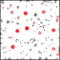
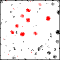
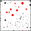
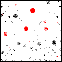
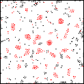
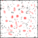
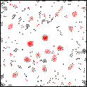
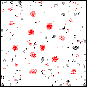
The last experiment consists in introducing attraction between individuals of both species, i.e., both predators and preys are able to feel their counterparts ($\beta_{predator}=\beta_{prey}=\beta>0$) while they can also feel each other (i.e. $\alpha=32$). The high level of attraction $\beta=0.5$ resulted a pattern of dense clusters of predators while smaller clusters of preys have also been observed along the first time steps (Fig. 5-i,a). The simultaneous attraction between members of each species generated distinct regions occupied by different species (Figs. 5-i,b to 5-i,d). The higher concentration of preys in some clusters increased the intensity of the sensitive field such that the clusters of predators could move around a larger region (following the prey clusters) when compared with the configuration with null attraction between preys (Fig. 4). The clusters of preys often disappear and emerge as a result of this attraction (Fig. 5-i). On the other hand, the clusters of predators become denser over time because of the non-uniformity in the distribution of the clusters of preys (Fig. 5-i,d). Since the preys are non-uniformly distributed in space, they create attractor regions.

The snapshots from Figure 5-ii show the evolution of the system with lower attraction $\beta=0.125$ between same species individuals. In this case, the clusters are not so dense and they are more uniformly spatially distributed (Fig. 5-ii,a). The preys are also organized in clusters of smaller sizes (Fig. 5-ii,b). The sequence of snapshots suggests a dynamical behaviour where some clusters aggregate more predators while the greatest part of clusters divide and recombine in new sets of animals (Fig. 5-ii,c). The clusters of predators follow the concentration of preys, which become higher in some regions over time.

In the last configuration where the attraction has the smallest value ($\beta=0.0625$), the density of clusters in the pattern was smaller than in the other cases (Figs. 5-i and 5-ii). Actually, the situation is similar to the absence of attraction between preys and small attraction between predators (Fig. 4-iii). However, in this case we could identify some small clusters of preys which constantly appeared and disappeared along time, while the clusters or predators resulted very small.

IV.2 Prey Elimination

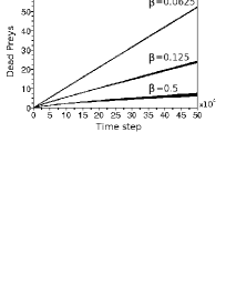
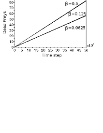
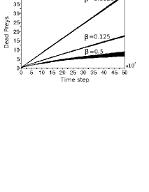
Spatial cluster structure emerges in animal behaviour as a consequence of several factors. Usually, group structure is a consequence of some type of similarity which provides protection against external agents. Protection not only against other individuals, but also against ideas and other cultural behaviour. In our model, the cluster structure depends on the attraction intensity between same species individuals and can favor species according to the attraction configuration. Although the preys death by itself is not necessarily the final purpose of our model, the number of eliminated preys indicates the importance of clusters and how they constrain the spatial movement of predators and preys. For instance, attraction between preys increases the sensitive field of predators because of the larger number of preys close one another. Consequently, the predators velocity directed to the prey clusters increases while the cluster structure constrains the movement of single preys. Contrariwise, the attraction between predators generates strong fields which allow preys to escape faster than the predators can move. This situation results in lower rates of preys deaths (Fig. 6-a), while preys were quickly eliminated in the previous case (Fig. 6-b).

(a) $\beta_{predator}>0\text{ and }\beta_{prey}=0$       (b) $\beta_{predator}=0\text{ and }\beta_{prey}>0$       (c) $\beta_{predator}>0\text{ and }\beta_{prey}>0$

Figure 6: Evolution of the amount of eliminated preys (average and standard deviations). We considered three intensities of attraction between same species animals.

The preys death rate is linear in almost all configurations, except in the cases with $\beta_{predator}=0.5$, where the growth rate is faster along the initial $200000$ time steps, slowing afterwards (Figs. 6-a and 6-c). This two-slope behaviour is a direct consequence of the emergence of dense predator clusters about this time step, decreasing the preys death rate. The existence of attraction in both species (Fig. 6-c) has similar effect as when attraction is allowed only between predators (Fig. 6-a). However, the cumulative number of eliminated preys is larger in the latter case (Fig. 6-a). These results suggest that the spatial organization of animals has crucial importance for their survival. Therefore, according to the predator species, there is no difference for preys to be organized in clusters or not. Since the hunting ability of predators is similar, the preys organization should be determined by other environmental reasons. In this sense, the choice of preys by predators might be directly related to the way in which the preys are spatially organized into groups.

V Structural Properties

The mechanism proposed to build the complex networks generates bi-partite networks with two types of nodes, respectively: predators and preys. Eliminating the connections between nodes of different types, two sub-networks are obtained which are henceforth named predator $\Gamma_{predator}$ and prey $\Gamma_{prey}$ networks. We shall analyse the enrollment and movement of individuals between spatial clusters by investigating local structural properties of both resulting networks.

V.1 Evolution of the structural properties

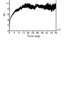
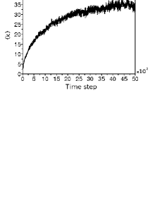
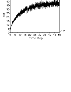
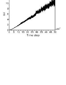
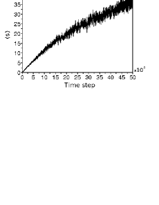
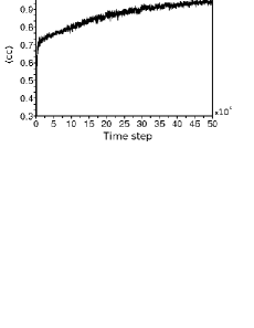
Considering the predator network $\Gamma_{predator}$. In the absence of attraction between preys ($\beta_{prey}=0$), the average degree $\langle k\rangle$ increases quickly within the $150000$ time steps, independently of the attraction intensity between predators (Fig. 7-i). After this stage, the average degree nearly stabilizes about $\langle k\rangle=8.5$ with $\beta_{predator}=0.5$ (Fig. 7-i,a). However, it exhibits a slower increase in the other configurations (Figs. 7-i,b and 7-i,c), suggesting that stabilization will also be eventually reached. Actually, because of the movements of predators between the spatial clusters, this measurement should stabilize after the network becomes completely connected. This will happen at $\langle k\rangle\sim 40$ in cases of $\beta_{predator}=0.125$ (Fig. 7-i,b) and of $\beta_{predator}=0.0625$ (Fig. 7-i,c), which corresponds nearly to the average number of spatial groups or number of nodes in the respective network $\Gamma_{predator}$ (the average value is obtained after an initial transient). Because the number of groups is smaller when $\beta_{predator}$ is larger, the threshold becomes smaller in that case (Fig. 7-i,a) and it possibly decrease whether the system converges to a giant component of predators.

(i)

(ii)

(iii)

(a) $\beta_{predator}=0.5$                   (b) $\beta_{predator}=0.125$                   (c) $\beta_{predator}=0.0625$

Figure 7: Evolution of the average structural properties in $\Gamma_{predator}$ when three intensities of attraction between predators and null attraction between preys are considered. (i) Average degree $\langle k\rangle$ ,(ii) Average strength $\langle s\rangle$ and (iii) Average clustering coefficient $\langle cc\rangle$. The standard deviation is shown to $50\%$ of the original values in cases (i) and (ii).

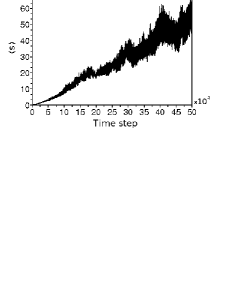
In the proposed growth method, the node strength relates to the history of proximity between a node and the members of its group, and inversely, to the rate of members exchanges between two spatial groups. The average strength $\langle s\rangle$ evolution seems to take place in stages when the attraction intensity between predators is larger ($\beta_{predator}=0.5$ – Fig. 7-ii,a). Possibly, the stages in which the growth rate is slower correspond to the intervals where the exchange rate between groups is small (Fig. 7-ii,a). Since the predators spend much time together, the weight $w_{\mu_{i},\mu_{j}}$ of connection $(\mu_{i},\mu_{j})$ in the network $\Gamma_{his}$ increases considerably and when two or more groups merge, the average strength suddenly rises. A lower attraction intensity implies on more circulation of predators in space and, consequently, constant association and disassociation to several groups. The level of proximity between predators tends to be smaller in the configuration with $\beta_{predator}=0.0625$ (Fig. 7-ii,c) when compared to the other two cases (Figs. 7-ii,a and 7-ii,b), where the predators movement is more constrained. As a consequence, in the last two cases, the predators spend more time together with the same partners. The larger strength in case of $\beta_{predator}=0.125$ is a consequence of the larger number of spatial groups (nodes of $\Gamma_{res}$).

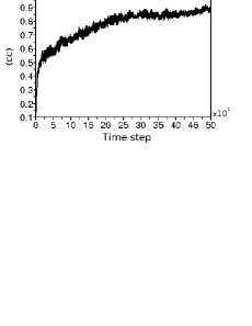
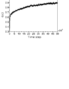
A smaller attraction intensity between predators implies in a faster increase in the average clustering coefficient $\langle cc\rangle$ within the first time steps (Fig. 7-iii). In the second growing stage (from nearly $25000$ to $250000$ time steps), the growth rate is higher for $\beta_{predator}=0.5$ (Fig. 7-iii,a). The latter effect is possibly a result of the decrease in the number of spatial groups in the first configuration (Fig. 4-i). Since the clustering coefficient measures the local connectivity (between common neighbours of a reference node), and the growth of $\langle cc\rangle$ (Fig. 7-iii) is higher than the growth of the corresponding $\langle k\rangle$ (Fig. 7-i), the connections occur mainly between nearby spatial groups. In other words, the movements required for following preys is considerable slow. A predator moves within a small Euclidean distance and then associates to one spatial group; after a while, the same or other predator moves again to another close spatial group in a non-stationary way.

Considering attraction between preys ($\beta_{prey}>0$) and null attraction between predators ($\beta_{predator}=0$), the structural properties of the evolution is similar to the situation with $\beta_{predator}=0.0625$ and $\beta_{prey}=0$, except for the configuration with $\beta_{prey}=0.5$. In that case, the stronger attraction of predators by dense clusters of preys implies on more movements of predators and, therefore, more connectivity between the nodes in comparison to the other two configurations. The absence of attraction between predators and the higher concentration of preys due to mutual attraction produces an overall behaviour where the predators have freedom to move throughout sub-space $O$. As a consequence, the average measurements values are slightly higher in this case in comparison to the situation with small attraction between predators (similarly to configuration of Figure 7-c), although presenting the same stages of evolution.

(a)                                             (b)                                             (c)

Figure 8: Evolution of $\Gamma_{predator}$ average structural properties when the attraction between same specie individuals is given by $\beta=0.5$. The standard deviation is shown to $50\%$ of the original values in (a) and (b).

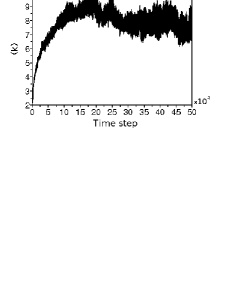
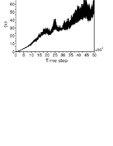
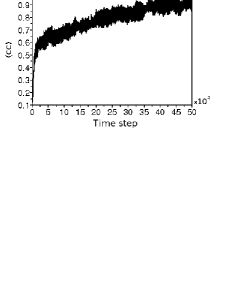
In the last experiment, involving attraction between predators ($\beta_{predator}>0$) and between preys ($\beta_{prey}>0$), the evolution of the average degree shows again an apparent stabilization in all cases. The number of nodes in the resulting network $\Gamma_{predator}$ (or number of connected components $\kappa$) is about $N\sim 9$ in the last time step observed (after a large transient). Since $N$ is higher than the plateau in the graph of Figure 8-a, the resulting network is not completely connected yet. We verified that at the maximum value (between $150000$ and $200000$ time steps), the number of spatial groups is approximately $1.5$ of the average degree value. Although the node average connectivity has decreased after this interval, the value increased if compared with the number of nodes in the network. This effect is related to the merging of clusters, which happens more frequently in the configuration where the attraction is higher (Fig. 5-i). This effect is not observed in the other two configurations, where the average number of groups is nearly constant (about $45$) over time and the curves are similar to the case in Figure 7-i. Comparing the number of nodes and the stabilization threshold, we observed that the resulting network is almost completely connected in the last time steps. The average connectivity among the nodes grows faster in the configuration with the smallest value of $\beta$ as a consequence of higher mobility. The average strength presented evolution similar to the first experiment (Fig. 7-ii). The main difference regards the stronger attraction between preys which generated clusters of preys. The non-existence of uniformly distributed preys implied in less movements between predator clusters due to absence of stimuli. Consequently, the strength values are higher (Fig. 8-b) when compared with the first experiment.

The decrease of the mobility between spatial groups is also observed by comparing the evolution of the clustering coefficient in Figure 8-c with Figure 7-iii,a. Once again, the clustering coefficient growth rate is very high within the first time steps (up to $10000$), maintaining a nearly constant growth henceforth. Actually, the evolution seems to stabilize after $t=450000$ in all configurations. Differently from the first experiment, the system may not evolve to a state where all nodes become connected. The effect is more probable in the configuration with $\beta=0.5$ provided the clusters do not merge in a single giant component. The movement of nodes between two clusters become less probable after a certain time step. This is a consequence of the fact that each cluster now has higher density and is considerably far from other clusters. The absence of stimuli because of prey clusters emergence and the mutual attraction inside the predator clusters also contributes to such a decrease of movements.

V.2 Strength Distribution

The average measurements provide global information about the complex network. However, the network internal structure can be completely different even when presenting similar average values Costa:review . The internal structure is responsible to constrain dynamical processes (e.g., cascade failures Motter:cascade ; Barabasi:review or epidemics Satorras:epidemic ; Newman:review ; Boccaletti:review ) in the network. Consequently, it is fundamental to characterize the resulting network in terms of measurements related to their internal topological properties.

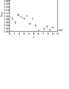
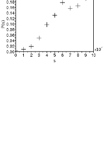
The strength distributions (histograms) have different shapes in the three resulting networks (Fig. 9) when we consider attraction between predators ($\beta_{predator}>0$) and null attraction between preys ($\beta_{prey}=0$). Although the configuration with $\beta_{predator}=0.5$ (Fig. 9-a) presents undefined shape, we see that the maximum strength increases considerable between $100000$ and $300000$ time steps. The number of nodes with large strength values also increases at the next time steps considered (Fig. 9-iii,a), indicating that the mobility between groups decreases with time, which can be seen by the existence of nearly stationary (in shape and number of members), dense spatial clusters in Figure 4. Contrariwise, the other two configurations (Figs. 9-b and 9-c) present a Gaussian-like strength distribution with a characteristic scale given by the average value (the average can be verified by comparison with graphs of Figure 7-ii). Although presenting a characteristic membership permanence time, some individuals constantly change between their respective groups (decreasing the strength), while others associate in a group for a long time (increasing the strength) and barely move between different groups. The predators in the last case can be seen as the core of the group, since they spent much time together and are responsible for maintaining the group united.

(i)

(ii)

(iii)

(a) $\beta_{predator}=0.5$                   (b) $\beta_{predator}=0.125$                   (c) $\beta_{predator}=0.0625$

Figure 9: Strength distribution for predator networks at three time steps: (i) $t=100000$, (ii) $t=300000$ and (iii) $t=500000$. We consider three attraction intensities between same-specie individuals.

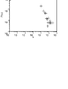
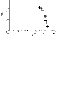
In the case of the prey network $\Gamma_{prey}$, the strength distribution (Fig. 10) resulted in a completely different function when compared to the predator network (Fig. 9-iii). In this case the histograms remind a power law function (especially along the largest values) with the maximum strength value being larger in case of larger $\beta_{predator}$ (Fig. 10-a) and the other two configurations apparently presenting two-slopes (Figs. 10-b and 10-c). The shape of the function suggests that the system converged to an organized state. In the last time step considered, few preys stayed together for a long time (higher strength), while their majority moved away or died frequently (lower strength), such that the emergent distribution is scale-free-like (Observe the high number of null strength nodes). Although a low strength value could indicate a high rate of changes between groups, the low values observed in the preys network is mainly because of preys deaths since the maximum strength value is much larger in the predators network and the amount of eliminated preys decreases with larger $\beta_{predator}$ (Fig. 6-a), while the maximum strength value increases for larger $\beta_{predator}$ (Fig. 10).

(a) $\beta_{predator}=0.5$                   (b) $\beta_{predator}=0.125$                   (c) $\beta_{predator}=0.0625$

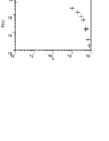
Figure 10: Strength distribution for $\Gamma_{prey}$ at $t=500000$ when three intensities of attraction are considered between predators.

Null attraction between predators ($\beta_{predator}=0$) and attraction between preys ($\beta_{prey}>0$) generated a similar pattern as in the case with $\beta_{predator}=0.125$ and $\beta_{prey}=0$, though exhibiting a Gaussian-like strength distribution. Comparing with the case when only attraction between predators is considered (Fig. 9-c), we verified that the maximum strength is considerably higher at the same time step observed in that case. It suggests more movements between groups in the configuration with $\beta_{prey}>0$ and $\beta_{predator}=0$ because of the stronger attraction provided by the high concentration of preys. Once again, the prey elimination mechanism implies in short life-time for preys and consequently, suggesting a power law distribution along the highest values.

In the last experiment, considering attraction between same species individuals, the strength distributions present some interesting effects. The configuration with larger $\beta$ converged to a power law-like distribution (Fig. 11-a) due to formation of dense prey clusters which implied in faster predator clusters emergence in some regions of the space. Dense predator clusters have strong attraction fields and therefore, any predator close to them is readily attracted and barely escapes from the cluster. Consequently, only small groups change individuals frequently. In case of $\beta=0.125$, the system evolves from a Poisson-like state to a combination of Gaussian-like on the left with a power-law-like on the right (Fig. 11-b). At last, $\beta=0.0625$ (Fig. 11-c) is similar to the cases with small (Fig. 9-c) or null attraction between predators, suggesting that a reasonably weak attraction intensity will result in the same non-stationary state. In other words, weak attraction between predators and/or between preys does not produce different collective behaviour in the system.

(a) $\beta=0.5$                            (b) $\beta=0.125$                            (c) $\beta=0.0625$

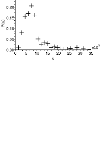
Figure 11: Strength distribution for $\Gamma_{predator}$ at $t=500000$ when three attraction intensities between same specie individuals are considered.

The power law-like distribution is observed in the prey network $\Gamma_{prey}$ for large values as in the other configurations (Fig. 12). The effect confirmed the hypothesis that such a scale-free structure emerged because of the elimination of preys and not because of the attraction mechanism between two individuals. The longer life-time of preys is identified by the larger maximum strength observed in this case in comparison to the other configurations (Fig. 10).

(a) $\beta=0.5$                            (b) $\beta=0.125$                            (c) $\beta=0.0625$

Figure 12: Strength distribution for $\Gamma_{prey}$ at $t=500000$ with three attraction intensities between same species individuals.

$\beta_{Predator}$$\beta_{Presa}$	0	0.0625	0.125	0.5
0	No clusters	Clusters of predatorsPredator:“Gaussian”Prey:Two-regime “Power-law”	Dense clusters of predatorsPredator:“Gaussian”Prey:“Two-regime Power-law”	Dense clusters of predatorsPredator:Unidentified shapePrey:“Power-law”
0.0625	Some small clustersPredator:“Gaussian”Prey:“Power-law”	Clusters of predators and small clusters of preysPredator:“Gaussian”Prey:“Power-law”
0.125	Small clustersPredator: “Gaussian”Prey:“Power-law”		Some dense clusters of predators and clusters of preysPredator:“Gaussian”/“Power-law”Prey:“Power-law”
0.5	Small clusters of preysPredator:“Gaussian”Prey:“Power-law”			Dense clusters of predators and some dense dense clusters of preysPredator:“Power-law”Prey:“Power-law”

Table 1: Summary of the main properties (spatial and topological) according to different attraction intensities between same species individuals.

V.3 Clustering Coefficient Distribution

The clustering coefficients have nearly the same distribution in all considered configurations for the predator network (Fig. 13). The only difference is observed at the scale of the distributions since smaller $\beta_{predator}$ implies more movement and, consequently, faster connections between groups. The normalized distributions become narrower and present characteristic scales which move to the right over time, indicating that all groups will become connected after a long period of time. The shapes of the curves indicate that higher attraction between predators constrains the movement and postpones creation of triangles between common neighbours of a reference node. In case of weaker attraction, predators are able to move between groups and consequently, the amount of nodes with larger clustering coefficient becomes higher (Fig. 13-c). Although the number of nodes with higher clustering coefficient constantly increases over time, there are many nodes with small values of $cc$ for larger $\beta_{predator}$ (Fig. 13-a).

(i)

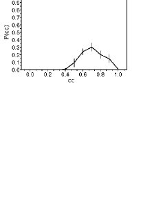
(ii)

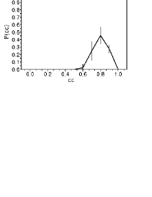
(iii)

(a) $\beta_{predator}=0.5$                   (b) $\beta_{predator}=0.125$                   (c) $\beta_{predator}=0.0625$

Figure 13: Clustering coefficient distribution for $\Gamma_{predator}$ at three time steps: (i) $t=100000$, (ii) $t=300000$ and (iii) $t=500000$. We consider three attraction intensities between predators.

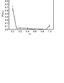
In the preys network $\Gamma_{prey}$, all configurations resulted in a clustering coefficient distribution with a clear division (Fig. 14), which suggests the existence of two distinct states in the system (nearly constant over time). A large number of preys has small connectivity in their neighbourhood while a small number presents a high level of local connectivity among its neighbours. A small clustering coefficient is a consequence of two effects: complete absence of movement or a high death rate, which avoid triangle formation. Since the frequency of $cc$ null values increases as we decrease the attraction between predators (Fig. 14), we conclude that the main fact behind this effect is exactly the death of preys. As shown before, such deaths increase as $\beta_{predator}$ decreases (Fig. 6-a). In case of attraction between preys, the effect is the opposite, i.e. the number of dead preys and of nodes (predator groups) with null $cc$ increases with $\beta_{prey}$. Since the configuration with $\beta_{prey}=0.5$ has regions with high concentration of preys, which are not completely static and are not eliminated frequently too, the probability to establish closed triangles increases and explains the higher frequency observed at the maximum value of $cc$ ($cc=1$). The existence of groups with maximum clustering coefficient indicates that some preys stay a long time in the system and, although they are eliminated, other preys keep some spatial groups united and permit triangle formation (about $10\%$ of the nodes in $\Gamma_{prey}$). With attraction between same species individuals, we observed a higher frequency of intermediate clustering coefficient values. The existence of clusters in both species resulted in extended life-time for the preys, which allowed more movement and connections between nearby spatial groups.

(a) $\beta_{predator}=0.5$                   (b) $\beta_{predator}=0.125$                   (c) $\beta_{predator}=0.0625$

Figure 14: Clustering coefficient distribution at $t=500000$ for $\Gamma_{prey}$ when three intensities of attraction between predators are considered.

VI Conclusions

The current paper has focused on multiple networks systems involving interacting species. Since the system was originally motivated by ecology, we assumed that preys are eliminated when they move sufficiently close to a predator, but new preys are randomly displaced in the system in order to replace those which are consumed. Spatio-temporal clusters emerge from the dynamics, which involves movements of individual between clusters. Two complex networks containing the same set of nodes are considered. In one network, the weights represented the Euclidean distances between two individuals. In the other network, the number of steps during which two individuals were close enough are considered as weights. By merging both networks, we obtained a third complex network whose nodes represented spatial groups defined by the connected sub-networks. Such a growth mechanism implied the connections to incorporate information about the history of the individuals movement.

Several configurations, defined in terms of the intensity of the attractions between preys and predators, were considered in our simulations. The increase in the attraction between same species individuals generated dense clusters whose sizes and shapes were a result of the same species attraction intensity as well as the other species attraction features. Dense predator clusters constrained the movement of single predators, while dense prey clusters generated strong fields and attracted many predators. As a consequence, the rate of eliminated preys was higher when the preys were organized into clusters and predators had null attraction between them. We have observed that group organization could benefit the species according to the intensity of intra-species attraction. On the other hand, some configurations (with small attraction) evolved to states where the group organization had few or no advantage to any of the two species.

By using the complex network theory, we observed that the average degree of the resulting predator network increased up to a threshold corresponding to the number of spatial groups, i.e., the system evolved to a fully connected state. Since the average clustering coefficient increased faster than the average degree, we concluded that members exchanges between nearby spatial groups were more frequent than between far away groups. The analysis at the last time step showed that the system converged to an organized state. The predator network presented a Gaussian-like strength and clustering coefficient distributions in nearly all configurations while approximately scale-free strength and a polarized clustering coefficient distributions emerged in the case of the preys network. The prey elimination mechanism was responsible for generating the observed structure in the prey network. Since preys are eliminated frequently, they are not able to move long enough throughout space and establish connections between all clusters, as was the case with the predators.

In order to further investigate the model, we propose the following future developments: (i) study of the effect of individuals density and other scale properties of the system, (ii) investigation of clusters emergence when considering other attraction functions and more species interacting together, (iii) analysis of collective phenomena (e.g., epidemics and opinion formation as a result of dynamical propagation of diseases and ideas from specific individuals), and finally (iv) application of the same methodology in empirical data, for example, to study the movement of animals in the field.