Constraining Dark Energy Anisotropic Stress

Abstract

We investigate the possibility of using cosmological observations to probe and constrain an imperfect dark energy fluid. We consider a general parameterization of the dark energy component accounting for an equation of state, speed of sound and viscosity. We use present and future data from the cosmic microwave background radiation (CMB), large scale structures and supernovae type Ia. We find that both the speed of sound and viscosity parameters are difficult to nail down with the present cosmological data. Also, we argue that it will be hard to improve the constraints significantly with future CMB data sets. The implication is that a perfect fluid description might ultimately turn out to be a phenomenologically sufficient description of all the observational consequences of dark energy. The fundamental lesson is however that even then one cannot exclude, by appealing to observational evidence alone, the possibility of imperfectness in dark energy.

1 Introduction

The observed accelerated expansion of the universe (see e.g.(Astier et al., 2006)) is usually ascribed to the existence of a cosmic fluid with a negative pressure comparable to its small but cosmologically significant energy density. While numerous possible origins have been proposed for this dark energy (see (Copeland et al., 2006) for a review) most of them are variations of the cosmological constant or the scalar field scenario (Wetterich, 1988). These include several different kinds of couplings to matter (baryons, neutrinos, cold dark matter(Amendola, 2000; Brookfield et al., 2006; Mota & Shaw, 2007, 2006; Koivisto, 2005)), couplings to gravity (the curvature scalar, Lovelock invariants, etc (Koivisto & Mota, 2007b, c)), and also non-canonical kinetic terms (phantoms, tachyons, K-essence, etc (Gibbons, 2002; Armendariz-Picon et al., 2001)). With such a zoo of models, it is important to investigate, and search for, some particular feature or property of dark energy, which could be used to rule out some of (or at least distinguish among) all these possibilities.

It is already well known in the literature that to discriminate between different classes of models, it is not sufficient to consider just the background expansion. One has also to study the evolution of cosmological perturbations. General Relativity dictates that any component with its equation of state $w\neq-1$, where $w=-1$ corresponds to the cosmological constant, must fluctuate. Therefore a generic dark energy component has perturbations which couple to matter perturbations. These however can be small, since if one has $w\approx-1$, the component can be nearly smooth, and if the Jeans length of dark energy is large, its perturbations may be confined to very large scales only. This is typical for the usual minimally coupled quintessence models, since their sound speed of perturbations, $c^{2}_{lam}$, is equal to the light speed, $c^{2}_{lam}=1$, which sets a large Jeans length (Bean & Dore, 2004; Xia et al., 2007). However, for some other dark energy candidates that is not the case (Mota & van de Bruck, 2004; Bagla et al., 2003; Bento et al., 2002), and such feature might help to differentiate between these classes of models.

In addition to the $w$ and $c^{2}_{lam}$, there is an important characteristic of a general cosmic fluid which is its anisotropic stress $\sigma$ (Hu, 1998). This vanishes for a minimally coupled scalar field and perfect fluid candidates, but is a generic property of realistic fluids with finite shear viscous coefficients (Schimd et al., 2006; Brevik et al., 2004; Nojiri & Odintsov, 2005). Basically, while $w$ and $c^{2}_{lam}$ determine respectively the background and perturbative pressure of the fluid that is rotationally invariant, $\sigma$ quantifies how much the pressure of the fluid varies with direction. In fact the anisotropic stress perturbation is crucial to the understanding of evolution of inhomogeneities in the early, radiation dominated universe (Hu, 1998; Koivisto & Mota, 2006). Therefore an obviously interesting question is whether present observational data could allow for an anisotropic stress perturbation in the late universe which is dominated by the mysterious dark energy fluid (Ichiki & Takahashi, 2007; Barrow, 1997).

The cosmological effects of $\sigma$ due to possible viscosity of dark energy are however quite neglected in the literature. The main reason for disregarding the anisotropic stress in the dark energy fluid might be that conventional dark energy candidates, such as the cosmological constant or canonical scalar fields, are perfect fluids with $\sigma=0$. However, since there is no fundamental theoretical model to describe dark energy, there are no strong reasons to stick to such assumption. Moreover, coupled scalar fields have indeed a non-negligible anisotropic stress(Schimd et al., 2006), and dark energy vector field candidates (which have been proposed in (Armendariz-Picon, 2004; Kiselev, 2004; Zimdahl et al., 2001)) also have $\sigma\neq 0$.

The aim of the present paper is to investigate the potential cosmological signatures of a very general dark energy component, which is characterize by an equation of state, sound speed and anisotropic stress. In section 2 we review the parameterization of a generalized cosmological fluid and comment its relation to some recent studies of anisotropies dark energy. The parameterization will then be subjected to the most detailed and most extensive scrutiny this far. The data and method utilized for this are described in section 3. In the section 4 we use the most recent cosmological data to constrain the properties of dark energy. Section 5 is devoted to investigate how much the future data could be able to improve the constraints. We conclude by stating the fundamental uncertainty in the properties of dark energy but also mention some cases where a positive detection could be established.

2 Dark energy stress parameterization

Consider a general fluid with the energy momentum tensor

$$\mbox{$$}T_{\mu\nu}=\rho u_{\mu}u_{\nu}+ph_{\mu\nu}+\Sigma_{\mu\nu},$$ (1)

where $u_{\mu}$ is the four-velocity of the fluid, and the projection tensor $h_{\mu\nu}$ is defined as $h_{\mu\nu}\equiv g_{\mu\nu}+u_{\mu}u_{\nu}$. Here $\Sigma_{\mu\nu}$ can include only spatial inhomogeneity. At the background level, the evolution of the fluid is determined by the continuity equation,

$$\mbox{$$}\dot{\rho}+3H(1+w)\rho=0.$$ (2)

The effects to the overall expansion are therefore determined by the equation of state $w$ alone. We define a perfect fluid by the condition $\Sigma_{\mu\nu}=0$. The condition for the adiabaticity of a fluid is $p=p(\rho)$, which implies that the evolution of the sound speed is determined by the equation of state alone. Generally, however, the sound speed is defined as the ratio of pressure and density perturbations in the frame comoving with the dark energy fluid (Weller & Lewis, 2003),

$$\mbox{$$}c^{2}_{lam}\equiv\frac{\delta p}{\delta\rho}_{|{de}}.$$ (3)

In the adiabatic situation one has $c^{2}_{lam}=dp/d\rho=\frac{\dot{p}}{\dot{\rho}}=w-\frac{\dot{w}}{3H(1+w)}$, but in general the sound speed is an independent variable. In the following we will consider a constant equation of state for simplicity.

Taking these considerations into account, the evolution equations for the dark energy density perturbation $\delta$ and velocity potential $\theta$ in the synchronous gauge (Ma & Bertschinger, 1995), can be written as

$$\mbox{$$}\dot{\delta} = -(1+w)\left\{\left[k^{2}+9H^{2}(c^{2}_{lam}-w)\right]\frac{\theta}{k^{2}}+\frac{\dot{h}}{2}\right\}$$ (4)

$$- 3H(c^{2}_{lam}-w)\delta,$$

$$\mbox{$$}\dot{\theta}=-H(1-3c^{2}_{lam})\theta+\frac{c^{2}_{lam}k^{2}}{1+w}\delta-k^{2}\sigma,$$ (5)

where $h$ is the trace of the synchronous metric perturbation. Here $\sigma$ is the anisotropic stress of dark energy, related to notation of Eq.(1) by $(\rho+p)\sigma\equiv-(\hat{k}_{i}\hat{k}_{j}-\frac{1}{3}\delta_{ij})\Sigma^{ij}$. From the above equations it is then clear that, while $w$ and $c^{2}_{lam}$ determine respectively the background and perturbative pressure of the fluid that is rotationally invariant, $\sigma$ quantifies how much the pressure of the fluid varies with direction.

To close the system of equations, we describe the evolution of the anisotropic stress with an equation adopted from Hu (Hu, 1998),

$$\mbox{$$}\dot{\sigma}+3H\sigma=\frac{8}{3}\frac{c^{2}_{vis}}{1+w}(\theta+\frac{\dot{h}}{2}+3\dot{\eta}).$$ (6)

This parameterization leads to reasonable results and approximates the evolution of any fluid present in the standard cosmological model, in particular neutrinos and photons which have a non-zero anisotropic stress (Hu & Eisenstein, 1999). More specifically, for those relativistic components, the correct choice for the viscous parameter is $c^{2}_{vis}=1/3$. A perfect fluid (vanishing shear viscosity) should have $c^{2}_{vis}=0$.

Equivalently, one can describe the physical properties of $\sigma$ by introducing the rescaled parameter $\alpha_{vis}=c^{2}_{vis}/(1+w)$. While $c^{2}_{vis}$ is somehow physically analogous to sound speed squared, the $\alpha_{vis}$ is the quantity directly multiplying the source term of the stress (see RHS of eq. (6)). In this study we will use both the $c^{2}_{vis}$ and $\alpha_{vis}$ parameterizations. Since $w$ is constrained near $w=-1$, where the relation between these parameters is divergent, using one or the other might lead to different results and interpretations. The statistical details also depend on which parameter one assumes a uniform distribution, and it is useful to test how robust ones conclusions are to such assumptions.

Usually, a dark energy fluid with nonzero $\alpha_{vis}$ generates shear stress which tends to smoothen its distribution. However, the consequences to phantom dark energy are qualitatively different and for such a fluid, with $w<-1$, a shear stress drives the clustering. With negative $\alpha_{vis}$, exponential growth is typical for all kinds of dark energy. In the case of positive $\alpha_{vis}$, and constant $w$ and $c^{2}_{lam}$, the effects are confined to superhorizon scales and typically small (Koivisto & Mota, 2006). This is in contrast to anisotropic stress which originates from modifications of the gravity sector or quintessence couplings, since they typically modify the gravitational potentials at small scales. A recent study by Amendola et al (Amendola et al., 2004) considers the possibility of using weak lensing to obtain limits on the dark energy parameters motivated partially by modified gravity (Amendola et al., 2004). Our study can be considered as an exploration of complementary aspects since the effects we encounter, occur (except for negative $c^{2}_{lam}$ or $\alpha_{vis}$) at some orders of magnitude larger scales than those possible to probe with weak lensing experiments. An interesting approach is also that of Caldwell et al (Caldwell et al., 2003) who, parameterizing directly the deviation from the general relativistic perfect fluid metric, and assuming it to depend on the amount of dark energy, find that this assumption leads to relatively weak constraints on cosmological scales, whereas the bounds on the solar system are known to be tight.

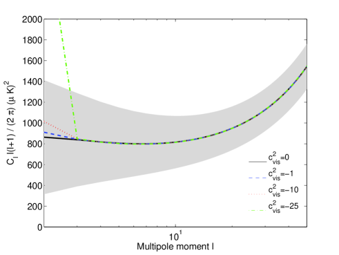
Figure 1: The CMB temperature power spectrum for models with different values of $w$ and $c^{2}_{vis}$. The upper panel is for a model with $w=-1.2$ and $c^{2}_{vis}\leq 0$, while the lower panel shows the results for a model with $w=-0.8$ and $c^{2}_{vis}\geq 0$. The grey shading indicates the cosmic variance around the models with $c^{2}_{vis}=0$. All models plotted here have $c^{2}_{lam}=1$.

To illustrate the effect of $c^{2}_{vis}$ on the CMB power spectrum, we have in Figure 1 shown the CMB temperature power spectra for models with different values of $w$ and $c^{2}_{vis}$. In models with $w=-1.2$, one sees that the deviation from the $c^{2}_{vis}=0$ model starts to become significant with $c^{2}_{vis}=-25$. With $w=-0.8$, the deviations remain small, even with $c^{2}_{vis}=1000$. From this we would expect that it is possible to find some lower limit on $c^{2}_{vis}$ in models with $w<-1$, while it will be difficult to find upper limits on $c^{2}_{vis}$ in models with $w>-1$.

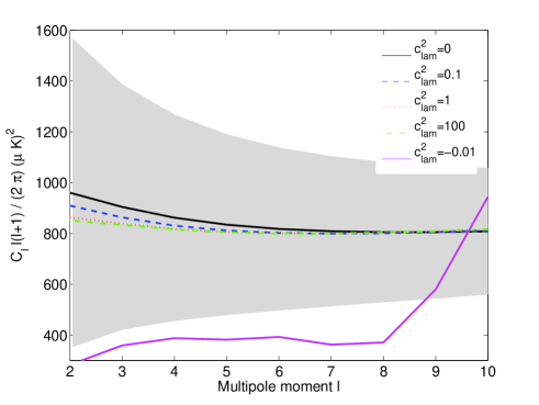
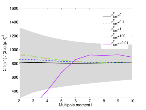
Figure 2: The CMB temperature power spectrum for models with different values of $w$ and $c^{2}_{lam}$. The upper panel shows the results for a model with $w=-1.2$, while the lower panel shows models with $w=-0.8$. The grey shading indicates the cosmic variance. All models shown here $c^{2}_{vis}=0$.

In Figure 2 we have plotted the CMB temperature power spectra for models with different values of $w$ and $c^{2}_{lam}$. We see that for values of $c^{2}_{lam}$ increasing over $c^{2}_{lam}=1$, the shape of the power spectra seems to stabilize, even when $c^{2}_{lam}$ gets as large as $c^{2}_{lam}=100$. So also in the case of $c^{2}_{lam}>0$ it looks difficult to distinguish between the different models. Such difficulty can be understood noticing that, increasing $c^{2}_{lam}$ will lead to a smoothening of a quintessence-like case. This is itself already almost smooth. Therefore we do not see much difference even when $c^{2}_{lam}=100$. Notice, however, that negative $c^{2}_{lam}$ is also conceivable, and it corresponds to gravitational instability. This leads to the clustering of dark energy and thus to possibly observable effects. In Figure 2 we see that the observable effect of $c^{2}_{lam}<0$ is much more evident than for $c^{2}_{lam}>0$. Such possibility will also be investigated in the following sections.

3 Data and methods

In our analysis we use data from observations of the anisotropies of the Cosmic Microwave Background, the distribution of large scale structures (LSS), the distance-redshift relation from type Ia supernovae (SNIa), and an additional prior on the Hubble parameter. The parameter estimation analysis is done using a modified version of the Markov chain Monte Carlo code CosmoMC (Lewis & Bridle, 2002).

In our basic cosmological model, we assume a flat, homogeneous and isotropic background spacetime, and a simple power law primordial power spectrum. Thus, we allow the six parameters $\{\Omega_{b}h^{2},\Omega_{m},\log(10^{10}A_{S}),h,n_{s},\tau\}$ to vary freely. Here $\Omega_{i}$ is the ratio of the energy component $i$ to the critical density today, $A_{S}$ is the amplitude of the primordial power spectrum, $h$ is the dimensionless Hubble parameter today, $n_{s}$ is the scalar spectral index and $\tau$ is the optical depth at recombination. The exact definitions of the parameters are given by the CosmoMC code. In addition to these basic six parameters we have also studied changes in $w$, $c^{2}_{vis}$ (or $\alpha_{vis}$) and $c^{2}_{lam}$.

The most constraining CMB dataset at present is the 3-year data release from the WMAP team. In our analysis we have used both the temperature (Hinshaw et al., 2007) and polarization (Page et al., 2007) data from this experiment together with the likelihood code provided by the WMAP team . Since the effects we are studying here are most prominent on large angular scales in the CMB signal, we do not take additional small-scale CMB experiments into account in this analysis.

In one case we have also utilized LSS data from the Sloan Digital Sky Survey Luminous Red Galaxy Sample (SDSS-LRG) (Tegmark et al., 2006). When using information on SNIa distance-redshift relation, we use data from the Supernova Legacy Survey (SNLS) (Astier et al., 2006).

We have also used a prior of $h=0.72\pm 0.08$ from the Hubble Space Telescope Key Project (HST) (Freedman et al., 2001) and a top-hat prior on the age of the universe, 10Gyr$<$Age$<$20Gyr, throughout the entire analysis.

4 Constraints from present data

4.1 Constraining dark energy viscosity

To start with we have used the $c^{2}_{vis}$ parameterization, looking at two distinct scenarios. In one case we have $\{w>-1,c^{2}_{vis}>0\}$, and in the other case $\{w<-1,c^{2}_{vis}<0\}$. Here, and for the rest of subsection 4.1, we have set $c^{2}_{lam}=1$.

In Figure 3 we show the 65% and 98% confidence level (CL) contours in the $w-c^{2}_{vis}$ plane for the two main scenarios mentioned above. We see that in the first case there is no clear degeneracy between $c^{2}_{vis}$ and $w$, and we find no upper limit on $c^{2}_{vis}$ here. This is exactly what we would expect from an inspection of Figure 1; when $\{w>-1,c^{2}_{vis}>0\}$, the effects of varying $c^{2}_{vis}$ are negligible.

For the latter case, where $w<-1$ and $c^{2}_{vis}<0$, we do however find a degeneracy between these parameters, and in this case we also find lower limits on $c^{2}_{vis}$. Using only WMAP data we find $c^{2}_{vis}>-19.5$ at 95% confidence level (CL) from the 1 dimensional distribution of $c^{2}_{vis}$. Since there are observable effects of a non-zero $c^{2}_{vis}$ in this scenario, we also tried to add SDSS-LRG and SNLS data to see if this would improve our constraints on $c^{2}_{vis}$. In this case the lower limit on $c^{2}_{vis}$ becomes $c^{2}_{vis}>-24.9$ at 95% CL. We can also easily see from the figure that adding SDSS-LRG and SNLS data does not improve the limits on $c^{2}_{vis}$, only on $w$. The reason is that the effects of $c^{2}_{vis}$ occur at larger scales than probed by the SDSS-LRG. Therefore this additional data would only be interesting if it could break degeneracies between $c^{2}_{vis}$ and other parameters that govern the shape of the power spectrum for low $l$s. We see from Figure 1 that although we do have a degeneracy between $c^{2}_{vis}$ and $w$, the limits on $c^{2}_{vis}$ would only be improved by some data set that would favor a $w<-1$.

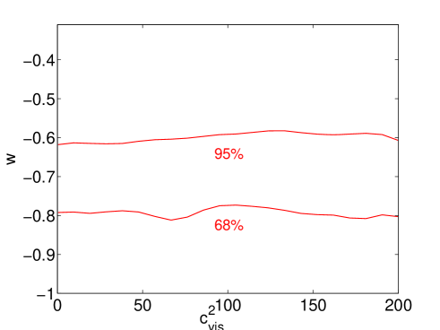
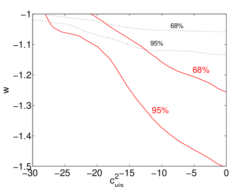
Figure 3: 68% and 95% contours of $c^{2}_{vis}$ and $w$. In the upper panel $w>-1$ and $c^{2}_{vis}>0$, while in the lower panel $w<-1$ and $c^{2}_{vis}<0$. We see that the constraints are much tighter for negative $c^{2}_{vis}$ than for positive. In the right plot we have also shown how the constraints improve when including SDSS-LRG and SNLS data (dotted black contours). In these models $c^{2}_{lam}=1$.

Next, we turn to the $\alpha_{vis}$ parameterization. To constrain this parameter we focus on a model where $\alpha_{vis}<0$, since we find no upper limits on a positive $\alpha_{vis}$. In Figure 4 we show the 65% and 98% CL contours for $w$ and $\alpha_{vis}$ in this model. We see that $\alpha_{vis}$ is bounded from below and that values of $\alpha_{vis}$ slightly below zero are allowed. In this case we find that $\alpha_{vis}>-0.23$ at 95% CL.

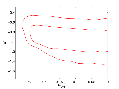
Figure 4: 68% and 95% contours of $\alpha_{vis}$ and $w$. We see that slightly negative values of $\alpha_{vis}$ are allowed, and that the allowed values for $\alpha_{vis}$ in this parameter range has only a weak dependence on $w$. In this model $c^{2}_{lam}=1$.

Since we got a lower limit on $c^{2}_{vis}$ when having $w<-1$, we would also expect to find an upper limit on $\alpha_{vis}$ in this case. In Figure 5 we show the 1 dimensional marginalized likelihood for $\log\alpha_{vis}$ for a model with $w=-1.2$. We find that $\log\alpha_{vis}<3.2$ at 95% CL ($\alpha_{vis}<24.5$), which corresponds well to the limits we found for $c^{2}_{vis}$ with $w<-1$.

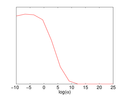
Figure 5: Marginalized probability distribution for $\log(\alpha_{vis})$ for a model with $w=-1.2$ and $c^{2}_{lam}=1$.

4.2 Constraining dark energy sound speed

In this section we investigate what constraints can be put in the dark energy sound speed, $c^{2}_{lam}$, from WMAP data. Throughout this subsection $\alpha_{vis}=0$.

From Figure 2 we see that the effect of varying $c^{2}_{lam}$ away from $c^{2}_{lam}=1$ is negligible for models with $c^{2}_{lam}>1$, but notable when varying $c^{2}_{lam}$ in the regime $c^{2}_{lam}<1$. Thus we would expect to find a lower limit, but not an upper limit on the value of $c^{2}_{lam}$, and this is indeed the case.

In Figure 6 we have plotted the 2-dimensional confidence contours in the $c^{2}_{lam}-w$ and $c^{2}_{lam}-\Omega_{m}$ planes that we get from the WMAP data and for a model where $c^{2}_{lam}$ is allowed to vary freely in the interval $\{-20,20\}$. In both cases we see that we do get a lower limit, and also that there is hardly any degeneracy between $c^{2}_{lam}$ and these parameters (or any of the other parameters in our model). Therefore, as in the case of $c^{2}_{vis}$ and $\alpha_{vis}$, we would not expect to improve our constraints on $c^{2}_{lam}$ by using other types of cosmological data.

Note that the intuitively plausible models with $c^{2}_{lam}=0$ reside at the lower end of a long “ridge” of $c^{2}_{lam}$ values that fit the data almost equally well. Therefore the interpretation of the confidence contours should be done with some care. This is the reason why we do not state any lower limit on $c^{2}_{lam}$ here. Also note that the shaded backgrounds in Figure 6 refer to the mean likelihood of the samples, whereas the contours show the marginalized likelihoods. For such highly non-gaussian distribution that we have here, there is a significant mismatch between these. See Appendix C in (Lewis & Bridle, 2002) for a discussion on this.

In Figure 7 we show the marginalized probability distribution of $c^{2}_{lam}$ for the same model. In the figure we have also indicated the mean likelihoods of the samples by the background shading color. Here we clearly see the effect of the converging power spectrum for $c^{2}_{lam}>1$, as the likelihood for models with $c^{2}_{lam}>1$ does not decrease. We also see that we are allowed to have models with $c^{2}_{lam}$ slightly negative, but that the models rapidly become incompatible with the data for $c^{2}_{lam}<0$.

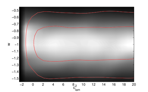
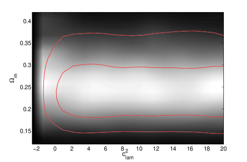
Figure 6: 68% and 95% confidence contours in the $c^{2}_{lam}$-$w$ and $c^{2}_{lam}$-$\Omega_{m}$ planes using WMAP data. We see that the degeneracies between $c^{2}_{lam}$ and both these parameters are very weak. The colored background indicates the mean likelihoods of the samples. In this model $\alpha_{vis}=0$.

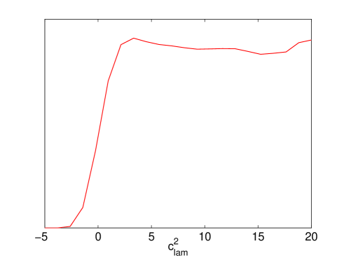
Figure 7: The marginalized probability distribution for $c^{2}_{lam}$ using WMAP data. No upper limit is obtained. In this model $\alpha_{vis}=0$ and $w$ is allowed to vary freely.

4.3 Effect on other parameters

Another interesting issue is whether the extra freedom in the dark energy fluid will affect the constraints on the other parameters in our cosmological model. That is, are the parameter constraints in the $\Lambda$CDM model robust to changes in $c^{2}_{vis}$ and $c^{2}_{lam}$. This was also studied in (Ichiki & Takahashi, 2007), where they found that $\alpha_{vis}$ did not change the constraints in the other cosmological parameters significantly, but that varying $c^{2}_{lam}$ shifted the other parameter ranges slightly.

In Figure 8 we have plotted the marginalized likelihoods for different cosmological parameters in the case of a 7 parameter model with free $w$ but with $\alpha_{vis}=0$ and $c^{2}_{lam}=1$. We compare this to a model where $\alpha_{vis}$ is allowed to vary freely in the interval $\{-20,20\}$ (the same model as shown in Figure 4). Also shown is a model with $\alpha_{vis}=0$ and $c^{2}_{lam}=0$. We see that the extra freedom in the $\alpha_{vis}$ parameter does not change the other parameter distributions significantly. We do however get a slight shift in the parameter distributions by changing $c^{2}_{lam}$ from 1 to 0. This is consistent with the results from (Ichiki & Takahashi, 2007).

The most notable effect of changing from a model with $c^{2}_{lam}=1$ to a model with $c^{2}_{lam}=0$, is that the probability distribution for $w$ becomes narrower in the latter case. For a model with $c^{2}_{lam}=1$ we find $w=\{-1.47,-0.57\}$ at 95% CL, while this range changes to $w=\{-1.26,-0.52\}$ for a model with $c^{2}_{lam}=0$. For the other parameters, the effect of changing $c^{2}_{lam}$ is not very notable.

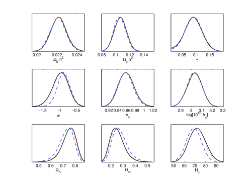
Figure 8: Marginalized parameter distributions in three models with free $w$. The solid black lines correspond to a model with $\alpha_{vis}=0$ and $c^{2}_{lam}=1$. The dotted red lines show the results from a model where $\alpha_{vis}$ is allowed to vary freely between $-20$ and $20$ and $c^{2}_{lam}=1$. The dashed blue lines show the constraints from a model with $\alpha_{vis}=0$ and $c_{lam}=0$.

5 Constraints from future data

As we have seen, only weak constraints can be found on the $c^{2}_{vis}$, $\alpha_{vis}$ and $c^{2}_{lam}$ parameters using present data. We have also argued that the effect of including other types of data sets, like LSS and SNIa, would not be very helpful, as such kinds of data sets are not affected significantly by these parameters. Also, unless $w$ is significantly below -1, they will not serve to break parameter degeneracies for the parameters studied here. Will it then be possible to improve our constraints with future CMB data?

To answer this question we have simulated a “perfect” CMB temperature data set, where the error bars are defined only from cosmic variance (CV) around a power spectrum generated from the best-fit $\Lambda$CDM model (with $w=-1$, $c^{2}_{vis}=0$ and $c^{2}_{lam}=1$) from WMAP data. The likelihood part of CosmoMC has been modified to use this perfect data instead of the WMAP measurements. The likelihood is calculated as in (Verde et al., 2003):

$$-2\log\mathcal{L}(x_{i};p_{i})=\sum_{\ell}(2\ell+1)\left[\ln\left(\frac{C_{\ell}^{model}}{C_{\ell}^{sim}}\right)+\frac{C_{\ell}^{sim}}{C_{\ell}^{model}}-1\right]$$ (7)

For this mock data set we have used multipoles from $l=2$ to $l=2000$ in our analysis, and also here we have added the same prior on $H_{0}$ and age as earlier. A completely noise-free data set is of course not realistic. However, it is an interesting case to study, since effects that cannot be seen here, will never be possible to see using a real CMB temperature experiment. Note that, when using this mock data set, we do not include any polarization data in our analysis.

In Figure 9 we show the constraints in the $\alpha_{vis}$-$w$ plane in a model with $c^{2}_{lam}=1$ and $\alpha_{vis}<0$. This is compared with the results from using WMAP data alone, as also shown in Figure 4. As we can see, even in this idealized case, we do not see any major improvement in our constraints on $\alpha_{vis}$. In this case the lower limit increases from $\alpha_{vis}>-0.23$ (from WMAP data) to $\alpha_{vis}>-0.22$.

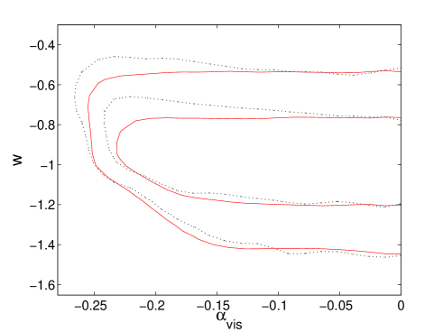
Figure 9: 68% and 95% contours of $\alpha_{vis}$ and $w$ in a model with $c^{2}_{lam}=1$ and using only ”perfect” CV limited CMB temperature data (solid lines). The dotted lines shows the results obtained when using WMAP3 data, as shown in Figure 4.

In Figure 10 we have used the CV limited mock data to redo one the most interesting case from the analysis with WMAP data, namely the constraints in the $c^{2}_{vis}$-$w$ plane with $w<-1$ and $c^{2}_{vis}<0$, as shown in Figure 3. We see that the constraints in this area improve slightly, but not very significantly. Using the CV-limited mock data we find $c^{2}_{vis}>-17.5$, compared to $c^{2}_{vis}>19.5$ using WMAP data.

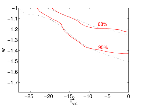
Figure 10: 68% and 95% contours of $c^{2}_{vis}$ and $w$ in a model with $c^{2}_{lam}=1$ and using only CV limited CMB temperature data (solid red lines). The dotted lines shows the results obtained when using WMAP3 data, as shown in Figure 3.

We have also redone the constraints on the dark energy sound speed, $c^{2}_{lam}$, using the “perfect” data set. In Figure 11 we show the confidence contours in the $c^{2}_{lam}$-$w$ and $c^{2}_{lam}$-$\Omega_{m}$ planes, as done earlier with WMAP data. In Figure 12 we have the corresponding 1-dimensional probability distribution. As we can see, using the perfect CMB temperature data, does not improve our constraints on this parameter at all.

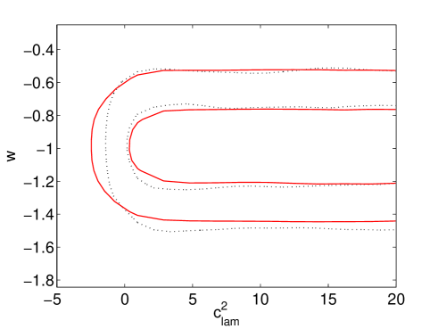
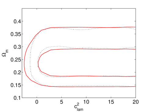
Figure 11: 68% and 95% confidence contours in the $c^{2}_{lam}$-$w$ and $c^{2}_{lam}$-$\Omega_{m}$ planes using only CV limited CMB temperature data (solid red lines). The black, dotted contours are the results obtained from using WMAP data, as shown in Figure 6. The constraints are not improved when using “perfect” data. In this model $\alpha_{vis}=0$.

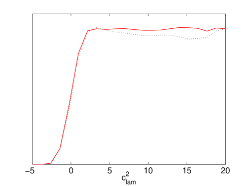
Figure 12: The marginalized probability distribution for $c^{2}_{lam}$ using only CV limited CMB temperature data (solid red line). The black, dotted line indicates the result from using WMAP data. The constraints are not improved by using “perfect” data. In this model $\alpha_{vis}=0$ and $w$ is allowed to vary freely.

That improved CMB data does not help to constrain dark matter properties, is not very surprising. As seen in Figures 1 and 2, effects occur mainly on large scales, where the error bars in the WMAP data already are dominated by cosmic variance.

6 Discussion and conclusions

We have investigated the possibility of using cosmological observations to constrain a possible dark energy anisotropic stress. We have parameterized the dark energy component in a very general way. Such generalized cosmological fluid is characterized by an equation of state ($w$), a speed of sound ($c^{2}_{lam}$) and an anisotropic stress ($\alpha_{vis}$ and $c^{2}_{vis}$). We have subjected this parameterization to the most detailed and most extensive scrutiny this far.

We have found that it is difficult to constrain the properties of an imperfect dark energy fluid. If the Universe resides in the phantom regime, with $w<-1$, one can put a weak lower limit on $c^{2}_{vis}$. In this case we found $c^{2}_{vis}>-19.5$ at 95% CL. However, $c^{2}_{vis}$ is not bounded from above. We also found that in a model with negative $\alpha_{vis}$, this parameter can be constrained to $\alpha_{vis}>-0.23$ at 95% CL using WMAP data. We found no upper limit on $\alpha_{vis}$ in models with $\alpha_{vis}>0$. These results reflect the fact that a dark energy fluid with nonzero $\alpha_{vis}$ generates shear stress which tends to smoothen its distribution. However, the consequences to phantom dark energy are qualitatively different and for such a fluid, with $w<-1$, a shear stress drives the clustering.

A similar conclusion applies to the dark energy sound speed, $c^{2}_{lam}$, where one also can put some lower limits, but no upper limits on its value.

Considering a simulated “perfect” CMB data set, only limited by cosmic variance, we found that improved CMB data sets are not likely to improve these constraints any further in the future.

These results stem from the fact that there is always an area in the parameter space describing the possible properties of dark energy, where the fluid is different from the cosmological constant or quintessence, but observationally indistinguishable. Optimistically though, our Universe could happen to reside in some other area of this parameter space. Indeed, in some special cases, one might be able to find a detect a possible imperfectness of the dark energy fluid.

One could consider dark matter and dark energy into a single imperfect fluid (Koivisto & Mota, 2006). Since then the effects of shear viscosity are present already in the earlier evolution of universe, they in general have observable consequences. This is somewhat related to models featuring the presence of early dark energy (Doran & Robbers, 2006) (which is excluded by our single-parameter description of the evolution of the dark energy equation of state). It could be therefore interesting to study how the previous constraints derived on the presence of early dark energy will be modified when one takes into account possible imperfect properties of the fluid.

The anisotropic stress of dark energy can have clear signatures in the case that it does not average exactly to zero at large scales. Then the nonzero $\sigma$ does not only appear as a statistically isotropic perturbation of the fluid, but will drive the overall expansion of the universe anisotropically. Clearly the resulting modifications of the Friedmann equation can be tightly constrained (Koivisto & Mota, 2007a).

However, such specific cases aside, the arguably simplest dark energy extension of the $\Lambda$CDM model introduces an equation of state $w\neq 1$. Inevitably, the more general model then generates dark energy perturbations, thus forcing one to specify also the two parameters $c^{2}_{lam}$ and $c^{2}_{vis}$. Again, arguably the simplest parameterization then considers these parameters constant in time. We have found then that a nonzero $\sigma$, which is expected for any realistic fluid, typically escapes detection in this three-parameter model. It seems that it is enough to know $w$, and that $c^{2}_{lam}$ and $\alpha_{vis}$ do not matter as long as they are positive.

The cosmological implication is that a canonical scalar field or perfect fluid representation might ultimately turn out to be a phenomenologically sufficient description of all the observational consequences of dark energy. The fundamental lesson is however that even then one cannot exclude, by appealing to observational evidence alone, the possibility of imperfectness in dark energy.

References

- Amendola (2000) Amendola L., 2000, Phys. Rev., D62, 043511
- Amendola et al. (2004) Amendola L., Kunz M., Sapone D., 2004, arXiv:0704.2421 [astro-ph]
- Armendariz-Picon (2004) Armendariz-Picon C., 2004, JCAP, 0407, 007
- Armendariz-Picon et al. (2001) Armendariz-Picon C., Mukhanov V. F., Steinhardt P. J., 2001, Phys. Rev., D63, 103510
- Astier et al. (2006) Astier P., et al., 2006, Astron. Astrophys., 447, 31
- Bagla et al. (2003) Bagla J. S., Jassal H. K., Padmanabhan T., 2003, Phys. Rev., D67, 063504
- Barrow (1997) Barrow J. D., 1997, Phys. Rev., D55, 7451
- Bean & Dore (2004) Bean R., Dore O., 2004, Phys. Rev., D69, 083503
- Bento et al. (2002) Bento M. C., Bertolami O., Sen A. A., 2002, Phys. Rev., D66, 043507
- Brevik et al. (2004) Brevik I., Nojiri S., Odintsov S. D., Vanzo L., 2004, Phys. Rev., D70, 043520
- Brookfield et al. (2006) Brookfield A. W., van de Bruck C., Mota D. F., Tocchini-Valentini D., 2006, Phys. Rev. Lett., 96, 061301
- Caldwell et al. (2003) Caldwell R., Cooray A., Melchiorri A., 2003, astro-ph/0703375
- Copeland et al. (2006) Copeland E. J., Sami M., Tsujikawa S., 2006, Int. J. Mod. Phys., D15, 1753
- Doran & Robbers (2006) Doran M., Robbers G., 2006, JCAP, 0606, 026
- Freedman et al. (2001) Freedman W. L., et al., 2001, Astrophys. J., 553, 47
- Gibbons (2002) Gibbons G. W., 2002, Phys. Lett., B537, 1
- Hinshaw et al. (2007) Hinshaw G., et al., 2007, Astrophys. J., 170, 288
- Hu (1998) Hu W., 1998, Astrophys. J., 506, 485
- Hu & Eisenstein (1999) Hu W., Eisenstein D. J., 1999, Phys. Rev., D59, 083509
- Ichiki & Takahashi (2007) Ichiki K., Takahashi T., 2007, astro-ph/0703549
- Kiselev (2004) Kiselev V. V., 2004, Class. Quant. Grav., 21, 3323
- Koivisto (2005) Koivisto T., 2005, Phys. Rev., D72, 043516
- Koivisto & Mota (2006) Koivisto T., Mota D. F., 2006, Phys. Rev., D73, 083502
- Koivisto & Mota (2007a) —, 2007a, arXiv:0707.0279 [astro-ph]
- Koivisto & Mota (2007b) —, 2007b, Phys. Lett., B644, 104
- Koivisto & Mota (2007c) —, 2007c, Phys. Rev., D75, 023518
- Lewis & Bridle (2002) Lewis A., Bridle S., 2002, Phys. Rev., D66, 103511
- Ma & Bertschinger (1995) Ma C.-P., Bertschinger E., 1995, Astrophys. J., 455, 7
- Mota & Shaw (2006) Mota D. F., Shaw D. J., 2006, Phys. Rev. Lett., 97, 151102
- Mota & Shaw (2007) —, 2007, Phys. Rev., D75, 063501
- Mota & van de Bruck (2004) Mota D. F., van de Bruck C., 2004, Astron. Astrophys., 421, 71
- Nojiri & Odintsov (2005) Nojiri S., Odintsov S. D., 2005, Phys. Rev., D72, 023003
- Page et al. (2007) Page L., et al., 2007, Astrophys. J., 170, 335
- Schimd et al. (2006) Schimd C., et al., 2006, astro-ph/0603158
- Tegmark et al. (2006) Tegmark M., et al., 2006, Phys. Rev., D74, 123507
- Verde et al. (2003) Verde L., Peiris H. V., Spergel D. N., Nolta M., Bennett C. L., Halpern M., Hinshaw G., Jarosik N., Kogut A., Limon M., Meyer S. S., Page L., Tucker G. S., Wollack E., Wright E. L., 2003, The Astrophysical Journal, 148, 195
- Weller & Lewis (2003) Weller J., Lewis A. M., 2003, Mon. Not. Roy. Astron. Soc., 346, 987
- Wetterich (1988) Wetterich C., 1988, Nucl. Phys., B302, 668
- Xia et al. (2007) Xia J.-Q., Cai Y.-F., Qiu T.-T., Zhao G.-B., Zhang X., 2007, astro-ph/0703202
- Zimdahl et al. (2001) Zimdahl W., Schwarz D. J., Balakin A. B., Pavon D., 2001, Phys. Rev., D64, 063501