Anisotropic fluxes and nonlocal interactions in MHD turbulence

Abstract

We investigate the locality or nonlocality of the energy transfer and of the spectral interactions involved in the cascade for decaying magnetohydrodynamic (MHD) flows in the presence of a uniform magnetic field $\bf B$ at various intensities. The results are based on a detailed analysis of three-dimensional numerical flows at moderate Reynold numbers. The energy transfer functions, as well as the global and partial fluxes, are examined by means of different geometrical wavenumber shells. On the one hand, the transfer functions of the two conserved Elsässer energies $E^{+}$ and $E^{-}$ are found local in both the directions parallel ($k_{\|}$-direction) and perpendicular ($k_{\perp}$-direction) to the magnetic guide-field, whatever the ${\bf B}$-strength. On the other hand, from the flux analysis, the interactions between the two counterpropagating Elsässer waves become nonlocal. Indeed, as the ${\bf B}$-intensity is increased, local interactions are strongly decreased and the interactions with small $k_{\|}$ modes dominate the cascade. Most of the energy flux in the $k_{\perp}$-direction is due to modes in the plane at $k_{\|}=0$, while the weaker cascade in the $k_{\|}$-direction is due to the modes with $k_{\|}=1$. The stronger magnetized flows tends thus to get closer to the weak turbulence limit where the three-wave resonant interactions are dominating. Hence, the transition from the strong to the weak turbulence regime occurs by reducing the number of effective modes in the energy cascade.

I Introduction

The existence of magnetic fields is known in many astrophysical objects such as interstellar medium, galaxies, accretion discs, star and planet interiors, or solar wind (see e.g. Zeldovich, Ruzmaikin & Sokoloff (1990)). In most of these systems, the magnetic fields are strong enough to play a significant dynamical role. The involved kinetic and magnetic Reynolds numbers in these astrophysical bodies are large enough so that the flows exhibit a turbulent behavior with a large continuous range of excited scales, from the largest where energy is injected towards the finest where energy is dissipated. In many cases, a strong large-scale magnetic field is present and induces dynamic anisotropy. Direct numerical simulations that examine in detail the turbulent processes in geo- and astrophysical plasmas are very difficult to achieve, for only rather modest Reynolds numbers can be reached with nowadays computers. One way around this difficulty is to model the small spatial and temporal scales to reproduce the large-scale behavior of turbulent flows. A more basic understanding of turbulence is thus needed to adequately model the flows, in particular when a uniform magnetic field, constant both in space and time, is applied.

As a first approximation, the incompressible magnetohydrodynamic (MHD) equations can be used to describe the evolution of both velocity, ${\bf u}$, and magnetic field, ${\bf b}$, fluctuations. In the presence of an uniform magnetic field ${\bf B}$ (magnetic fields are here expressed in velocity units), the Elsässer formulation of the MHD equations, with constant unit mass density, reads

$$\partial_{t}{\bf z}^{\pm}=\pm{\bf B}\cdot\nabla{\bf z}^{\pm}-{\bf z}^{\mp}\cdot\nabla{\bf z}^{\pm}-\nabla P+\nu\nabla^{2}{\bf z}^{\pm}$$ (1)

together with $\nabla\cdot{\bf z}^{\pm}=0$, where ${\bf z}^{\pm}={\bf u\pm b}$ are the Elsässer fluctuations, and $P$ is the total (kinetic plus magnetic) pressure. We assume here equal molecular viscosity $\nu$ and magnetic diffusivity $\eta$, in other words a unit magnetic Prandtl number ($P_{r}=\nu/\eta=1$). Hereafter, the direction along the ${\bf B}$ magnetic field is referred to as the parallel direction and the projection of the wavevectors along this direction is denoted $k_{\|}$, while the two directions of planes perpendicular to ${\bf B}$ are referred to as perpendicular directions, the wavevector projection onto such planes being denoted ${\bf k}_{\perp}$ with norm $k_{\perp}\equiv|{\bf k}_{\perp}|$.

For periodic boundary conditions, equations (1) have two independent invariants in the absence of molecular viscosity and magnetic diffusivity, namely the Elsässer energies :

$$E^{\pm}=\frac{1}{2}\int{{\bf z}^{\pm}}^{2}({\bf x})\ dx^{3}.$$ (2)

However, when very small viscosity and magnetic diffusivity are present, it is expected that the nonlinear terms cascade the energies between scales, in the so-called inertial range, up to smallest ones where dissipation becomes effective and removes energy from the system. The rate at which large scales lose energy is then controlled by the nonlinear terms ${\bf z}^{\mp}\cdot\nabla{\bf z}^{\pm}-\nabla P$ that are responsible for coupling different scales and cascading the energy towards smaller and smaller scales. The nature of the interactions among various scales in turbulent flows that lead to this cascade is a long standing problem. Understanding the involved mechanisms is very important to predict evolution of the large-scale flow behavior, and to estimate global quantities in astrophysical systems, such as the transport of angular momentum, and accretion rates in accretion discs.

High-Reynolds-number hydrodynamic turbulence, often investigated in the framework of statistically homogeneous and isotropic turbulence (which can be questionable in natural flows), is described to first order by the Kolmogorov theory Kolmogorov (1941). In this phenomenological description, interactions between eddies of similar size give the dominant contribution to the energy cascade. This assumption leads to an energy spectrum in $k^{-5/3}$ and an energy cascade rate proportional to $u_{rms}^{3}/L$, where $u_{rms}$ is the root-mean-square of the velocity at large scale and $L$ is the typical (large) flow scale.

The cascade in MHD turbulence is more complex, especially in the presence of a background magnetic field. Even in the simplest case of zero or small intensity of the ${\bf B}$-field, so that isotropy could be recovered, whether the MHD energy cascade can be described by a phenomenology à la Kolmogorov is still an open question. In particular, the assumption that interactions between similar size eddies (local interactions) are responsible for the cascade of energy to smaller scales has been questioned in turbulent MHD flows both by theoretical arguments Vermarev04 ; Verma, Ayyer, & Chandra (2005); Yousef, Rincon & Schekochihin (2007) and the use of numerical simulations Alexakis, Mininni & Pouquet (2005); Mininni, Alexakis & Pouquet (2005); Carati, et al. (2006). It has been shown for mechanically forced MHD turbulence there is a strong nonlocal coupling between the forced scales and the small scales of the inertial range. Moreover, the large-scale magnetic field generated by the dynamo action can also locally affect the small scales by suppressing the cascade rate in the same manner that an initially imposed uniform magnetic field would. In the other limit, a strong ${\bf B}$-field can lead to the flow bi-dimensionnalization, with a drastic reduction of the nonlinear transfers along the uniform magnetic field. For a ${\bf B}$-intensity (denoted $B$) well above the rms level of kinetic and magnetic fluctuations, the MHD turbulence may be dominated by the Alfvén waves dynamics, leading to wave (or weak) turbulence where the energy transfer, stemming from three-wave resonant interactions, can only increase perpendicular components of the wavevectors, i.e. components in planes perpendicular to the ${\bf B}$-direction ($k_{\perp}$-direction), the nonlinear transfers along ${\bf B}$ ($k_{\|}$-direction) being completely inhibited Galtier et al. (2000, 2002). How MHD turbulence moves from the weak turbulence limit, $B\gg u_{rms}$, to the strong turbulence limit, $B\sim u_{rms}$ and $B\sim 0$ (where isotropy could be recovered), is an open question.

Various authors have tried to give a physical description of the strong turbulence regime with $B\sim u_{rms}$. Iroshnikov Iroshnikov (1963) and Kraichnan Kraichnan (1965) first proposed a phenomenological description that takes into account the effect of a large-scale magnetic field by reducing the rate of the cascade due to the short time duration of individual collisions of $z^{\pm}$ wave packets. The resulting 1-D energy spectrum is then given by $E(k)\sim(\epsilon B)^{1/3}k^{-3/2}$. However, this description assumes isotropy and, while the effect of the large-scale field is taken into account by reducing the effective amplitude of the interactions, the interactions themselves are considered to be local. In order to take into account anisotropy in strong turbulence, a scale dependent anisotropy has been proposed (Goldreich & Sridhar, 1995), the turbulent $z^{\pm}_{l}$-eddies being such that the associated Alfvén $\tau_{{}_{A}}\sim l_{\|}/B$ and nonlinear $\tau_{{}_{NL}}\sim l_{\perp}/z$ times are equal (the so called critical balance), where $l_{\|}$ and $l_{\perp}$ are the typical length scales respectively parallel and perpendicular to the mean magnetic field. Repeating the Kolmogorov arguments, one ends up with a $E(k_{\|},k_{\perp})\sim k_{\perp}^{-5/3}$ energy spectrum with $k_{\|}\sim k_{\perp}^{2/3}$. Recently, this result has been generalized in an attempt to model MHD turbulence both in the weak and the strong limit, the ratio of the two time scales $\tau_{{}_{A}}/\tau_{{}_{NL}}$ being kept fixed but not necessarily of order one Galtier et al. (2005). In an other approach to obtain the transition from the strong to the weak turbulence limit (Matthaeus & Zhou, 1989; Zhou, Matthaeus & Dmitruk, 2004) suggested time scale for the energy cascade is given by the inverse average between the Alfvén and the nonlinear time scale $\tau^{-1}=\tau_{{}_{A}}^{-1}+\tau_{{}_{NL}}^{-1}$. All these models however assume locality of interactions that are also in question in anisotropic MHD turbulence Bhattacharjee & Ng (2001). A nonlocal model for anisotropic turbulence has been recently proposed by one of the authors Alexakis (2007); it assumes that the energy cascade is due to interactions between eddies with different parallel sizes and similar perpendicular scales, while a non-universal behavior is expected for moderate Reynold numbers.

Although very useful in getting a first order understanding of the processes involved in a turbulent cascade, cascade-energy models have to be unavoidably based on assumptions that need to be tested. To this respect, numerical simulations of the MHD equations are very valuable because they provide information about the evolution of the fields in the whole space, something not easily obtained from observations. Many numerical investigations have been performed during the last two decades (Mason, Cattaneo & Boldyrev, ; Müller & Grappin, 2005; Ng, Bhattacharjee, & Germaschewski, 2003; Dmitruk, Gomez, & Matthaeus, 2003; Maron & Goldreich, 2001; Cho & Vishniac, 2000; Biskamp & Müller, 2000; Ng & Bhattacharjee, 1996; Oughton, Priest, & Mattaheus, 1994) and, at the achieved Reynolds numbers, they have demonstrated that different power-law exponents are obtained depending on the chosen forcing. In this work, we use the results of numerical simulations of free decaying MHD flows at moderate Reynolds number to investigate the MHD interactions for various intensities of the external magnetic field. In particular, we try to investigate whether the transfer of energy in the parallel and perpendicular direction is local (i.e. the two energies $E^{\pm}$ cascade between nearby wavenumbers) or nonlocal (i.e. distant wavenumbers are involved in the cascade), and whether the coupling between the two oppositely moving waves ${\bf z}^{+}$ and ${\bf z}^{-}$ (that do not exchange energy) is local or not; and if not, which modes are responsible for the energy cascade.

The paper is organized as follows. In the next section, we give the precise definitions of the transfer functions and partial fluxes used to analyze the nature of the energy cascade. The details of the numerical simulations are given in Section IIIa. In Section IIIb, we investigate the locality or nonlocality of the energy transfers, and in section IIIc, we examine the nature of the interactions between the two ${\bf z}^{+}$ and ${\bf z}^{-}$ fields. We conclude and discuss our results in Section IV.

II Definitions

Our goal is to investigate the interactions among different scales. To define the notion of “scale”, we use the field Fourier transforms :

$${\bf\widehat{z}^{\pm}(k)}=\frac{1}{({2\pi})^{3}}\int{\bf{z^{\pm}}(x)}e^{-i{\bf k\cdot x}}dx^{3}$$ (3)

defined in a $2\pi$-periodic cube, such as

$${\bf z^{\pm}(x)}=\sum_{\bf k}{\bf\widehat{z}^{\pm}}({\bf k})e^{i{\bf k\cdot x}},$$ (4)

Similar size eddies will be considered as the ones whose Fourier transform contains similar wavenumbers.

In any basic flow interaction, three wavevectors are involved. For example, the evolution of a given Fourier amplitude $\widehat{\bf z}^{+}({\bf k})$ will be coupled to a $\widehat{\bf z}^{-}({\bf p})$ one and cascade the energy to the mode $\widehat{\bf z}^{+}({\bf q})$ such that the wavevectors satisfy ${\bf k+p+q}=0$. Note that the mode $\widehat{\bf z}^{-}({\bf p})$ does not gain or lose energy from this interaction since the two energies $E^{+}$ and $E^{-}$ are separately conserved. To obtain the cascade mean rate, one needs to average over all possible triadic interactions. To get a phenomenological understanding of the processes at play in MHD turbulence, we need to know if : i) most of the energetic exchanges occur between wavenumbers such that $|{\bf k}|\sim|{\bf q}|$ and ii) the energy flux is a result of spectral interactions of the two fields ${\bf z}^{\pm}$ with similar wavenumbers or not ($|{\bf k}|\sim|{\bf p}|$).

To address these questions, let us consider a partition of the wavevectors into non-overlapping sets $S^{\pm}_{{}_{K}}$ such that $S^{\pm}=\bigcup_{K=1}^{\infty}S^{\pm}_{{}_{K}}=\mathbb{Z}^{3}$. For example $S^{\pm}_{{}_{K}}$ could be the spherical shells of unit width and radius $K$, i.e. set of wavevectors k that have $K<|{\bf k}|\leq K+1$. We now define the filtered fields ${\bf z}^{\pm}_{{}_{K}}({\bf x})$ so that only modes in the set $S^{\pm}_{{}_{K}}$ are kept:

$${\bf z^{\pm}_{{}_{K}}(x)}=\sum_{{\bf k}\in S^{\pm}_{{}_{K}}}{\bf\widehat{z}^{\pm}}({\bf k})e^{i{\bf k\cdot x}}.$$ (5)

Clearly, one gets

$${\bf z^{\pm}(x)=\sum_{K}z^{\pm}_{{}_{K}}(x)}.$$ (6)

The triadic interactions among the different sets, say $S^{\pm}_{{}_{K}}$,$S^{\mp}_{{}_{P}}$ and $S^{\pm}_{{}_{Q}}$, are given by:

$$\mathcal{T}^{\pm}_{3}(K,P,Q)=-{\int{\bf z^{\pm}_{{}_{K}}}{\bf z^{\mp}_{{}_{P}}}\cdot\nabla{\bf z^{\pm}_{{}_{Q}}}dx^{3}}$$ (7)

that express the rates at which $E^{\pm}$ energies are transfered from $S^{\pm}_{{}_{Q}}$ to $S^{\pm}_{{}_{K}}$ sets due to the interactions with the modes belonging to $S^{\mp}_{{}_{P}}$ set. Note that the collection of sets $S^{+}$ and $S^{-}$ need not to be necessarily the same; for example, $S^{+}$ could be a collection of cylindrical shells while $S^{-}$ could be a collection of plane sheets. Adding over the index $P$ (all sets in $S^{\mp}$), we obtain the transfer functions :

$$\mathcal{T}^{\pm}(K,Q)=\sum_{P}\mathcal{T}^{\pm}_{3}(K,P,Q)=-{\int{\bf z^{\pm}_{{}_{K}}}{\bf z^{\mp}}\cdot\nabla{\bf z^{\pm}_{{}_{Q}}}dx^{3}}$$ (8)

that give the $E^{+}$ and $E^{-}$ transfer rates from $S^{\pm}_{{}_{Q}}$ to $S^{\pm}_{{}_{K}}$ sets due to all possible interactions. Note that the ${\bf z}^{+}$ field is not exchanging energy with the ${\bf z}^{-}$ field, and vice versa, but their interaction is responsible for the redistribution of the energy among various sets. $\mathcal{T}^{\pm}(K,Q)$ can give us information about the locality or nonlocality of the energy transfer, i.e. whether the energy is exchanged by nearby sets or long-range transfers from the large scales directly to the small scales are also involved.

However, the $\mathcal{T}^{\pm}(K,Q)$ transfer functions do not give us direct information on the scales of the two fields ${\bf z}^{+}$ and ${\bf z}^{-}$ that interact and contribute to the energy cascade. To investigate the locality on nonlocality of the interactions between the two Elsässer counterpropagating waves, we introduce the partial fluxes (see Alexakis (2005); Mininni, Alexakis & Pouquet (2005)) defined as:

$$\Pi^{\pm}_{{}_{P}}(K)= \sum_{K^{\prime}=0}^{K}\sum_{Q=0}^{\infty}\mathcal{T}^{\pm}_{3}(K^{\prime},P,Q)$$

$$= -\sum_{K^{\prime}=0}^{K}\int{\bf z^{\pm}_{{}_{K^{\prime}}}{\bf z}_{{}_{P}}^{\mp}\cdot\nabla{\bf z}^{\pm}}dx^{3}$$ (9)

that express the flux of energy out of the outer surface of the $S^{\pm}_{{}_{K}}$ shell due to the interactions with the $S^{\mp}_{P}$ shell. Summation over the whole $S^{\mp}$ collection of sets enable to recover the usual definition for the global fluxes :

$$\Pi^{\pm}(K)= \sum_{K^{\prime}=0}^{K}\sum_{Q=0}^{\infty}\sum_{P=0}^{\infty}\mathcal{T}^{\pm}_{3}(K^{\prime},P,Q)$$

$$= -\sum_{K^{\prime}=0}^{K}\int{\bf z^{\pm}_{{}_{K^{\prime}}}{\bf z}^{\mp}\cdot\nabla{\bf z}^{\pm}}dx^{3}$$ (10)

In the current work, we are going to use three different types of wavevector collections. We first consider spherical shells traditionally used in studies of isotropic turbulence so that a set $S_{{}_{K}}$ contains the wavevectors $\bf k$ such that $K\leq{|\bf k|}<K+1$. The second collection of sets are cylindrical shells along the direction of the guiding magnetic field. In this case, the set $S_{{}_{K}}$ contains the wavevectors $\bf k$ such that $K\leq k_{\perp}<K+1$ (with $k_{\perp}=\sqrt{k_{x}^{2}+k_{y}^{2}}$). Finally, we consider planes perpendicular to the ${\bf B}$-direction, so that the set $S_{{}_{K}}$ contains the wavevectors $\bf k$ whose $k_{\|}$-component satisfies $K\leq|k_{\|}|<K+1$ (where $k_{\|}$ stands for $k_{z}$).

III Numerical results

III.1 Numerical setup and initial conditions

We integrate numerically the three-dimensional incompressible MHD equations (1), in a $2\pi$-periodic box using a pseudo-spectral method with $256^{3}$ collocation points. The time marching uses an Adams-Bashforth Cranck-Nicholson scheme, i.e. a second-order finite-difference scheme. The initial kinetic and magnetic fields correspond to spectra proportional to $k^{2}exp(-k/2)^{2}$ for $k=[1,8]$, which means a flat modal spectrum for wavevector ${\bf k}$ up to $k=2$, to prevent any favored wavevector at time $t=0$, and the associated kinetic and magnetic energies are chosen equal, namely $E_{v}(t=0)=E_{b}(t=0)=1/2$, as in previous numerical studies (see Milano et al. (2001) and references therein). Moreover, the correlation between the velocity and magnetic field fluctuations, as measured by the cross-correlation coefficient defined by $2\int{\bf v}({\bf x})\cdot{\bf b}({\bf x)}\ dx^{3}/(E_{v}+E_{b})$, is initially less than $1\%$. At scale injection, the initial kinetic and magnetic Reynolds numbers are about $800$ for flows at $\nu=\eta\sim 4\times 10^{-3}$, with $u_{rms}=b_{rms}=1$ and an isotropic integral scale $L=2\pi\int{k^{-1}E_{v}(k)dk}/\int{E_{v}(k)dk}$ of about $\pi$. The dynamics of the flow is then let to freely evolve. The parametric study according to the intensity of the background magnetic field ${\bf B}$ is performed for four different values : $B=0,1,5$ and $15$. All the simulations are run up to a computational time $t_{max}=15$, at which the loss of the total energy (kinetic plus magnetic) is about $95\%$ for the simulation with $B=0$, $90\%$ for $B=1$, and $83\%$ for the $B=5$ and $B=15$ runs.

Figure 1 shows the time evolution of the total energy, $E(t)=(E^{+}(t)+E^{-}(t))/2$, and the total enstrophy, $\Omega(t)=1/2\int[{{\bf w}}^{2}({\bf x},t)+{{\bf j}}^{2}({\bf x},t)]\ dx^{3}$ (where ${\bf w}=\nabla\times{\bf u}$ stands for the vorticity field, and ${\bf j}=\nabla\times{\bf b}$ for the current), for the four different simulations. One can note that the influence of the strength of the external magnetic field clearly slows down the flow dynamics. Note that the $B=5$ and $B=15$ flows present a very similar temporal behavior in energy as well as in enstrophy.

Figure 1: Temporal evolutions of the total energy (top panel) and of the total enstrophy (bottom panel) for the four examined intensities of the ${\bf B}$ applied field.

The analysis that follows in the next subsection is based on the outputs of the runs at $t=4$ where the spectra are fully developed and all runs wave roughly the same enstrophy. At this time, the cross-correlation coefficient, that one can also write $(E^{+}-E^{-})/(E^{+}+E^{-})$, is about $3.6\%$ and $2.5\%$ respectively for the $B=0$ and $B=1$ flows, while it is close to $1.6\%$ for $B=5$ and $1\%$ for $B=15$, with thus a lesser increase in the stronger magnetized flows. The energy spectra in the perpendicular direction to the uniform ${\bf B}$-field $E(k_{\perp})=1/2\int[\hat{\bf z}^{-}(k)]^{2}+[\hat{\bf z}^{+}(k)]^{2}k_{\perp}dk_{\|}$ and in the parallel one $E(k_{\|})=1/2\int[\hat{\bf z}^{-}(k)]^{2}+[\hat{\bf z}^{+}(k)]^{2}k_{\perp}dk_{\perp}$ are shown in Figure 2 at the same time. Clearly as the magnetic field intensity is increased, the spectrum in the $k_{\|}$-direction becomes steeper. Because the planes at $k_{\|}=0$ and $k_{\|}=1$ are shown to play an important role in the cascade, we mention here their properties in more details. In absence of the applied magnetic field, the modes with $k_{\|}=0$ contain $32\%$ of the total energy and $8\%$ of the total enstrophy, and the $k_{\|}=1$ modes have $30\%$ of the total energy and $10\%$ of the total enstrophy. In the strongly anisotropic case, $B=15$, the $k_{\|}=0$ modes contain $55\%$ of the total energy and $34\%$ of the total enstrophy while the $k_{\|}=1$ modes have $37\%$ of the total energy and $35\%$ of the total enstrophy.

Figure 2: Total energy spectra in the perpendicular (top panel) and the parallel (bottom) directions.

In our investigation, we focus on the cascade of the $E^{-}$ energy. The $E^{+}$ cascade has also been analyzed and it gives qualitatively similar results. We consider separately the cascades in the perpendicular and parallel directions relatively to the applied magnetic field. For this reason, we examine three different types of flux; (i) the flux across spheres of radius $k\equiv|{\bf k}|$ that corresponds to an isotropic analysis, (ii) the flux across cylinders of radius $k\equiv k_{\perp}$ that corresponds to the flux in the perpendicular direction and (iii) the flux across planes located at $k\equiv|k_{\|}|$ that corresponds to the flux in the direction parallel to the ${\bf B}$-field direction. Figure 3 shows these three fluxes, as a function of $k$, for various ${\bf B}$-intensities. It is clear that as the amplitude of the large-scale magnetic field is increased, the parallel flux is strongly reduced. For $B=5$, this flux is reduced by more than one order of magnitude when compared to the case with $B=0$. For $B=15$, the parallel flux across planes is very small and it even takes negative values.

Figure 3: Fluxes $\Pi_{S}^{-}(k)$ across : (i) spheres (solid line), (ii) cylinders (dashed line), (iii) planes (doted line), for $B=0$ (top panel), $B=1$ (mid panel) and $B=5$ (bottom panel).

III.2 Energy transfers

We now examine the locality or nonlocality of energy transfers from our numerical data. For two different values of the uniform magnetic field, namely $B=0$ and $B=5$, Figure 4 shows a shadow-graph of the transfer function $\mathcal{T}^{-}(K,Q)$ between ${\bf z^{-}_{K}}$ and ${\bf z^{-}_{Q}}$, defined in Eqs. (5) and (8), for energy exchanges across cylindrical shells (perpendicular cascade), while Figure 5 shows the transfer function $\mathcal{T}^{-}(K,Q)$ for energy exchanges across plane sheets (parallel cascade). In all cases, the transfer is concentrated along the diagonal $K=Q$ line. This indicates that the cascade happens through a local energy exchange. Similar results are obtained from the two other simulations at $B=1$ and $B=15$ (not shown). Note the highly non-linear color bar used for the parallel cascade in the $B=5$ case. This choice is due to the extremely fast decrease of the amplitude of $\mathcal{T}^{-}(K,Q)$ as the wavenumbers $K$ and $Q$ become large.

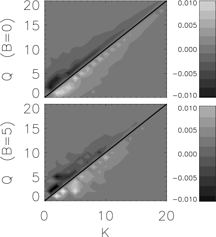
Figure 4: The transfer function $\mathcal{T}^{-}(K,Q)$ that demonstrates the energy exchange between cylindrical shells of radius $K$ and $Q$. Solid lines show the diagonal $K=Q$. The top panel shows the $B=0$ case and the bottom panel the $B=5$ case.

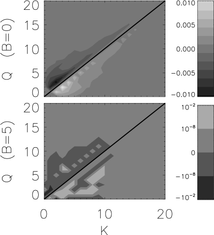
Figure 5: The transfer function $\mathcal{T}^{-}(K,Q)$ that demonstrates energy exchanges between plane sheets located at distance $K$ and $Q$ from origin, for $B=0$ (top panel) and $B=5$ (bottom panel) cases. Solid lines indicate the $K=Q$ diagonal.

From Figures 4 and 5, it can be seen that most of the energy exchange happens close to the diagonal line ($K=Q$). This implies that waves traveling in the same direction exchange energy between similar size wavenumbers. In the strong $B$ flow, some inverse cascade is also visible in the parallel cascade (Fig. 5) as indicated by the dark lines below the diagonal and the bright ones above the diagonal.

To get a better understanding of the $\mathcal{T}^{\pm}(K,Q)$ transfer functions, we look at a single wavenumber $Q$. Figure 6 displays $\mathcal{T}^{-}(K,Q)$ for the perpendicular cascade (cylinders) at $Q=10$ as a function of $K$, whereas Figure 7 shows it for the parallel cascade (planes) at $Q=10$. To compare the results obtained from the different $B$ cases, the $\mathcal{T}^{-}(K,Q)$ amplitudes are normalized so that all transfers are of the same order of magnitude. Positive values of $\mathcal{T}^{-}(K,Q)$ imply that the shell $K$ receives energy from the shell $Q=10$ (Fig. 6, perpendicular case) and (Fig. 7, parallel case) while negative values of $\mathcal{T}^{-}(K,Q)$ mean that the shell $K$ gives energy to the shell $Q=10$.

Figure 6: The energy transfer function $\mathcal{T}^{-}(K,Q)$ for the perpendicular cascade (cylinders) for $Q=10$ as a function of $K$, from the runs with $B=0$ (solid line), $B=1$ (dashed line) and $B=5$ (dotted line). Amplitudes of $\mathcal{T}^{-}(K,Q)$ are normalized to have the same order of magnitude than in the $B=0$ case.

Figure 7: The energy transfer function $\mathcal{T}^{-}(K,Q)$ for the parallel cascade (planes) for $Q=10$ as a function of $K$, from the data at $B=0$ (solid line), $B=1$ (dashed line) and $B=5$ (dotted line). Amplitudes of $\mathcal{T}^{-}(K,Q)$ are normalized to have the same order of magnitude than in the $B=0$ case.

For the perpendicular cascade, the shell $Q=10$ receives most energy from slightly smaller wavenumbers than $K=10$ and it gives energy to slightly larger wavenumbers. This implies a locality in the energy transfer, since it is mostly the nearby cylindrical shells that exchange energy. The parallel cascade presents a similar behavior; the shell $Q=10$ receives energy from slightly smaller wavenumbers than $K=10$ and it gives energy to slightly larger wavenumbers. Note however that for the $B=5$ flow, there is also some trace of an inverse cascade (energy transfer from the wavenumber $Q=10$ to the wavenumber $K=8$). This local behavior has also been found in isotropic ($B=0$) decaying MHD turbulence simulations Debliquy, Verma & Carati (2005). Nevertheless, we need to note that in forced MHD turbulence where the magnetic field is generated by dynamo action, strong nonlocal transfers also exist Alexakis, Mininni & Pouquet (2005); Carati, et al. (2006). Whether these nonlocal transfers are present in the forced anisotropic regime still needs further studies.

III.3 Nonlinear interactions between ${\bf z}^{+}$ and ${\bf z}^{-}$

The analysis of the energy transfer functions has thus shown that the energy cascades locally. As a result, each Elsässer field, ${\bf z}^{+}$ or ${\bf z}^{-}$, exchanges energy between waves traveling in the same direction of similar size. Nonetheless, this does not mean that interactions among oppositely traveling waves are local. In the limit of very large intensities of the background magnetic field, where the weak turbulence theory is valid, the energy cascade is due to interactions with the modes in the plane at $k_{\|}=0$. Therefore, modes with $k_{\|}\geq 1$ interact with modes $k_{\|}\ll 1$ to cascade the energy. To that respect, the interactions are nonlocal since short waves (large $k_{\|}$) interact with long waves (small $k_{\|}$ ) to cascade the energy. To investigate how close to the weak turbulence regime we are, we plot in Figure 8 the total energy flux $\Pi^{-}(K)$, defined in Eq. (10), across cylinders together with the partial flux $\Pi_{P=0}^{-}(K)$, defined in Eq. (9) due to interactions with just $k_{\|}=0$ modes.

Figure 8: The total energy flux $\Pi^{-}(K)$ (solid line) across cylinders of radius $K$ together with the partial flux $\Pi_{P=0}^{-}(K)$ (dashed line) for the four different values of $B$, from $B=0$ (top panel) up to $B=15$ (bottom panel).

As the strength of the uniform magnetic field is increased, the flux due to the interactions with the $k_{\|}=0$ modes become more and more dominant. In the $B=15$ flow, the global and partial fluxes across cylinders become almost indistinguishable suggesting that interactions with the modes in the plane at $k_{\|}=0$ are responsible for the energy cascade. This means that the flow dynamics tends to be closer to a weak turbulence regime where the three-wave resonant interactions are dominating.

A different behavior is obtained for the parallel energy cascade. When a mode $\widehat{\bf z}^{-}({\bf k})$ interacts with a mode $\widehat{\bf z}^{+}({\bf p})$, the $\widehat{\bf z}^{-}({\bf k})$ energy will move to the wavevector $\bf q$ so that the relation $\bf k+p+q=0$ holds. If however $\bf p$ belongs to the wavevector set with $p_{\|}=0$, this relation then reads $k_{\|}+q_{\|}=0$ in the parallel direction, i.e. $|k_{\|}|=|q_{\|}|$. Therefore, the energy remains in spectral planes located at the same distance from the origin. As a result, interactions with the $k_{\|}=0$ modes cannot contribute to the energy cascade in the parallel direction. In this case, the closest modes to the $k_{\|}=0$ modes are the ones that gives most of the energy flux. Figure 9 shows the total energy flux across planes and the partial flux only due to interactions with the modes in the plane at $k_{\|}=1$ (the closest to the $k_{\|}=0$ plane). As the amplitude of the ${\bf B}$-field is increased, most of the parallel flux comes from modes with $k_{\|}=1$. Here, we need to note that the flux in the parallel direction is much noisier than the flux in the perpendicular direction and that it often presents negative values (absolute values are plotted in the bottom panel of Fig. 9). A thorough analysis of the parallel cascade would require to average many data outputs which is not possible in the case of a freely decaying flows. Such an analysis is left for future work.

Figure 9: The total energy flux $\Pi^{-}(K)$ (solid line) across planes at $k_{\|}=K$ together with the partial flux $\Pi_{P=1}^{-}(K)$ (dashed line) for the four different values of $B$ from $B=0$ (top panel) up to $B=15$ (bottom panel).

IV Conclusion and Discussion

In this work we examine the energy cascade and the interactions between different scales for freely decaying MHD flows in the presence of a uniform magnetic field. Our analysis is based on data obtained from direct numerical simulations of the MHD equations with four different intensities of the applied magnetic field, in an attempt to study the transition from strong to weak turbulence limit. One clearly established result is that, as the strength of the uniform magnetic field is increased, the energy spectrum becomes anisotropic with most of the energy concentrated in the small $k_{\|}$ wavenumbers, as already known Oughton, Priest, & Mattaheus (1994). It is further shown that the energy flux in the parallel direction (relatively to the uniform magnetic field) is also strongly suppressed when the guiding field in introduced.

To investigate the locality or nonlocality of the spectral interactions, we measure the transfer functions for the parallel and the perpendicular cascade. The transfer functions in the parallel and perpendicular directions are found local whatever the strength of the external magnetic field. As a result, the coupling between modes that travel in the same direction is local and the energy exchange occurs between similar size eddies. This behavior has been shown to hold in decaying isotropic MHD turbulence simulations (with $B=0$) Debliquy, Verma & Carati (2005). However, in the presence of a mechanical forcing, strong nonlocal interactions have been observed with a direct energy transfer from the forced scale to the inertial range scales Alexakis, Mininni & Pouquet (2005); Carati, et al. (2006). If this nonlocal behavior persists in the anisotropic case still needs further investigations.

The locality or nonlocality of the interactions between oppositely moving waves ($z^{+}$ and $z^{-}$), that do not exchange energy, is measured by means of partial fluxes in the parallel and the perpendicular directions due to the coupling in different spectral planes. This coupling between oppositely propagating modes does not appear local. As the amplitude of the applied magnetic field is increased, most of the interactions occur with the $k_{\|}=0$ modes that are dominant in cascading the energy. Most of the energy flux is thus in the perpendicular direction, since the $k_{\|}=0$ modes do not contribute to the energy cascade in the parallel direction. Hence, the stronger magnetized flows tends to present a dynamics close to the weak turbulence limit where the three-wave resonant interactions are responsible for the cascade process. This also partly explains the similar temporal evolution in the $B=5$ and $B=15$ regimes (see Figure 1) since, in both cases, most of the cascade is due to the $k_{\|}=0$ modes.

For the parallel cascade, the interactions are slightly different. As already said, this is due to the inability of the $k_{\|}=0$ modes to cascade the energy in the parallel direction. In that case, the modes with the smallest but not zero $k_{\|}$ ($k_{\|}\simeq 1$) are the ones responsible for the cascade. This behavior is in qualitative agreement with the description of a recent phenomenological model Alexakis (2007). However, the lack of resolution does not allow to pursue a quantitative comparison.

Finally, we would like to emphasize that we analyze here numerical data of freely decaying MHD flows submitted to an external magnetic field whose amplitude is varied, while all the other parameters are kept unchanged (periodic boundary conditions, unit magnetic Prandtl number, initial conditions and Reynolds number). Thus, one should be cautious in any attempt to generalize the obtained results, e.g. forced turbulence could lead to different behaviors and should be studied separately. The results could also be dependent on the kinetic Reynolds number as well on the magnetic Prandtl number. Furthermore the use of a refined spectral grid in the parallel direction, allowing the presence of more modes with $k_{\|}\simeq 0$, could alter the energy cascade.