Statistics of quantum transmission in one dimension with broad disorder

Abstract

We study the statistics of quantum transmission through a one-dimensional disordered system modelled by a sequence of independent scattering units. Each unit is characterized by its length and by its action, which is proportional to the logarithm of the transmission probability through this unit. Unit actions and lengths are independent random variables, with a common distribution that is either narrow or broad. This investigation is motivated by results on disordered systems with non-stationary random potentials whose fluctuations grow with distance.

In the statistical ensemble at fixed total sample length four phases can be distinguished, according to the values of the indices characterizing the distribution of the unit actions and lengths. The sample action, which is proportional to the logarithm of the conductance across the sample, is found to obey a fluctuating scaling law, and therefore to be non-self-averaging, in three of the four phases. According to the values of the two above mentioned indices, the sample action may typically grow less rapidly than linearly with the sample length (underlocalization), more rapidly than linearly (superlocalization), or linearly but with non-trivial sample-to-sample fluctuations (fluctuating localization).

,

1 Introduction

The phenomenon of localization of a quantum particle by a random potential is well understood (see, e.g., [1, 2]), especially in the one-dimensional case (see, e.g., [3]). It is known that this phenomenon has a major influence on coherent quantum transport. The amplitude ${\cal T}$ of transmission through a sample is therefore a quantity of central importance in this context. The interpretation of experiments about the effects of localization on transport is done with the help of the (two-probe) Landauer formula [4, 5], which relates the probability of transmission $|{{\cal T}}|^{2}$ through a sample to its conductance $g$ at zero temperature,

$$g=\displaystyle{\displaystyle 2e^{2}\over\displaystyle h}\,|{{\cal T}}|^{2}.$$ (1.1)

In the one-dimensional disordered systems usually considered, namely those modelled by stationary random potentials with short-range correlations, all the eigenstates are exponentially localized. Thus any sample whose length $L$ is much greater than the localization length $\xi$ is an insulator [1, 2, 3]. The probability of transmission is a strongly fluctuating quantity in the insulating regime and so it is preferable to consider its logarithm [6, 7]. It is therefore appropriate to introduce the sample action

$$S=-\displaystyle{\displaystyle 1\over\displaystyle 2}\ln|{{\cal T}}|^{2}.$$ (1.2)

The statistics of the transmission probability in the insulating regime are determined by the distribution of $S$. The average of the sample action over all the configurations of the random potential grows asymptotically as

$$\langle S\rangle\approx\displaystyle{\displaystyle L\over\displaystyle\xi}.$$ (1.3)

The sample action $S$ is self-averaging in the strong sense that each cumulant of its distribution increases in direct proportion to the sample length [3]. Said otherwise, the distribution of $S$ is similar to that of the free energy of a one-dimensional disordered thermodynamical system; the transfer matrix formalism [3, 8, 9] is well adapted to demonstrate this deep analogy.

The situation is quite different for one-dimensional disordered systems modelled by non-stationary random potentials whose fluctuations grow with distance [10, 11, 12]. Typical eigenstates turn out to be superlocalized rather than localized in samples whose length exceeds a well-defined crossover length $\ell_{\rm cr}$, which diverges in the weak-disorder regime. The action $S$ for long enough samples ($L\gg\ell_{\rm cr}$) exhibits two novel features with respect to the usual one-dimensional localization problem: it grows faster than linearly with $L$ and it is not self-averaging in the sense that it keeps on fluctuating in arbitrarily large samples. For instance, in the case of a self-affine Gaussian random potential whose fluctuations increase as a power law with a Hurst exponent $H$ in the range $0<H<1$, the scaling law of the sample action is the following [12]:

$$S\approx\left(\displaystyle{\displaystyle E\over\displaystyle\ell_{\rm cr}^{H}}\right)^{1/2}L^{1+H/2}\,\cal Y.$$ (1.4)

Here $E$ denotes the energy of the particle, $\ell_{\rm cr}$ the above mentioned crossover length, and $\cal Y$ a rescaled random variable whose distribution is a universal function in the sense that it is determined by one parameter only, namely the value of $H$.

In this work we address the question whether the properties of the two previous classes of models can be combined into a single model of one-dimensional disordered system, in which the concomitant features of self-averaging and conventional localization hold in a certain range of parameters but are replaced by the concomitant properties of lack of self-averaging and departure from conventional localization in another range. More specifically, the purpose of this paper is to present and study a model which exhibits the above properties and is simple enough to be exactly solvable by analytical means. The article is organized as follows. In Section 2 we describe the model and set the notation used throughout the paper. In Section 3 we study the statistics of the transmission probability through samples consisting of a large but fixed number $N$ of units. In Section 4 we study the statistics of the transmission probability through samples whose length $L$ is large but fixed. The results and their physical consequences are discussed in Section 5. Finally, an appendix is devoted to the derivation of the formula of the sample action on which our calculations are based.

2 The model

The model considered in this paper consists of a disordered array of elementary units, put together end to end on a line. Each of these units consists of a disordered part connected to two perfect leads, as shown pictorially in Figure 1 where disordered segments are represented by boxes, leads by line segments, and the connection between each unit and the next one by a dot.

Figure 1: Schematic picture of the model considered in this paper, consisting of a disordered array of elementary units whose lengths $\ell_{n}$ and actions $s_{n}$ are independent random variables.

The $n$th unit has a length $\ell_{n}$ and its transport properties are characterized by the transmission and reflection amplitudes $t_{n}$, $r_{n}$, and $r^{\prime}_{n}$. We shall work in the regime in which the probability of transmission through every unit is very small ($|{t_{n}}|^{2}\ll 1$). As explained in the appendix, in this weak transmission regime and with the simplifying assumption that the reflection phases are random and uniform, the law of addition for the actions (A.24) holds.

The basic observables of our model are therefore the following. For a sample made of $N$ units, we consider its total action $S_{N}$ and total length $L_{N}$. These quantities are simply expressed as sums,

$$S_{N}=\sum_{n=1}^{N}s_{n},\quad L_{N}=\sum_{n=1}^{N}\ell_{n},$$ (2.1)

where the actions $s_{n}$ and lengths $\ell_{n}$ of the units are the microscopic variables of the model. The simplicity of these definitions of the basic observables makes the present model exactly solvable by analytical means.

Disorder is introduced into the model by assuming that the unit actions $s_{n}$ and the unit lengths $\ell_{n}$ are mutually independent random variables. The actions $s_{n}$ are assumed to be greater than some minimal action $s_{\rm min}>0$ and to be distributed identically, with a common continuous probability distribution defined by the density $f_{s}(s)$. Similarly, the lengths $\ell_{n}$ are assumed to be greater than some minimal length $\ell_{\rm min}>0$ and to be distributed identically, with a common distribution defined by the density $f_{\ell}(\ell)$. Thus the sequences of random variables $S_{N}$ and $L_{N}$ obtained by adding units to a sample constitute examples of a renewal process (see, e.g., [13]).

The samples may be classified in two different ways, either by their number $N$ of units, ignoring their length, or by their length $L$, ignoring the number of units they consist of. These two different points of view give rise to the following two different statistical ensembles.

• Statistical ensemble of the samples with a fixed number $N$ of units. In this ensemble the sample action $S_{N}$ and the sample length $L_{N}$, equation (2.1), are the sums of a fixed number $N$ of independent random variables.

• Statistical ensemble of the samples with a fixed length $L$. In this ensemble the sample action, denoted by $S_{L}$, is the sum of a $\it random$ number $N_{L}$ of independent random variables,

  $$S_{L}=\sum_{n=1}^{N_{L}}s_{n}.$$ (2.2)

  For a given configuration $\{\ell_{n}\}$ of the unit lengths, $N_{L}$ is defined as the number of units which are entirely contained in the sample of fixed length $L$. This choice is motivated by simplicity. The random number $N_{L}$ therefore obeys the inequalities

  $$L_{N_{L}}<L<L_{N_{L}+1},\quad\hbox{i.e.,\ \ }\sum_{n=1}^{N_{L}}\ell_{n}<L<\sum_{n=1}^{N_{L}+1}\ell_{n}.$$ (2.3)

  Since the length of any unit is greater than the minimal length $\ell_{\rm min}$, the random integer $N_{L}$ can take any value between 0 and its maximal value $[L/\ell_{\rm min}]$, the symbol $[x]$ denoting the integer part of the number $x$.

These two statistical ensembles will be carefully distinguished throughout the following and successively investigated in Sections 3 and 4. The statistics of the transmission may indeed exhibit qualitative differences between both ensembles.

Generalizing a notation already introduced, we shall denote the probability density of a random variable $\eta$ by $f_{\eta}(\eta)$. The moment generating function and moment function of $\eta$ will be denoted by $\widehat{f}_{\eta}(x)$ and $m_{\eta}(p)$ respectively. These functions are defined as

$$\widehat{f}_{\eta}(x)=\langle{\rm e}^{-x\eta}\rangle=\int{\rm e}^{-x\eta}\,f_{\eta}(\eta)\,{\rm d}\eta,\quad m_{\eta}(p)=\langle\eta^{p}\rangle=\int\eta^{p}\,f_{\eta}(\eta)\,{\rm d}\eta,$$ (2.4)

where the real parts of the complex variables $x$ and $p$ take their values in ranges such that the integrals are convergent. The moment function is only defined for a positive random variable $\eta$. The inverse formulae are

$$f_{\eta}(\eta)=\int\displaystyle{\displaystyle{\rm d}x\over\displaystyle 2\pi{\rm i}}\,{\rm e}^{x\eta}\,\widehat{f}_{\eta}(x)=\int\displaystyle{\displaystyle{\rm d}p\over\displaystyle 2\pi{\rm i}}\,\eta^{-p-1}\,m_{\eta}(p).$$ (2.5)

The moment generating function and the moment function are linked together by the identity

$$m_{\eta}(-p)=\displaystyle{\displaystyle 1\over\displaystyle\Gamma(p)}\int_{0}^{\infty}\widehat{f}_{\eta}(x)\,x^{p-1}\,{\rm d}x\quad(\mathop{{\rm Re}}p>0),$$ (2.6)

where the symbol $\mathop{{\rm Re}}z$ denotes the real part of the complex number $z$ and $\Gamma(z)$ the gamma function. The identity (2.6) is easily verified by using the definition of $\widehat{f}_{\eta}(x)$, equation (2.4), on the right-hand side and evaluating the integral in $x$ with the help of the first of the pair of identities ([14, p. 317])

$$\matrix{\displaystyle\int_{0}^{\infty}x^{p-1}\,{\rm e}^{-xy}\,{\rm d}x=\displaystyle{\displaystyle\Gamma(p)\over\displaystyle y^{p}}\quad\hfill&(\mathop{{\rm Re}}p>0,~{}\mathop{{\rm Re}}y>0),\hfill\cr\displaystyle\mathrel{\mathop{\int}\limits_{\mathop{{\rm Re}}y>0}}\displaystyle{\displaystyle{\rm d}y\over\displaystyle 2\pi{\rm i}}\,\displaystyle{\displaystyle{\rm e}^{xy}\over\displaystyle y^{p}}=\displaystyle{\displaystyle x^{p-1}\over\displaystyle\Gamma(p)}\hfill&(\mathop{{\rm Re}}x>0).\hfill}$$ (2.7)

It is convenient to characterize the probability densities $f_{s}(s)$ and $f_{\ell}(\ell)$ by the exponents $\mu$, $\nu$ and the scales $s_{0}$, $\ell_{0}$ of the power law fall off of the corresponding complementary distribution functions:

$$\matrix{\mathop{{\rm Prob}}\left\{s_{1}>s\right\}=\displaystyle\int_{s}^{\infty}f_{s}(s_{1})\,{\rm d}s_{1}\approx\left(\displaystyle{\displaystyle s_{0}\over\displaystyle s}\right)^{\mu}\quad\hfill&(s\to\infty),\cr\mathop{{\rm Prob}}\left\{\ell_{1}>\ell\right\}=\displaystyle\int_{\ell}^{\infty}f_{\ell}(\ell_{1})\,{\rm d}\ell_{1}\approx\left(\displaystyle{\displaystyle\ell_{0}\over\displaystyle\ell}\right)^{\nu}\quad\hfill&(\ell\to\infty).}$$ (2.8)

The notation $x\approx y$ used here means that the ratio $x/y$ tends to unity in the considered limit; it will be used extensively in the following. We shall also use the notation $x\sim y$, which has the weaker meaning that $x$ and $y$ are only proportional in the considered limit, up to an unimportant prefactor.

We shall consider the following classes of probability distributions $f_{s}(s)$ and $f_{\ell}(\ell)$.

• Narrow distributions ($\mu>2$; $\nu>2$). These are the distributions whose first two moments at least are finite. Thus we have

  $$\matrix{\widehat{f}_{s}(x)=1-x\langle s\rangle+{\textstyle{\frac{1}{2}}}x^{2}\langle s^{2}\rangle+\cdots,\hfill\cr\widehat{f}_{\ell}(x)=1-x\langle\ell\rangle+{\textstyle{\frac{1}{2}}}x^{2}\langle\ell^{2}\rangle+\cdots,\hfill}$$ (2.9)

  where $\langle s\rangle$ and $\langle s^{2}\rangle$ (resp. $\langle\ell\rangle$ and $\langle\ell^{2}\rangle$) are the first two moments of $f_{s}(s)$ (resp. $f_{\ell}(\ell)$). Said otherwise, the narrow distributions are those for which the central limit theorem holds.

  The narrow distributions with a complementary distribution function that falls off more rapidly than any power law (we have then formally $\mu=\infty$ or $\nu=\infty$) have the property that all their moments are finite, and so

  $$\matrix{\widehat{f}_{s}(x)=\displaystyle\sum_{k\geq 0}\displaystyle{\displaystyle(-x)^{k}\over\displaystyle k!}\langle s^{k}\rangle=\exp\left(\sum_{k\geq 1}\displaystyle{\displaystyle(-x)^{k}\over\displaystyle k!}\langle\!\langle s^{k}\rangle\!\rangle\right),\hfill\cr\widehat{f}_{\ell}(x)=\displaystyle\sum_{k\geq 0}\displaystyle{\displaystyle(-x)^{k}\over\displaystyle k!}\langle\ell^{k}\rangle=\exp\left(\sum_{k\geq 1}\displaystyle{\displaystyle(-x)^{k}\over\displaystyle k!}\langle\!\langle\ell^{k}\rangle\!\rangle\right),\hfill}$$ (2.10)

  where $\langle s^{k}\rangle$ and $\langle\!\langle s^{k}\rangle\!\rangle$ (resp. $\langle\ell^{k}\rangle$ and $\langle\!\langle\ell^{k}\rangle\!\rangle$) are the moment and cumulant of order $k$ of $f_{s}(s)$ (resp. $f_{\ell}(\ell)$).

• Broad distributions ($\mu<2$; $\nu<2$). These are the distributions whose second moment is infinite. In other words, the broad distributions are those for which the central limit theorem does not hold. Two cases have to be distinguished. If $\mu<1$ (resp. $\nu<1$), the first moment of $f_{s}(s)$ (resp. $f_{\ell}(\ell)$) is also infinite. On the other hand, if $1<\mu<2$ (resp. $1<\nu<2$), the first moment of $f_{s}(s)$ (resp. $f_{\ell}(\ell)$) is still finite. The expansions of the moment generating functions as $x\to 0^{+}$ begin as

  $$\matrix{\widehat{f}_{s}(x)=\left\{\matrix{1-\Gamma(1-\mu)(s_{0}x)^{\mu}+\cdots\hfill&(\mu<1),\hfill\cr 1-\langle s\rangle x+|{\Gamma(1-\mu)}|(s_{0}x)^{\mu}+\cdots\hfill\quad&(1<\mu<2),\cr}\right.\cr\cr\widehat{f}_{\ell}(x)=\left\{\matrix{1-\Gamma(1-\nu)(\ell_{0}x)^{\nu}+\cdots\hfill&(\nu<1),\hfill\cr 1-\langle\ell\rangle x+|{\Gamma(1-\nu)}|(\ell_{0}x)^{\nu}+\cdots\hfill\quad&(1<\nu<2),\cr}\right.}$$ (2.11)

  where the dots represent regular and singular terms of higher order [15]. Disorder modelled by broad distributions will be called broad disorder.

3 Transmission statistics in the ensemble of samples with a fixed number $N$ of units

The statistics of the transmission probability through samples with a fixed number $N$ of units are determined by the distribution of the sample action $S_{N}$, equation (2.1). We shall be interested here in the scaling properties of $S_{N}$ in the large $N$ limit. This study may be considered as an introduction to that done in Section 4, in which the most interesting results are derived.

It is useful to introduce the moment generating function $\widehat{f}_{S_{N}}(x)$ of $S_{N}$. Since the unit actions are mutually independent random variables with a common distribution, $\widehat{f}_{S_{N}}(x)$ takes the form

$$\widehat{f}_{S_{N}}(x)=\widehat{f}_{s}(x)^{N}.$$ (3.1)

The scaling law of $S_{N}$ can be obtained from the expression of this quantity in the large $N$ and small $x$ limits. Three cases have to be distinguished, as the expansions (2.9) and (2.11) of $\widehat{f}_{s}(x)$ for small $x$ are different for $\mu>2$, $\mu<1$, and $1<\mu<2$. We shall discuss these three cases below in this order. The results of this section also apply to the distribution of the sample length $L_{N}$, provided we replace the index $\mu$ and the parameters $\langle s\rangle$ and $s_{0}$ in the obtained results by the index $\nu$ and the parameters $\langle\ell\rangle$ and $\ell_{0}$ respectively.

3.1 Self-averaging with normal fluctuations: $\mu>2$

This is the easiest case to study, as the distribution of the unit actions $s_{n}$ is narrow. Using the expression (2.9) of $\widehat{f}_{s}(x)$ in (3.1), we obtain

$$\widehat{f}_{S_{N}}(x)\approx\exp\left(N\left(-x\langle s\rangle+{\textstyle{\frac{1}{2}}}x^{2}\langle\!\langle s^{2}\rangle\!\rangle\right)\right)$$ (3.2)

in the relevant regime ($N$ large and $x$ small). Setting

$$S_{N}\approx N\langle s\rangle+(N\langle\!\langle s^{2}\rangle\!\rangle)^{1/2}\,\eta,$$ (3.3)

we find that the moment generating function of the rescaled random variable $\eta$ is

$$\widehat{f}_{\eta}(y)={\rm e}^{y^{2}/2}.$$ (3.4)

Equation (3.3) gives the scaling law of the sample action in the present case. The fluctuations of $S_{N}$ about its mean $N\langle s\rangle$ increase as $N^{1/2}$, and so become negligible in relative value in the large $N$ limit. Hence $S_{N}$ is self-averaging. The distribution of $\eta$ is Gaussian,

$$f_{\eta}(\eta)=\displaystyle{\displaystyle{\rm e}^{-\eta^{2}/2}\over\displaystyle\sqrt{2\pi}}.$$ (3.5)

In the case of narrow distributions with a complementary distribution function that falls off more rapidly than any power law, $S_{N}$ is self-averaging in the strong sense that each cumulant of its distribution is exactly proportional to $N$:

$$\langle\!\langle S_{N}^{k}\rangle\!\rangle=N\langle\!\langle s^{k}\rangle\!\rangle.$$ (3.6)

This can be checked by using the expression (2.10) of $\widehat{f}_{s}(x)$ in (3.1).

3.2 Fluctuating scaling law: $\mu<1$

In this case the distribution of the unit actions $s_{n}$ is broad, with an infinite mean $\langle s\rangle$. Using the first expression (2.11) of $\widehat{f}_{s}(x)$ in (3.1), we obtain

$$\widehat{f}_{S_{N}}(x)\approx\exp\left(-N\Gamma(1-\mu)(s_{0}x)^{\mu}\right)$$ (3.7)

in the relevant regime ($N$ large and $x$ small). Setting

$$S_{N}\approx s_{0}(\Gamma(1-\mu))^{1/\mu}N^{1/\mu}\,{\cal L}_{\mu},$$ (3.8)

we find that the positive rescaled random variable ${\cal L}_{\mu}$ has a non-trivial limiting distribution, whose moment generating function is

$$\widehat{f}_{{\cal L}_{\mu}}(y)={\rm e}^{-y^{\mu}}.$$ (3.9)

Equation (3.8) gives the scaling law of the sample action in the present case. It shows that $S_{N}$ increases as $N^{1/\mu}$, that is, faster than the number $N$ of units, because the exponent $1/\mu$ is greater than unity. Furthermore, $S_{N}$ is not self-averaging but keeps on fluctuating in the large $N$ limit. The result (3.8) therefore appears as a fluctuating scaling law. The expression of the distribution of the rescaled random variable ${\cal L}_{\mu}$ is obtained by using (3.9) in the first of the formulae (2.5),

$$f_{{\cal L}_{\mu}}({\cal L})=\mathrel{\mathop{\int}\limits_{\mathop{{\rm Re}}y>0}}\displaystyle{\displaystyle{\rm d}y\over\displaystyle 2\pi{\rm i}}\,{\rm e}^{y{\cal L}-y^{\mu}}.$$ (3.10)

This probability density is referred to as the (properly normalized) Lévy law of index $\mu$. It is a non-trivial universal function in the sense that it is determined by one parameter only, namely the value of $\mu$. References [16] provide a comprehensive presentation of Lévy laws, and References [17] provide overviews of applications of Lévy variables in Physics.

Expanding ${\rm e}^{-y^{\mu}}$ as a power series in the integrand of (3.10) and integrating term by term with the help of the second of the identities (2.7), we obtain the convergent expansion

$$f_{{\cal L}_{\mu}}({\cal L})=\sum_{k\geq 1}\displaystyle{\displaystyle(-1)^{k}\over\displaystyle k!\,\Gamma(-k\mu)}\,{\cal L}^{-(1+k\mu)}.$$ (3.11)

Using the complement formula for the gamma function, we find the alternative form

$$f_{{\cal L}_{\mu}}({\cal L})=\sum_{k\geq 1}\displaystyle{\displaystyle(-1)^{k-1}\over\displaystyle k!}\,\displaystyle{\displaystyle\sin(k\pi\mu)\over\displaystyle\pi}\,\Gamma(1+k\mu)\,{\cal L}^{-(1+k\mu)}.$$ (3.12)

The behaviour of the probability density $f_{{\cal L}_{\mu}}({\cal L})$ at large values of ${\cal L}$ is determined by the leading order term of this expansion,

$$f_{{\cal L}_{\mu}}({\cal L})\approx\displaystyle{\displaystyle\sin\pi\mu\over\displaystyle\pi}\,\Gamma(1+\mu)\,{\cal L}^{-(1+\mu)}\quad({\cal L}\to\infty).$$ (3.13)

Its behaviour at small values of ${\cal L}$ is obtained from (3.10) by means of the method of steepest descent. We thus find an exponentially fast fall off:

$$f_{{\cal L}_{\mu}}({\cal L})\sim\exp\left(-(1-\mu)\left(\displaystyle{\displaystyle\mu\over\displaystyle{\cal L}}\right)^{\mu/(1-\mu)}\right)\quad({\cal L}\to 0).$$ (3.14)

The density $f_{{\cal L}_{\mu}}({\cal L})$ admits a particularly simple expression in closed form for $\mu=1/2$, which is

$$f_{{\cal L}_{1/2}}({\cal L})=\displaystyle{\displaystyle{\rm e}^{-1/(4{\cal L})}\over\displaystyle 2\sqrt{\pi{\cal L}^{3}}}.$$ (3.15)

The expression of the moment function $m_{{\cal L}_{\mu}}(p)$ may be derived starting from (2.6). Using (3.9) in the right-hand side of the identity, we obtain it in three steps. We first evaluate the integral with the help of the relation ([14, p. 342])

$$\int_{0}^{\infty}x^{p-1}{\rm e}^{-x^{\mu}}\,{\rm d}x=\displaystyle{\displaystyle 1\over\displaystyle\mu}\Gamma(p/\mu)\quad(\mu>0,~{}\mathop{{\rm Re}}p>0).$$ (3.16)

We then rewrite the result using the difference formula for the gamma function. We finally extend the obtained result to negative values of $\mathop{{\rm Re}}p$ by analytic continuation. We thus find the simple formula

$$m_{{\cal L}_{\mu}}(p)=\displaystyle{\displaystyle\Gamma(1-p/\mu)\over\displaystyle\Gamma(1-p)}\quad(\mathop{{\rm Re}}p<\mu).$$ (3.17)

3.3 Self-averaging with anomalous fluctuations: $1<\mu<2$

In this case the distribution of the unit actions $s_{n}$ is still broad, but it has a finite mean $\langle s\rangle$. Using the second expression (2.11) of $\widehat{f}_{s}(x)$ in (3.1), we obtain

$$\widehat{f}_{S_{N}}(x)\approx\exp\Bigl{(}N\left(-\langle s\rangle x+|{\Gamma(1-\mu)}|\,(s_{0}x)^{\mu}\right)\Bigr{)}$$ (3.18)

in the relevant regime ($N$ large and $x$ small). Setting

$$S_{N}\approx N\langle s\rangle+s_{0}|{\Gamma(1-\mu)}|^{1/\mu}N^{1/\mu}\,{\cal L}_{\mu},$$ (3.19)

we find that the moment generating function of the rescaled random variable ${\cal L}_{\mu}$ is now

$$\widehat{f}_{{\cal L}_{\mu}}(y)={\rm e}^{y^{\mu}}.$$ (3.20)

Equation (3.19) gives the scaling law of the sample action in the present case. This expression involves two different microscopic characteristics of the distribution $f_{s}(s)$, namely the mean $\langle s\rangle$ and the amplitude $s_{0}$ of the power law tail (2.8). The fluctuations of $S_{N}$ about its mean $N\langle s\rangle$ increase as $N^{1/\mu}$, with $1/2<1/\mu<1$. On the one hand, these fluctuations are much smaller than the mean action in the large $N$ limit, and so $S_{N}$ is self-averaging. On the other hand, these fluctuations increase more rapidly than $N^{1/2}$, the power law of the central limit theorem involved in the expression (3.3). Furthermore, the distribution of the rescaled random variable ${\cal L}_{\mu}$ is not Gaussian.

Using (3.20), we obtain that ${\cal L}_{\mu}$ is distributed according to the following Lévy law of index $\mu$:

$$f_{{\cal L}_{\mu}}({\cal L})=\mathrel{\mathop{\int}\limits_{\mathop{{\rm Re}}y>0}}\displaystyle{\displaystyle{\rm d}y\over\displaystyle 2\pi{\rm i}}\,{\rm e}^{y{\cal L}+y^{\mu}}.$$ (3.21)

This probability density is universal, as it only depends on the value of the index $\mu$. It is non-vanishing for all values of ${\cal L}$. Its fall off at large positive values of ${\cal L}$ can be derived by linearizing (3.21) as

$$f_{{\cal L}_{\mu}}({\cal L})\approx\mathrel{\mathop{\int}\limits_{\mathop{{\rm Re}}y>0}}\displaystyle{\displaystyle{\rm d}y\over\displaystyle 2\pi{\rm i}}\,{\rm e}^{y{\cal L}}\,y^{\mu}.$$ (3.22)

Using again the second of the identities (2.7), we thus obtain

$$f_{{\cal L}_{\mu}}({\cal L})\approx\displaystyle{\displaystyle|{\sin\pi\mu}|\over\displaystyle\pi}\,\Gamma(1+\mu)\,{\cal L}^{-(1+\mu)}\quad({\cal L}\to+\infty).$$ (3.23)

This expression is the first term of an expansion analogous to (3.12). This expansion is, however, asymptotic but divergent in the present case. The behaviour of $f_{{\cal L}_{\mu}}({\cal L})$ at large negative values of ${\cal L}$ is obtained from (3.21) by means of the method of steepest descent. We thus find

$$f_{{\cal L}_{\mu}}({\cal L})\sim\exp\left(-(\mu-1)\left(\displaystyle{\displaystyle|{{\cal L}}|\over\displaystyle\mu}\right)^{\mu/(\mu-1)}\right)\quad({\cal L}\to-\infty).$$ (3.24)

Since the exponent $\mu/(\mu-1)$ is larger than 2, this fall off is of a superexponential type.

4 Transmission statistics in the ensemble of samples with a fixed length $L$

The statistics of the transmission probability through samples with a fixed length $L$ are determined by the distribution of the sample action $S_{L}$, equation (2.2). The random character of $S_{L}$ has two origins, as it is the sum of a random number $N_{L}$ of independent random variables. We shall be interested here in the scaling properties of $S_{L}$ in the limit of large values of $L$.

It is again useful to introduce the moment generating function of the sample action. Its expression is now

$$\widehat{f}_{S_{L}}(x,L)=\sum_{n\geq 0}p_{n}(L)\,\widehat{f}_{S_{n}}(x),$$ (4.1)

where $p_{n}(L)=\mathop{{\rm Prob}}\left\{N_{L}=n\right\}$ is the probability that a sample of length $L$ consists of exactly $n$ units and $\widehat{f}_{S_{n}}(x)$ the moment generating function corresponding to this particular number of units. Using (3.1), we obtain

$$\widehat{f}_{S_{L}}(x,L)=\sum_{n\geq 0}p_{n}(L)\,\widehat{f}_{s}(x)^{n}.$$ (4.2)

When dealing with functions $f(L)$ that depend on the sample length, it will prove useful to use their Laplace transform $\widetilde{f}(u)$ with respect to this variable,

$$\widetilde{f}(u)=\int_{0}^{\infty}{\rm e}^{-uL}\,f(L)\,{\rm d}L.$$ (4.3)

Equation (4.2) becomes

$$\widetilde{\widehat{f}_{S_{L}}}(x,u)=\sum_{n\geq 0}\widetilde{p}_{n}(u)\,\widehat{f}_{s}(x)^{n}.$$ (4.4)

The expression of the Laplace transform $\widetilde{p}_{n}(u)$ can be obtained as follows. The definition (2.3) of $N_{L}$ implies

$$p_{n}(L) = \mathop{{\rm Prob}}\left\{L_{n}<L<L_{n+1}\right\}$$ (4.5)

$$= \mathop{{\rm Prob}}\left\{L>L_{n}\right\}-\mathop{{\rm Prob}}\left\{L>L_{n+1}\right\}.$$

The Laplace transform of the first of these probabilities is simply

$$\int_{0}^{\infty}\mathop{{\rm Prob}}\left\{L>L_{n}\right\}\,{\rm e}^{-uL}\,{\rm d}L = \left\langle\int_{L_{n}}^{\infty}{\rm e}^{-uL}\,{\rm d}L\right\rangle$$ (4.6)

$$= \displaystyle{\displaystyle\langle{\rm e}^{-uL_{n}}\rangle\over\displaystyle u}=\displaystyle{\displaystyle\widehat{f}_{L_{n}}(u)\over\displaystyle u}=\displaystyle{\displaystyle\widehat{f}_{\ell}(u)^{n}\over\displaystyle u},$$

where the last equality has been obtained in analogy with the derivation of (3.1). The Laplace transform of the second probability is obtained upon replacing $n$ by $n+1$ in (4.6). It follows that (see, e.g., [15])

$$\widetilde{p}_{n}(u)=\widehat{f}_{\ell}(u)^{n}\,\displaystyle{\displaystyle 1-\widehat{f}_{\ell}(u)\over\displaystyle u}\qquad(n\geq 0).$$ (4.7)

Using (4.7) in (4.4), we find that the Laplace transform of the moment generating function has the following closed form expression:

$$\widetilde{\widehat{f}_{S_{L}}}(x,u)=\displaystyle{\displaystyle 1-\widehat{f}_{\ell}(u)\over\displaystyle u(1-\widehat{f}_{\ell}(u)\widehat{f}_{s}(x))}.$$ (4.8)

This equation is analogous to the Montroll-Weiss equation [18], which is well known in the theory of the continuous time random walks (see, e.g., [19]).

In the following, the scaling law of $S_{L}$ will be derived by using (4.8) in the small $x$ and small $u$ limits. The expressions (2.9) and (2.11) of $\widehat{f}_{s}(x)$ are different for $\mu>1$ and $\mu<1$, as well as those of $\widehat{f}_{\ell}(u)$ for $\nu>1$ and $\nu<1$. This leads to four different phases, which are identified by the conditions ($\mu>1$, $\nu>1$), ($\mu<1$, $\nu>1$), ($\mu>1$, $\nu<1$), and ($\mu<1$, $\nu<1$). We shall discuss these four phases in this order. For the sake of simplicity we shall not distinguish the situations of normal and anomalous fluctuations when the sums are self-averaging. Said otherwise, we shall not discuss separately the cases $\mu>2$ and $1<\mu<2$, nor the cases $\nu>2$ and $1<\nu<2$.

4.1 Phase I: $\mu>1$ and $\nu>1$

In this phase both means $\langle s\rangle$ and $\langle\ell\rangle$ are finite. The result (3.3) implies that $S_{N}\approx N\langle s\rangle$ and similarly that $L_{N}\approx N\langle\ell\rangle$, up to fluctuations that become negligible in relative value in the large $N$ limit. Eliminating $N$ between both estimates, we obtain

$$S_{L}\approx\displaystyle{\displaystyle\langle s\rangle\over\displaystyle\langle\ell\rangle}\,L,$$ (4.9)

again up to fluctuations that become negligible in relative value at large $L$. In order to obtain more accurate estimates of the mean $\langle S_{L}\rangle$ and the fluctuations about it, more restrictive conditions on the distributions $f_{\ell}$ and $f_{s}$ are needed.

Let us consider first the case of narrow distributions with $\mu>2$ and $\nu>2$. Using the expressions (2.9) of $\widehat{f}_{s}(x)$ and $\widehat{f}_{\ell}(u)$ in (4.8) and expanding this formula to second order in $x$ and $u$, we find that the mean and variance of the distribution of the sample action have the following expressions:

$$\langle S_{L}\rangle\approx\displaystyle{\displaystyle\langle s\rangle\over\displaystyle\langle\ell\rangle}\left(L+\displaystyle{\displaystyle\langle\!\langle\ell^{2}\rangle\!\rangle-\langle\ell\rangle^{2}\over\displaystyle 2\langle\ell\rangle}\right),$$ (4.10)

$$\langle\!\langle S_{L}^{2}\rangle\!\rangle\approx\displaystyle{\displaystyle\langle\ell\rangle^{2}\langle\!\langle s^{2}\rangle\!\rangle+\langle s\rangle^{2}\langle\!\langle\ell^{2}\rangle\!\rangle\over\displaystyle\langle\ell\rangle^{3}}L.$$ (4.11)

Equation (4.10) shows that the actual expression of the mean is not exactly the one given by (4.9). There is a finite correction term which is proportional to $\langle\!\langle\ell^{2}\rangle\!\rangle-\langle\ell\rangle^{2}=\langle\ell^{2}\rangle-2\langle\ell\rangle^{2}$ and so may be of either sign. Equation (4.11) indicates that the variance increases in direct proportion to $L$. The first correction to this leading order result, which has not been written explicitly, is a constant term for $\nu>3$ but grows as $\langle s\rangle^{2}L^{3-\nu}$ for $2<\nu<3$.

We also consider the case of narrow distributions with a complementary distribution function that falls off more rapidly than any power law. In this case $S_{L}$ is self-averaging in the strong sense that each cumulant of its distribution increases in direct proportion to $L$:

$$\langle\!\langle S_{L}^{k}\rangle\!\rangle\approx a_{k}L.$$ (4.12)

The expressions of the coefficients $a_{k}$ can be obtained as follows. Equation (4.12) means that the moment generating function $\widehat{f}_{S_{L}}(x,L)$ has the following exponential growth for large values of the sample length:

$$\widehat{f}_{S_{L}}(x,L)\sim{\rm e}^{A(x)L}.$$ (4.13)

Here $A(x)$ is the generating function of the coefficients $a_{k}$,

$$A(x)=\sum_{k\geq 1}\displaystyle{\displaystyle(-x)^{k}\over\displaystyle k!}\,a_{k}.$$ (4.14)

Equation (4.13) in turn implies that the Laplace transform $\widetilde{\widehat{f}_{S_{L}}}(x,u)$ has a simple pole of the form

$$\widetilde{\widehat{f}_{S_{L}}}(x,u)\sim\displaystyle{\displaystyle 1\over\displaystyle u-A(x)}.$$ (4.15)

On the other hand, (4.8) shows that $\widetilde{\widehat{f}_{S_{L}}}(x,u)$ has poles whenever $\widehat{f}_{\ell}(u)\widehat{f}_{s}(x)=1$. Hence the generating function $A(x)$ is determined by the implicit equation

$$\widehat{f}_{\ell}(A(x))\widehat{f}_{s}(x)=1.$$ (4.16)

Using the expression (2.10) of $\widehat{f}_{s}(x)$ and $\widehat{f}_{\ell}(x)$ in this equation and expanding it as a power series in $x$, we can derive the expressions of the coefficients $a_{k}$ in a recursive way. We find

$$\matrix{a_{1}=\displaystyle{\displaystyle\langle s\rangle\over\displaystyle\langle\ell\rangle},\hfill\cr a_{2}=\displaystyle{\displaystyle\langle\ell\rangle^{2}\langle\!\langle s^{2}\rangle\!\rangle+\langle s\rangle^{2}\langle\!\langle\ell^{2}\rangle\!\rangle\over\displaystyle\langle\ell\rangle^{3}},\hfill\cr a_{3}=\displaystyle{\displaystyle\langle\ell\rangle^{4}\langle\!\langle s^{3}\rangle\!\rangle-\langle\ell\rangle\langle s\rangle^{3}\langle\!\langle\ell^{3}\rangle\!\rangle+3\langle\ell\rangle^{2}\langle s\rangle\langle\!\langle\ell^{2}\rangle\!\rangle\langle\!\langle s^{2}\rangle\!\rangle+3\langle s\rangle^{3}\langle\!\langle\ell^{2}\rangle\!\rangle^{2}\over\displaystyle\langle\ell\rangle^{5}},}$$ (4.17)

and so on. As expected, the expression of the coefficient $a_{1}$ (resp. $a_{2}$) agrees with the one obtained from (4.10) (resp. (4.11)).

4.2 Phase II: $\mu<1$ and $\nu>1$

In this phase the mean $\langle\ell\rangle$ is finite, but the mean $\langle s\rangle$ is infinite. The fact that $\langle\ell\rangle$ is finite implies that the number of units increases as $N\approx L/\langle\ell\rangle$, by analogy with (3.3). We therefore surmise that the scaling law of $S_{L}$ is similar to the one of $S_{N}$ in the case $\mu<1$.

The scaling law of $S_{L}$ can be obtained as follows. Using the first expression (2.11) of $\widehat{f}_{s}(x)$ and the expression (2.9) of $\widehat{f}_{\ell}(u)$ in (4.8), we obtain

$$\widetilde{\widehat{f}_{S_{L}}}(x,u)\approx\left(u+\displaystyle{\displaystyle\Gamma(1-\mu)(s_{0}x)^{\mu}\over\displaystyle\langle\ell\rangle}\right)^{-1}$$ (4.18)

in the relevant regime ($x$ and $u$ small). The calculation of the inverse Laplace transform of $\widetilde{\widehat{f}_{S_{L}}}(x,u)$ gives

$$\widehat{f}_{S_{L}}(x,L)\approx\exp\left(-\Gamma(1-\mu)(s_{0}x)^{\mu}\displaystyle{\displaystyle L\over\displaystyle\langle\ell\rangle}\right).$$ (4.19)

We note that this expression becomes identical to (3.7) if we replace the ratio $L/\langle\ell\rangle$ by the number $N$ of units. This allows us to conclude that the scaling law of $S_{L}$ in Phase II is

$$S_{L}\approx s_{0}\left(\Gamma(1-\mu)\right)^{1/\mu}\left(\displaystyle{\displaystyle L\over\displaystyle\langle\ell\rangle}\right)^{1/\mu}\,{\cal L}_{\mu},$$ (4.20)

where the rescaled random variable ${\cal L}_{\mu}$ is distributed according to the Lévy law, equation (3.10). This result agrees with our surmise.

4.3 Phase III: $\mu>1$ and $\nu<1$

In this phase the mean $\langle s\rangle$ is finite but the mean $\langle\ell\rangle$ is infinite. The fact that $\langle s\rangle$ is finite implies that $S_{N}\approx N\langle s\rangle$, by virtue of (3.3). We therefore surmise that the fluctuations of $S_{L}$ are similar here to those of the number $N_{L}$ of units in the samples.

Following our surmise, we begin by deriving the scaling form of the expression of $p_{n}(L)$ in the limit of large values of $L$. Using the first expression (2.11) of $\widehat{f}_{\ell}(u)$ in (4.7), we obtain

$$\widetilde{p}_{n}(u)\approx\Gamma(1-\nu)\ell_{0}^{\nu}u^{\nu-1}\,\exp\Bigl{(}-\Gamma(1-\nu)(\ell_{0}u)^{\nu}n\Bigr{)}$$ (4.21)

in the relevant regime ($n$ large, $u$ small), and so

$$p_{n}(L)\approx\Gamma(1-\nu)\ell_{0}^{\nu}\mathrel{\mathop{\int}\limits_{\mathop{{\rm Re}}u>0}}\displaystyle{\displaystyle{\rm d}u\over\displaystyle 2\pi{\rm i}}\,u^{\nu-1}\,\exp\Bigl{(}-\Gamma(1-\nu)(\ell_{0}u)^{\nu}n+uL\Bigr{)}.$$ (4.22)

Let us introduce a rescaled variable $Z_{\nu}$ by setting

$$n\approx\displaystyle{\displaystyle 1\over\displaystyle\Gamma(1-\nu)}\left(\displaystyle{\displaystyle L\over\displaystyle\ell_{0}}\right)^{\nu}Z_{\nu}.$$ (4.23)

This positive random variable has a limiting distribution which is easily obtained from (4.22). Setting $z=uL$, we find

$$f_{Z_{\nu}}(Z)=\mathrel{\mathop{\int}\limits_{\mathop{{\rm Re}}z>0}}\displaystyle{\displaystyle{\rm d}z\over\displaystyle 2\pi{\rm i}}\,z^{\nu-1}\,{\rm e}^{z-Zz^{\nu}}.$$ (4.24)

This probability density admits an expression in closed form for $\nu=1/2$, case in which it is a half-Gaussian:

$$f_{Z_{1/2}}(Z)=\displaystyle{\displaystyle{\rm e}^{-Z^{2}/4}\over\displaystyle\sqrt{\pi}}\quad(Z>0).$$ (4.25)

The random variable $Z_{\nu}$ can be expressed as

$$Z_{\nu}={{\cal L}_{\nu}}^{-\nu},$$ (4.26)

where ${\cal L}_{\nu}$ is distributed according to the Lévy law, equation (3.10). Indeed, setting $Z={\cal L}^{-\nu}$ and $z=x{\cal L}$ in (4.24), we obtain the following expression for the probability density of ${\cal L}_{\nu}$:

$$f_{{\cal L}_{\nu}}({\cal L})=\displaystyle{\displaystyle\nu\over\displaystyle{\cal L}}\mathrel{\mathop{\int}\limits_{\mathop{{\rm Re}}x>0}}\displaystyle{\displaystyle{\rm d}x\over\displaystyle 2\pi{\rm i}}\,x^{\nu-1}\,{\rm e}^{x{\cal L}-x^{\nu}}.$$ (4.27)

This expression is then put into the canonical form (3.10) by means of an integration by parts.

The expression of the moment function of $Z_{\nu}$ is readily obtained by means of (3.17) and (4.26). We find

$$m_{Z_{\nu}}(p)=\displaystyle{\displaystyle\Gamma(1+p)\over\displaystyle\Gamma(1+p\nu)}\quad(\mathop{{\rm Re}}p>-1).$$ (4.28)

This result implies that the distribution of $Z_{\nu}$ is narrow in the strong sense that all its moments are finite. Setting $p=k$ in (4.28), we indeed obtain

$$\langle Z_{\nu}^{k}\rangle=\displaystyle{\displaystyle k!\over\displaystyle\Gamma(1+k\nu)}$$ (4.29)

for any integer $k$.

The relations (4.23) and (4.26) may also be found in the following heuristic way. By analogy with (3.8), the sample length $L_{N}$ has the following fluctuating scaling law in the case $\nu<1$:

$$L_{N}=\ell_{0}(\Gamma(1-\nu))^{1/\nu}\,N^{1/\nu}\,{\cal L}_{\nu}.$$ (4.30)

Expressing $N$ in this equation in terms of the other quantities, we obtain both above relations at once.

Let us now turn to the scaling law of $S_{L}$. Using the first expression (2.11) of $\widehat{f}_{\ell}(u)$ and the expression (2.9) of $\widehat{f}_{s}(x)$ in (4.8), we obtain

$$\widetilde{\widehat{f}_{S_{L}}}(x,u)\approx\displaystyle{\displaystyle\Gamma(1-\nu)\ell_{0}^{\nu}u^{\nu-1}\over\displaystyle x\langle s\rangle+\Gamma(1-\nu)(\ell_{0}u)^{\nu}}$$ (4.31)

in the relevant regime ($x$ and $u$ small), and so

$$\widetilde{f}_{S_{L}}(S_{L},u)\approx\displaystyle{\displaystyle\Gamma(1-\nu)\ell_{0}^{\nu}u^{\nu-1}\over\displaystyle\langle s\rangle}\,\exp\left(-\Gamma(1-\nu)(\ell_{0}u)^{\nu}\displaystyle{\displaystyle S_{L}\over\displaystyle\langle s\rangle}\right).$$ (4.32)

We note that this expression becomes identical to (4.21) if we replace the ratio $S_{L}/\langle s\rangle$ by the number $n$ of units. This allows us to conclude that the scaling law of $S_{L}$ in Phase III is

$$S_{L}\approx\displaystyle{\displaystyle\langle s\rangle\over\displaystyle\Gamma(1-\nu)}\left(\displaystyle{\displaystyle L\over\displaystyle\ell_{0}}\right)^{\nu}Z_{\nu}.$$ (4.33)

Our surmise has proved correct, as the same random variable $Z_{\nu}$, equation (4.26), enters the scaling laws of the number of units and of the sample action.

4.4 Phase IV: $\mu<1$ and $\nu<1$

This last phase is the most interesting one, because neither the mean $\langle s\rangle$ nor the mean $\langle\ell\rangle$ is finite. This implies that $S_{N}\sim N^{1/\mu}$ and $L_{N}\sim N^{1/\nu}$, by virtue of and analogy with (3.8) respectively. The combination of these two scaling laws gives $S_{N}\sim L_{N}^{\nu/\mu}$. We therefore surmise that the sample action follows a fluctuating scaling law of the form $S_{L}\sim L^{\nu/\mu}$ in this phase.

To obtain the scaling law of $S_{L}$, it is easier here to work with the Laplace transform $\widetilde{m}_{S_{L}}(p,u)$ of the moment function than with the one of the moment generating function. These two functions are linked together by the identity

$$\widetilde{m}_{S_{L}}(-p,u)=\displaystyle{\displaystyle 1\over\displaystyle\Gamma(p)}\int_{0}^{\infty}\widetilde{\widehat{f}_{S_{L}}}(x,u)\,x^{p-1}\,{\rm d}x\quad(\mathop{{\rm Re}}p>0),$$ (4.34)

which is readily obtained by taking the Laplace transform of (2.6) with respect to $L$. Using the first expression (2.11) of $\widehat{f}_{s}(x)$ and of $\widehat{f}_{\ell}(u)$ in (4.8), we find

$$\widetilde{\widehat{f}_{S_{L}}}(x,u)\approx\displaystyle{\displaystyle\Gamma(1-\nu)\ell_{0}^{\nu}u^{\nu-1}\over\displaystyle\Gamma(1-\nu)(\ell_{0}u)^{\nu}+\Gamma(1-\mu)(s_{0}x)^{\mu}}$$ (4.35)

in the relevant regime ($x$ and $u$ small). Putting this expression into (4.34), we obtain that of $\widetilde{m}_{S_{L}}(p,u)$ by following the same three-step procedure as in the derivation of the expression of the moment function $m_{{\cal L}_{\mu}}(p)$, equation (3.17), the integral being evaluated with the help of the relation ([14, p. 292])

$$\int_{0}^{\infty}\displaystyle{\displaystyle x^{p-1}\over\displaystyle 1+zx^{\mu}}\,{\rm d}x=\displaystyle{\displaystyle\Gamma(p/\mu)\Gamma(1-{p/\mu})\over\displaystyle\mu\,z^{p/\mu}}\quad(0<\mathop{{\rm Re}}p<\mu).$$ (4.36)

We thus find

$$\widetilde{m}_{S_{L}}(p,u)=s_{0}^{p}\left(\displaystyle{\displaystyle\Gamma(1-\mu)\over\displaystyle\Gamma(1-\nu)}\right)^{p/\mu}\displaystyle{\displaystyle\Gamma(1-p/\mu)\Gamma(1+p/\mu)\over\displaystyle\Gamma(1-p)(\ell_{0}u)^{p\nu/\mu}\,u}.$$ (4.37)

The inverse Laplace transform is straightforward, and leads to

$$m_{S_{L}}(p,L)\approx s_{0}^{p}\left(\displaystyle{\displaystyle\Gamma(1-\mu)\over\displaystyle\Gamma(1-\nu)}\right)^{p/\mu}\left(\displaystyle{\displaystyle L\over\displaystyle\ell_{0}}\right)^{p\nu/\mu}\displaystyle{\displaystyle\Gamma(1+p/\mu)\,\Gamma(1-p/\mu)\over\displaystyle\Gamma(1+p\nu/\mu)\,\Gamma(1-p)}.$$ (4.38)

This result means that the scaling law of $S_{L}$ in Phase IV is the following:

$$S_{L}\approx s_{0}\left(\displaystyle{\displaystyle\Gamma(1-\mu)\over\displaystyle\Gamma(1-\nu)}\right)^{1/\mu}\left(\displaystyle{\displaystyle L\over\displaystyle\ell_{0}}\right)^{\nu/\mu}\,Y_{\mu\nu}.$$ (4.39)

Here $Y_{\mu\nu}$ is a positive rescaled random variable whose moment function is

$$m_{Y_{\mu\nu}}(p)=\displaystyle{\displaystyle\Gamma(1+p/\mu)\,\Gamma(1-p/\mu)\over\displaystyle\Gamma(1+p\nu/\mu)\,\Gamma(1-p)}\qquad(-\mu<\mathop{{\rm Re}}p<\mu).$$ (4.40)

The comparison of this moment function with the one of the Lévy variable ${\cal L}_{\mu}$, equation (3.17), leads to the product relation

$$m_{Y_{\mu\nu}}(p)=m_{{\cal L}_{\mu}}(p)\,m_{{\cal L}_{\nu}}(-p\nu/\mu)=m_{{\cal L}_{\mu}}(p)\,m_{{{\cal L}_{\nu}}^{-\nu/\mu}}(p).$$ (4.41)

It follows that $Y_{\mu\nu}$ can be expressed as

$$Y_{\mu\nu}={\cal L}_{\mu}\,{{\cal L}_{\nu}}^{-\nu/\mu},$$ (4.42)

where the two independent random variables ${\cal L}_{\mu}$ and ${\cal L}_{\nu}$ are distributed according to Lévy laws of respective indices $\mu$ and $\nu$.

The expression of the scaling law, equation (4.39), and the relation (4.42) may also be found in a heuristic way, that is, by eliminating $N$ between the fluctuating scaling laws (3.8) and (4.30).

The expression of the distribution of $Y_{\mu\nu}$ is obtained by using (4.40) in the second of the formulae (2.5),

$$f_{Y_{\mu\nu}}(Y)=\int\displaystyle{\displaystyle{\rm d}p\over\displaystyle 2\pi{\rm i}}\,\displaystyle{\displaystyle\Gamma(1-p/\mu)\Gamma(1+p/\mu)\over\displaystyle\Gamma(1-p)\Gamma(1+p\nu/\mu)}\,Y^{-p-1}.$$ (4.43)

This probability density is a universal function in the sense that it is determined by two parameters only, namely the values of the indices $\mu$ and $\nu$.

The probability density $f_{Y_{\mu\nu}}(Y)$ can be expressed in the form of a convergent series of powers of $Y^{\mu}$ in the case $\mu\geq\nu$ and inverse powers of $Y^{\mu}$ in the case $\mu\leq\nu$. In the former (resp. latter) case this series is obtained from (4.43) by summing the contributions of the poles of the integrand at $p=-k\mu$ (resp. $p=k\mu$), for $k\geq 1$. Using the difference and complement formulae for the gamma function, we find

$$\matrix{f_{Y_{\mu\nu}}(Y)=\displaystyle\sum_{k\geq 1}(-1)^{k-1}\,\displaystyle{\displaystyle\sin(k\pi\nu)\over\displaystyle\pi}\,\displaystyle{\displaystyle\Gamma(k\nu)\over\displaystyle\Gamma(k\mu)}\,Y^{-(1-k\mu)}\hfill&\quad(\mu\geq\nu),\cr f_{Y_{\mu\nu}}(Y)=\displaystyle\sum_{k\geq 1}(-1)^{k-1}\,\displaystyle{\displaystyle\sin(k\pi\mu)\over\displaystyle\pi}\,\displaystyle{\displaystyle\Gamma(1+k\mu)\over\displaystyle\Gamma(1+k\nu)}\,Y^{-(1+k\mu)}\hfill&\quad(\mu\leq\nu).}$$ (4.44)

The behaviour of the probability density at small (resp. large) values of $Y$ is determined for all values of the indices $\mu$ and $\nu$ by the leading order term of the above expansions:

$$\matrix{f_{Y_{\mu\nu}}(Y)\approx\displaystyle{\displaystyle\sin\pi\nu\over\displaystyle\pi}\,\displaystyle{\displaystyle\Gamma(\nu)\over\displaystyle\Gamma(\mu)}\,Y^{-(1-\mu)}\quad\hfill&(Y\to 0),\hfill\cr f_{Y_{\mu\nu}}(Y)\approx\displaystyle{\displaystyle\sin\pi\mu\over\displaystyle\pi}\,\displaystyle{\displaystyle\Gamma(1+\mu)\over\displaystyle\Gamma(1+\nu)}\,Y^{-(1+\mu)}\quad\hfill&(Y\to\infty).\hfill}$$ (4.45)

The power law fall off of $f_{Y_{\mu\nu}}(Y)$ at large values of $Y$ is similar to that of the Lévy law at large values of ${\cal L}$, as given by (3.13). Its prefactor hardly depends on $\nu$, as $1/\Gamma(1+\nu)$ varies between 1, which is reached for $\nu=0$ or $\nu=1$, and $1/\Gamma(1+\nu_{\rm min})=1.12917\dots$, which is reached for the value $\nu_{\rm min}=0.46163\dots$ of $\nu$ at which the function $\Gamma(1+\nu)$ takes its minimum $\Gamma(1+\nu_{\rm min})=0.88560\dots$ The behaviour of $f_{Y_{\mu\nu}}(Y)$ at small values of $Y$ is different from that of the Lévy law at small values of ${\cal L}$, as given by (3.14). It is characterized by a power law divergence in $Y^{-(1-\mu)}$, whose amplitude is a decreasing function of $\nu$ which vanishes in the $\nu\to 1$ limit.

The preceding equations take a simpler form in the particular case of the symmetric situation where $\mu=\nu$. Indeed, the scaling law (4.39) has then the form

$$S_{L}\approx\displaystyle{\displaystyle s_{0}\over\displaystyle\ell_{0}}\,L\,Y_{\mu\mu}$$ (4.46)

of a fluctuating scaling law growing proportionally to the sample length $L$. The relation (4.42) becomes

$$Y_{\mu\mu}=\displaystyle{\displaystyle{\cal L}_{\mu}\over\displaystyle{\cal L}^{\prime}_{\mu}}.$$ (4.47)

Hence the random variable $Y_{\mu\mu}$ is distributed as the ratio of two independent random variables ${\cal L}_{\mu}$ and ${\cal L}^{\prime}_{\mu}$, each one of them being distributed according to the same Lévy law. Using the difference and complement formulae for the gamma function, (4.40) becomes

$$m_{Y_{\mu\mu}}(p)=\displaystyle{\displaystyle\sin\pi p\over\displaystyle\mu\sin(\pi p/\mu)}\quad(-\mu<\mathop{{\rm Re}}p<\mu).$$ (4.48)

The probability density of $Y_{\mu\mu}$ admits an expression in closed form. Indeed, each series in (4.44) can be summed and both give the same result, which is

$$f_{Y_{\mu\mu}}(Y)=\displaystyle{\displaystyle\sin\pi\mu\over\displaystyle\pi Y(Y^{\mu}+Y^{-\mu}+2\cos\pi\mu)}.$$ (4.49)

This probability density has been originally discovered by Lamperti [20].

The overall shape of the distribution of $Y_{\mu\nu}$ is better revealed by considering the random variable

$$\Lambda_{\mu\nu}=\ln Y_{\mu\nu}.$$ (4.50)

Equation (4.45) implies that the probability density of $\Lambda_{\mu\nu}$ falls off exponentially as $\Lambda\to\pm\infty$:

$$\matrix{f_{\Lambda_{\mu\nu}}(\Lambda)\approx\displaystyle{\displaystyle\sin\pi\nu\over\displaystyle\pi}\,\displaystyle{\displaystyle\Gamma(\nu)\over\displaystyle\Gamma(\mu)}\,{\rm e}^{\mu\Lambda}\quad\hfill&(\Lambda\to-\infty),\hfill\cr f_{\Lambda_{\mu\nu}}(\Lambda)\approx\displaystyle{\displaystyle\sin\pi\mu\over\displaystyle\pi}\,\displaystyle{\displaystyle\Gamma(1+\mu)\over\displaystyle\Gamma(1+\nu)}\,{\rm e}^{-\mu\Lambda}\quad\hfill&(\Lambda\to+\infty).\hfill}$$ (4.51)

The moments of the distribution of $\Lambda_{\mu\nu}$ may be calculated by taking advantage of the identity $\widehat{f}_{\Lambda_{\mu\nu}}(p)=m_{Y_{\mu\nu}}(-p)$. Expanding the moment function of $Y_{\mu\nu}$, equation (4.40), in powers of $p$, we find

$$\langle\Lambda_{\mu\nu}\rangle=\displaystyle{\displaystyle(\nu-\mu)\,{\bf C}\over\displaystyle\mu},\quad\langle\!\langle\Lambda_{\mu\nu}^{2}\rangle\!\rangle=\displaystyle{\displaystyle(2-\mu^{2}-\nu^{2})\pi^{2}\over\displaystyle 6\mu^{2}},$$ (4.52)

where ${\bf C}=0.57721\dots$ is the Euler-Mascheroni constant, and so on. The first of these relations indicates that the mean of the distribution is positive (resp. negative) if $\mu<\nu$ (resp. $\mu>\nu$), the second that its variance decreases as the values of one or both indices increase. Mean and variance vanish as $\mu\to 1$ and $\nu\to 1$ simultaneously, in agreement with the limiting result (4.59).

If $\mu=\nu$, a closed form expression of the probability density of $\Lambda_{\mu\mu}=\ln Y_{\mu\mu}$ is easily obtained from (4.49). We find the symmetric law

$$f_{\Lambda_{\mu\mu}}(\Lambda)=\displaystyle{\displaystyle\sin\pi\mu\over\displaystyle 2\pi(\cosh\mu\Lambda+\cos\pi\mu)}.$$ (4.53)

The probability density $f_{\Lambda_{\mu\nu}}(\Lambda)$ is represented in Figure 2 for $\mu=0.6$ and five different values of $\nu$. The curves result from a numerical integration of the following expression:

$$f_{\Lambda_{\mu\nu}}(\Lambda)=\displaystyle{\displaystyle 1\over\displaystyle 2\mu}\int_{-\infty}^{\infty}\displaystyle{\displaystyle y\,{\rm e}^{-{\rm i}y\Lambda}\over\displaystyle\sinh(\pi y/\mu)\Gamma(1-{\rm i}y)\Gamma(1+{\rm i}y\nu/\mu)}\,{\rm d}y.$$ (4.54)

This integral representation of the probability density is obtained by setting $p={\rm i}y$ in (4.43) and using the relation $\Gamma(1+{\rm i}u)\Gamma(1-{\rm i}u)=\pi u/\sinh(\pi u)$. The figure confirms that the shape of $f_{\Lambda_{\mu\nu}}(\Lambda)$ is very sensitive to the value of $\nu$ on the negative side, but much less so on the positive side. The position of its maximum (shown by a heavy dot) moves only weakly as a function of $\nu$, and in a manner that is not monotonic.

Figure 2: Graph of the probability density of the random variable $\Lambda_{\mu\nu}=\ln Y_{\mu\nu}$ for $\mu=0.6$ and five different values of $\nu$. From top to bottom near $\Lambda=0$: $\nu=1$ (case in which $Y_{\mu 1}={\cal L}_{\mu}$ is distributed according to the Lévy law (3.10)), $\nu=0.8$, $\nu=0.6$ (thick line, case of the symmetric probability density (4.53)), $\nu=0.4$, and $\nu=0.2$. A heavy dot indicates the maximum of the probability density for each value of $\nu$.

The scaling laws of the first three phases can be obtained from that of Phase IV by taking the right limits and using the proper identifications.

• For $\mu\to 1$, the results of Phase III are recovered with the identification

  $$\langle s\rangle=\lim_{\mu\to 1}\displaystyle{\displaystyle s_{0}\over\displaystyle 1-\mu}.$$ (4.55)

  In particular, ${\cal L}_{\mu}\to 1$, and so (4.42) becomes

  $$Y_{1\nu}=Z_{\nu}={\cal L}_{\nu}^{-\nu},$$ (4.56)

  in agreement with (4.26).

• For $\nu\to 1$, the results of Phase II are recovered with the identification

  $$\langle\ell\rangle=\lim_{\nu\to 1}\displaystyle{\displaystyle\ell_{0}\over\displaystyle 1-\nu}.$$ (4.57)

  In particular, ${\cal L}_{\nu}\to 1$, and so (4.42) becomes

  $$Y_{\mu 1}={\cal L}_{\mu},$$ (4.58)

  in agreement with (4.20).

• For $\mu\to 1$ and $\nu\to 1$ simultaneously, the results of Phase I are recovered with the identifications (4.55) and (4.57). In particular, (4.42) becomes

  $$Y_{11}=1.$$ (4.59)

  The rescaled random variable becomes deterministic in this limiting case, which implies that $S_{L}$ becomes self-averaging, in agreement with (4.9).

Finally, we have addressed by means of numerical simulations the question of the convergence of the distribution of $S_{L}$ for a finite sample length $L$ towards the asymptotic scaling law (4.39). We have generated ensembles of $10^{8}$ samples for four values of $L$ ranging from $10^{2}$ to $10^{5}$. Each sample consisted of a sequence of pseudo-random values of $\ell_{n}$ and $s_{n}$, distributed according to the truncated power laws

$$f_{s}(s)=\displaystyle{\displaystyle\mu\over\displaystyle s^{1+\mu}}\quad(s>1),\qquad f_{\ell}(\ell)=\displaystyle{\displaystyle\nu\over\displaystyle\ell^{1+\nu}}\quad(\ell>1).$$ (4.60)

These distributions have $s_{0}=\ell_{0}=1$. For definiteness, we have considered the symmetric case $\mu=\nu$. In this case equation (4.39) becomes (4.46) which implies

$$\ln\frac{S_{L}}{L}\approx\Lambda_{\mu\mu}.$$ (4.61)

The choice of the rather high value $\mu=\nu=0.8$ for the index was motivated by the expectation that finite-size effects are larger for larger $\mu$ because of the presence of logarithmic corrections to scaling for $\mu=1$. An example of such corrections is mentioned at the end of Section 5. Figure 3 shows histogram plots of our numerical data for $\ln(S_{L}/L)$ for the four values of the sample length $L$. A slow and monotonic convergence of the data towards the asymptotic prediction (4.53) is observed.

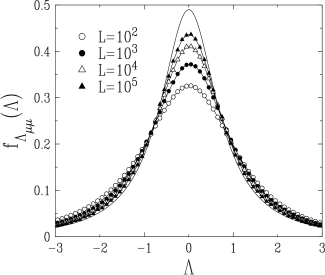
Figure 3: Study of the convergence of the distribution of $S_{L}$ towards the asymptotic scaling law (4.39). Symbols: histograms of numerical data for $\ln(S_{L}/L)$ for $\mu=\nu=0.8$ and four values of the sample length $L$. Solid line: theoretical prediction for the asymptotic distribution of $\Lambda_{\mu\mu}$, equation (4.53).

5 Discussion

In the present work we have studied a model of quantum transport in one dimension based on a disordered array of units whose lengths $\ell_{n}$ and actions $s_{n}$ are independent random variables with either narrow or broad distributions. We have successively investigated the statistical ensemble at fixed number $N$ of units (in Section 3) and the statistical ensemble at fixed sample length $L$ (in Section 4). The model is richer in the latter ensemble than in the former because the sample action $S_{L}$ is the sum of a random rather than fixed number $N_{L}$ of independent random variables. Equation (4.8) has been the starting point of the analysis in the ensemble at fixed sample length. This equation is analogous to the Montroll-Weiss equation [18], which is well-known in the theory of the continuous time random walks. Nevertheless the overlap between the present work and the abundant literature on continuous time random walks (see, e.g., [19]), and more generally on fractional diffusion (see, e.g., [21]), seems to be minute. This is essentially because our basic random variables (lengths and actions) are intrinsically positive whereas most works on fractional diffusion consider displacements which are symmetrically distributed random variables, and so all the results differ. Let us however mention that the distribution of our variable $Y_{\mu\nu}$ appears in some form in Reference [22].

The main outcomes of this work, that is, those concerning the ensemble at fixed sample length derived in Section 4, are summarized in the phase diagram shown in Figure 4. Four different phases can be distinguished, depending on whether the indices $\mu$ and $\nu$ are greater or less than unity. A fluctuating scaling behaviour for the action $S_{L}$, of the form

$$S_{L}\approx a\,Y\,L^{\alpha},$$ (5.1)

has been shown to hold in Phases II, III, and IV. This fluctuating scaling law consists of three factors: a power law $L^{\alpha}$ of the sample length, with a scaling exponent $\alpha$ whose value dictates the localization properties of the eigenstates, as detailed below; a rescaled random variable $Y$, which has a non-trivial asymptotic distribution with some universal character; and a non-universal prefactor $a$, which encompasses the microscopic details of the model. Table 1 gives the expressions of the exponent $\alpha$ and of the rescaled random variable $Y$ in the four phases of the model. Remarkably enough, $Y$ can always be expressed in terms of positive Lévy variables ${\cal L}_{\mu}$.

Figure 4: Phase diagram of the model in the plane of the indices $\mu$ and $\nu$, showing the four phases labelled I to IV. The scaling behaviour of $S_{N}$ and $L_{N}$ at fixed $N$ (Section 3) and of $S_{L}$ at fixed $L$ (Section 4) is given for each phase.

Phase	Indices	$\alpha$	$Y$
I	$\mu>1$, $\nu>1$	1	$1$
II	$\mu<1$, $\nu>1$	$1/\mu$	${\cal L}_{\mu}$
III	$\mu>1$, $\nu<1$	$\nu$	$Z_{\nu}={{\cal L}_{\nu}}^{-\nu}$
IV	$\mu<1$, $\nu<1$	$\nu/\mu$	$Y_{\mu\nu}={\cal L}_{\mu}\,{{\cal L}_{\nu}}^{-\nu/\mu}$

Table 1: Expressions of the exponent $\alpha$ and of the rescaled random variable $Y$ involved in the fluctuating scaling law (5.1) for the sample action $S_{L}$ in the four phases of the model. Phase I: $Y=1$ is trivial, and so $S_{L}$ is self-averaging. Phases II, III, and IV: $Y$ is non-trivial, and so $S_{L}$ is not self-averaging.

The physical consequences of the fluctuating scaling law (5.1) are the following. As recalled in the introduction, in the usual one-dimensional localization problem, where the random potential has short-range correlations, the conductance, which is proportional to the transmission probability $|{{\cal T}}|^{2}$, is a strongly fluctuating quantity in the insulating regime of long enough samples ($L\gg\xi$). On the other hand, the action $S$ is much better behaved, as it is self-averaging in a strong sense. Whenever the fluctuating scaling law (5.1) holds, the action itself is not self-averaging but keeps on fluctuating in samples whose length is arbitrarily large. The same feature holds for the sample-dependent effective localization length, defined as

$$\xi_{L}=\displaystyle{\displaystyle L\over\displaystyle S_{L}},$$ (5.2)

for which (5.1) implies

$$\xi_{L}\approx\displaystyle{\displaystyle L^{1-\alpha}\over\displaystyle a\,Y}.$$ (5.3)

The lack of self-averaging of the action $S_{L}$ and of the effective localization length $\xi_{L}$, which occurs in three of the four phases of the model, is one of its most salient features. As recalled in the introduction, the lack of self-averaging of the action was also observed in the superlocalized regime of one-dimensional models with non-stationary random potentials whose fluctuations grow with distance [10, 11, 12]. We are therefore tempted to argue that a fluctuating scaling behaviour of the form (5.1) is a generic feature of quantum transport in a large universality class of one-dimensional systems with broad disorder, in the sense of random potentials with strong and long-range correlated fluctuations.

Three different regimes of localization are allowed by the fluctuating scaling law (5.1), according to the value of the scaling exponent $\alpha$.

• $\alpha<1$ (Phase IV for $\mu>\nu$ and Phase III): Underlocalization. In this regime the typical sample action $S_{L}$ grows less rapidly than linearly with the sample length $L$. The effective localization length therefore grows with $L$ as the power law $\xi_{L}\sim L^{1-\alpha}$. This underlocalized regime is intermediate between localized and extended. It is qualitatively reminiscent of the behaviour right at the critical point corresponding to the metal-insulator transition in higher dimension.

• $\alpha>1$ (Phase IV for $\mu<\nu$ and Phase II): Superlocalization. In this regime the typical sample action $S_{L}$ grows more rapidly than linearly with the sample length $L$. The effective localization length therefore decreases with $L$ as the power law $\xi_{L}\sim L^{-(\alpha-1)}$. The positive exponent $\alpha-1$ can be arbitrarily large if $\mu\ll 1$. This superlocalized regime is similar to that observed in one-dimensional models with non-stationary random potentials [10, 11, 12]. For such potentials, however, we have $\alpha=1+H/2$, with the Hurst exponent of the random potential satisfying $0<H<1$, and so the value of $\alpha$ cannot be greater than $3/2$.

• $\alpha=1$ (Phase IV for $\mu=\nu$): Fluctuating localization. In this regime the typical sample action $S_{L}$ grows linearly with $L$, just as in the usual one-dimensional localization problem, where the random potential has short-range correlations. However, at variance with the usual situation, the action keeps on fluctuating in samples whose length is arbitrarily large. The effective localization length $\xi_{L}$ also keeps on fluctuating from sample to sample, without ever systematically increasing or decreasing as the sample length is increased. Its probability distribution is indeed asymptotically independent of the sample length. The term of fluctuating localization is therefore fully justified. Equation (4.46) leads to the expression

  $$\xi_{L}\approx\displaystyle{\displaystyle\ell_{0}\over\displaystyle s_{0}Y_{\mu\mu}},$$ (5.4)

  where $Y_{\mu\mu}$ is distributed as the ratio of two Lévy variables with the same index, equation (4.47). Therefore, apart from the prefactor $\ell_{0}/s_{0}$, the effective localization length $\xi_{L}$ is also distributed as the ratio of two Lévy variables with the same index $\mu$, and so its probability density is also given by a Lamperti law (4.49).

Along the borderlines which separate the various phases shown in Figure 4, that is, when at least one of the indices is equal to unity, the above results are affected by logarithmic corrections to scaling. The simplest case occurs in the ensemble at fixed number $N$ of units. The approach of Section 3 leads to the following result in the marginal case $\mu=1$:

$$S_{N}\approx N\,s_{0}\,(\ln N+C+\eta).$$ (5.5)

Here $C$ is a non-universal constant which depends on the whole shape of the probability distribution $f_{s}(s)$ and $\eta$ is a rescaled random variable whose universal probability distribution is characterized by the following moment generating function:

$$\widehat{f}_{\eta}(y)={\rm e}^{y\ln y}.$$ (5.6)

The sample action $S_{N}$ may be called marginally self-averaging, as its mean grows as $N\ln N$ whereas its fluctuations grow as $N$.

Appendix. Scattering and transport in the weak transmission regime

This appendix is devoted to the study of the scattering and transport properties of a single unit and of an array of $N$ units. We first recall the transfer matrix formalism for a single unit [3, 8, 9]. We then use this formalism to obtain the amplitude of transmission through an array of $N$ units in the regime where the transmission through each unit is small. We derive the law of addition for the actions (A.24), which is the starting point of the model investigated in this paper.

A.1 Transfer matrix formalism for a single unit

Let us first consider the scattering of a quantum particle by a single unit. The time-independent Schrödinger equation corresponding to this process is

$$-\psi^{\prime\prime}(x)+V(x)\psi(x)=E\psi(x),$$ (A.1)

where the potential $V(x)$ has an arbitrary form in the scattering unit ($a\leq x\leq b$) and vanishes elsewhere. In both half-lines (perfect leads) on either side of the unit, the wavefunction is a superposition of plane waves $\exp(\pm{\rm i}kx)$, with $k=\displaystyle\sqrt{E}$:

$$\psi(x)=\left\{\matrix{A\,{\rm e}^{{\rm i}kx}+B\,{\rm e}^{-{\rm i}kx}\quad\hfill&{\rm on~{}the~{}left~{}of~{}the~{}unit}\hfill&(x<a),\hfill\cr C\,{\rm e}^{{\rm i}kx}+D\,{\rm e}^{-{\rm i}kx}\hfill&{\rm on~{}the~{}right~{}of~{}the~{}unit}\hfill&(x>b).\hfill}\right.$$ (A.2)

The amplitudes $A$, $B$, $C$, and $D$ are linked together by linear relations of the form

$$\pmatrix{C\cr D}=M\pmatrix{A\cr B},$$ (A.3)

where $M$ is the transfer matrix of the unit. Time reversal invariance implies that $M$ can be parametrized as

$$M=\pmatrix{e&f\cr f^{\star}&e^{\star}},$$ (A.4)

where the star denotes complex conjugation. In addition, conservation of the probability current leads to the condition that

$$\det M=|{e}|^{2}-|{f}|^{2}=1.$$ (A.5)

Let $r$ (resp. $r^{\prime}$) and $t$ (resp. $t^{\prime}$) denote the reflection and transmission amplitudes for a particle coming from the left (resp. right). The first case corresponds to the values $A=1$, $B=r$, $C=t$, and $D=0$, the second to the values $A=0$, $B=t^{\prime}$, $C=r^{\prime}$, and $D=1$. Thus we have

$$t=t^{\prime}=\displaystyle{\displaystyle 1\over\displaystyle e^{\star}},\quad r=-\displaystyle{\displaystyle f^{\star}\over\displaystyle e^{\star}},\quad r^{\prime}=\displaystyle{\displaystyle f\over\displaystyle e^{\star}}.$$ (A.6)

These quantities satisfy the relations

$$|{r}|^{2}=|{r^{\prime}}|^{2}=1-|{t}|^{2},\quad r^{\prime}t^{\star}+r^{\star}t=0.$$ (A.7)

The above relations allow one to derive several equivalent parametrizations of the transfer matrix in terms of the reflection and transmission amplitudes; the one we choose here is the following:

$$M=\pmatrix{1/t^{\star}&-r^{\star}/t^{\star}\cr-r/t&1/t}.$$ (A.8)

A.2 Many units in the weak transmission regime

Let us now consider the transmission through a sample consisting of an arbitrary number $N$ of units which are put end to end. The transfer matrix ${\cal M}_{N}$ of the whole sample is the ordered product of the transfer matrices $M_{n}$ of the units,

$${\cal M}_{N}=M_{N}\cdots M_{1}.$$ (A.9)

This equation is equivalent to the matrix recursion equation

$${\cal M}_{N}=M_{N}{\cal M}_{N-1}.$$ (A.10)

By analogy with the expression (A.8) of the transfer matrix for a single unit, we parametrize ${\cal M}_{N}$ as

$${\cal M}_{N}=\pmatrix{1/{\cal T}_{N}^{\star}&-{\cal R}_{N}^{\star}/{\cal T}_{N}^{\star}\cr-{\cal R}_{N}/{\cal T}_{N}&1/{\cal T}_{N}},$$ (A.11)

where ${\cal R}_{N}$ and ${\cal T}_{N}$ are the reflection and transmission amplitudes corresponding to the whole sample. Equation (A.10) leads to the following non-linear recursion relations:

$${\displaystyle 1\over\displaystyle{\cal T}_{N}}=\displaystyle{\displaystyle 1\over\displaystyle t_{N}{\cal T}_{N-1}}+\displaystyle{\displaystyle r_{N}{\cal R}_{N-1}^{\star}\over\displaystyle t_{N}{\cal T}_{N-1}^{\star}},\quad\displaystyle{\displaystyle{\cal R}_{N}\over\displaystyle{\cal T}_{N}}=\displaystyle{\displaystyle r_{N}\over\displaystyle t_{N}{\cal T}_{N-1}^{\star}}+\displaystyle{\displaystyle{\cal R}_{N-1}\over\displaystyle t_{N}{\cal T}_{N-1}},$$ (A.12)

with the initial conditions ${\cal T}_{0}=1$ and ${\cal R}_{0}=0$. Combining these two relations, we obtain a three-term non-linear recursion relation linking ${\cal T}_{N}$ to ${\cal T}_{N-1}$ and ${\cal T}_{N-2}$, which is

$${\displaystyle 1\over\displaystyle{\cal T}_{N}}=\displaystyle{\displaystyle 1\over\displaystyle t_{N}{\cal T}_{N-1}}+\displaystyle{\displaystyle t_{N-1}r_{N}\over\displaystyle r_{N-1}t_{N}}\left(\displaystyle{\displaystyle 1\over\displaystyle{t_{N-1}^{\star}}{\cal T}_{N-1}}-\displaystyle{\displaystyle 1\over\displaystyle{\cal T}_{N-2}}\right).$$ (A.13)

Setting

$${\cal T}_{N}=\frac{t_{1}\dots t_{N}}{{\cal D}_{N}}$$ (A.14)

and using the second relation of (A.7), we find that ${\cal D}_{N}$ is linked to ${\cal D}_{N-1}$ and ${\cal D}_{N-2}$ by the following linear recursion relation:

$${\cal D}_{N}={\cal D}_{N-1}-\displaystyle{\displaystyle r^{\prime}_{N-1}r_{N}\over\displaystyle 1-{|t_{N-1}|}^{2}}\left({\cal D}_{N-1}-{|t_{N-1}|}^{2}{\cal D}_{N-2}\right).$$ (A.15)

We are interested here in the expression of ${\cal T}_{N}$ in the regime in which the probability of transmission through each unit is small. In this regime, neglecting $|{t_{N-1}}|^{2}$ with respect to unity, (A.15) simplifies to

$${\cal D}_{N}\approx(1-r^{\prime}_{N-1}r_{N}){\cal D}_{N-1},$$ (A.16)

with ${\cal D}_{1}=1$. Iterating this equation, we obtain

$${\cal D}_{N}\approx\prod_{n=1}^{N-1}(1-r^{\prime}_{n}r_{n+1}).$$ (A.17)

We are thus left with the following expression for the transmission amplitude ${\cal T}_{N}$ in the weak transmission regime:

$${\cal T}_{N}\approx\displaystyle{\displaystyle\prod_{n=1}^{N}t_{n}\over\displaystyle\prod_{n=1}^{N-1}(1-r^{\prime}_{n}r_{n+1})}.$$ (A.18)

This leading order result is valid up to corrections which are proportional to the $|{t_{n}}|^{2}$ in relative value and could be derived from the full recursion relation (A.15). The result (A.18) can be recast in the following more appealing way:

$${\cal T}_{N}\approx t_{1}\,\displaystyle{\displaystyle 1\over\displaystyle 1-r^{\prime}_{1}r_{2}}\,t_{2}\,\displaystyle{\displaystyle 1\over\displaystyle 1-r^{\prime}_{2}r_{3}}\,t_{3}\dots t_{N-1}\,\displaystyle{\displaystyle 1\over\displaystyle 1-r^{\prime}_{N-1}r_{N}}\,t_{N}.$$ (A.19)

Here each denominator corresponds to the geometric resummation of all the repeated reflections between two consecutive units. These are indeed the only internal reflections from the whole multiple scattering expansion that survive at leading order in the weak transmission regime.

The leading order expression of the sample action is therefore

$$S_{N}=-{\textstyle{\frac{1}{2}}}\ln|{{\cal T}_{N}}|^{2}\approx-{\textstyle{\frac{1}{2}}}\sum_{n=1}^{N}\ln|{t_{n}}|^{2}+\mathop{{\rm Re}}\sum_{n=1}^{N-1}\ln(1-r^{\prime}_{n}r_{n+1}),$$ (A.20)

i.e.,

$$S_{N}\approx\sum_{n=1}^{N}s_{n}+\mathop{{\rm Re}}\sum_{n=1}^{N-1}\ln\left(1-{|{r_{n}}|}{|{r_{n+1}}|}\,{\rm e}^{{\rm i}(\theta^{\prime}_{n}+\theta_{n+1})}\right),$$ (A.21)

where we have introduced the action $s_{n}$ and the reflection angles $\theta_{n}$ and $\theta^{\prime}_{n}$ of each unit, according to

$$s_{n}=-{\textstyle{\frac{1}{2}}}\ln|{t_{n}}|^{2},\quad r_{n}=|{r_{n}}|{\rm e}^{{\rm i}\theta_{n}},\quad r^{\prime}_{n}=|{r_{n}}|{\rm e}^{{\rm i}\theta^{\prime}_{n}}.$$ (A.22)

We now introduce our second hypothesis besides the weak transmission regime, namely that the internal reflection angles $\theta_{n}$ and $\theta^{\prime}_{n}$ are random and uniformly distributed between $0$ and $2\pi$. This hypothesis can be postulated as a mere simplifying assumption, in keeping with a long tradition in localization theory [4, 3, 6, 23]. It can alternatively be justified on physical grounds by considering that the reflection angles are rapidly varying functions of the incoming momentum $k$. This is especially true in the weak transmission regime, in which the length $\ell_{n}$ of each unit is expected to be such that $k\ell_{n}\gg 1$. As a consequence, any narrow distribution of incoming momentum will result in a uniform averaging over the reflection angles. Carrying out this averaging over the angles $\theta_{n}$ and $\theta^{\prime}_{n}$ in (A.21), we find that the second sum vanishes by virtue of the identity

$$\int_{0}^{2\pi}\ln(1-z\,{\rm e}^{i\theta})\,{\rm d}\theta=-\sum_{k\geq 1}\displaystyle{\displaystyle z^{k}\over\displaystyle k}\underbrace{\int_{0}^{2\pi}{\rm e}^{ik\theta}\,{\rm d}\theta}_{\displaystyle 2\pi\,\delta_{k0}}=0,$$ (A.23)

which holds for any number $z$ such that $|{z}|\leq 1$.

We thus find that the action $S_{N}$ of the whole sample is approximately given by

$$S_{N}\approx\sum_{n=1}^{N}s_{n}.$$ (A.24)

This simple formula, which can be referred to as the law of addition for the actions, is the starting point of the model investigated in this paper.

References

References

- [1] Lifshitz I M, Gredeskul S A and Pastur L A 1988 Introduction to the Theory of Disordered Systems (New York: Wiley)
- [2] Kramer B and MacKinnon A 1993 Rep. Prog. Phys. 56 1469
- [3] Pendry J B 1994 Adv. Phys. 43 461
- [4] Landauer R 1970 Phil. Mag. 21 863
- [5] Imry Y and Landauer R 1999 Rev. Mod. Phys. 71 S306 and references therein
- [6] Anderson P W, Thouless D J, Abrahams E and Fisher D S 1980 Phys. Rev. B 22 3519
- [7] Abrikosov A A 1981 Solid State Commun. 37 997
- [8] Crisanti A, Paladin G and Vulpiani A 1992 Products of Random Matrices in Statistical Physics (Berlin: Springer)
- [9] Luck J M 1992 Systèmes désordonnés unidimensionnels (Collection Aléa-Saclay)
- [10] de Moura F A B F and Lyra M L 1998 Phys. Rev. Lett. 81 3735 —– 1999 Physica A 266 465 —– 2000 Phys. Rev. Lett. 84 199
- [11] Kantelhardt J W, Russ S, Bunde A, Havlin S and Webman I 2000 Phys. Rev. Lett. 84 198 Bunde A, Havlin S, Kantelhardt J W, Russ S and Webman I 2000 J. Mol. Liq. 86 151 Russ S, Kantelhardt J W, Bunde A and Havlin S 2001 Phys. Rev. B 64 134209
- [12] Luck J M 2005 J. Phys. A 38 987
- [13] Cox D R 1962 Renewal Theory (London: Methuen) Cox D R and Miller H D 1965 The Theory of Stochastic Processes (London: Chapman & Hall)
- [14] Gradshteyn I S and Ryzhik I M 1965 Table of Integrals, Series, and Products (New York and London: Academic Press)
- [15] Godrèche C and Luck J M 2001 J. Stat. Phys. 104 489
- [16] Lévy P 1954 Théorie de l’addition des variables aléatoires (Paris: Gauthier-Villars) Gnedenko B V and Kolmogorov A N 1954 Limit Distributions for Sums of Independent Random Variables (Reading MA: Addison-Wesley)
- [17] Bouchaud J P and Georges A 1990 Phys. Rep. 195 127 Shlesinger M F, Zaslavsky M G and Frisch U 1995 Lévy Flights and Related Topics in Physics Lecture Notes in Physics 450 (Berlin: Springer)
- [18] Montroll E W and Weiss G H 1965 J. Math. Phys. 6 167
- [19] Hughes B D 1995 Random Walks and Random Environments Volume 1: Random Walks (Oxford: Oxford University Press)
- [20] Lamperti J 1958 Trans. Amer. Math. Soc. 88 380
- [21] Metzler R and Klafter J 2000 Phys. Rep. 339 1 —– 2004 J. Phys. A 37 R161
- [22] Saichev A I and Zaslavsky G M 1997 Chaos 7 753
- [23] Abrahams E and Stephen M 1980 J. Phys. C 13 L377