Discovery of a bright eclipsing cataclysmic variable

Abstract

Aims. We report on the discovery of J0644+3344, a bright deeply eclipsing cataclysmic variable (CV) binary.

Methods. Optical photometric and spectroscopic observations were obtained to determine the nature and characteristics of this CV.

Results. Spectral signatures of both binary components and an accretion disk can be seen at optical wavelengths. The optical spectrum shows broad H I, He I, and He II accretion disk emission lines with deep narrow absorption components from H I, He I, Mg II and Ca II. The absorption lines are seen throughout the orbital period, disappearing only during primary eclipse. These absorption lines are either the the result of an optically-thick inner accretion disk or from the photosphere of the primary star. Radial velocity measurements show that the H I, He I, and Mg II absorption lines phase with the the primary star, while weak absorption features in the continuum, between H$\alpha$ and H$\beta$, phase with the secondary star. Radial velocity solutions give a 150$\pm$4 km s^-1 semi-amplitude for the primary star and 192.8$\pm$5.6 km s^-1 for the secondary, resulting in a primary to secondary mass ratio of $q$=1.285. The individual stellar masses are 0.63$-$0.69 M_⊙ for the primary and 0.49$-$0.54 M_⊙ for the secondary, with the uncertainty largely due to the inclination.

Conclusions. The bright eclipsing nature of this binary has helped provide masses for both components with an accuracy rarely achieved for cataclysmic variables. This binary most closely resembles a nova-like UX UMa or SW Sex type of cataclysmic variable. J0644+3344, however, has a longer orbital period than most UX UMa or SW Sex stars. Assuming an evolution toward shorter orbital periods, J0644+3344 is therefore likely to be a young interacting binary. The secondary star is consistent with the size and spectral type of a K8 star, but has the mass of a M0.

1 Introduction

Cataclysmic Variables (CVs) are close binary systems consisting of a white dwarf (WD) primary and late type secondary which overflows its Roche lobe. In these systems, mass is transfered from the secondary onto the primary star, often forming an accretion disk. CVs are thought to have been produced through the common-envelope (CE) process. In the CE process, one component of a binary star system has a rapidly expanding envelope, evolving on either the red giant branch (RGB) or the asymptotic giant branch (AGB). The giant fills its Roche lobe starting rapid mass transfer, quickly filling its companion’s Roche lobe as well. The companion star spirals in helping to eject the envelope which has formed around both stars. The initial conditions of the binary and the efficiency of ejecting the envelope determine the final separation of the binary. After the ejection of the envelope, the core of the giant is left behind which has formed into either a subdwarf or white dwarf, while the secondary’s mass remains nearly unchanged. Those post-CE systems which have not coalesced are thought to then go through a detached phase, where further orbital angular momentum is lost through gravitational radiation and magnetic braking. Post-common envelope systems that have evolved to the point where the secondary’s Roche-lobe is filled, either by the secondary evolving off of the main sequence, or by loss of orbital angular momentum and favorable mass ratios, then become CVs. There are approximately 28 known post-common envelope systems which are also believed to be pre-CVs (Sing 2005).

Although the accretion disk usually dominates the optical continuum out-shining the primary, the white dwarf primary can be observed if it is sufficiently hot or in cases of low mass transfer. The masses, radii, and spectral line profiles measured for the primary star in CVs have thus far all been consistent with white dwarf characteristics. Certain nova-like (NL) CVs were previously thought to contain a hot subdwarf, such as UX UMa (Walker & Herbig 1954), because of the appearance of broad absorption lines. These CVs, however, were shown to contain optically thick inner accretion disks which gives rise to the broad absorption features.

We present discovery observations of a new bright NL CV NSVS07178256 (hereafter J0644). We identified this system as a variable star while conducting an extensive search campaign for short period eclipsing binaries among objects in the Northern Sky Variability Survey (NSVS, Wozniak 2004) photometry database. The coordinates for J0644 are included in Table 1 along with a finder chart in Fig. 1. The NSVS database was searched for periodicities by simultaneously using the String-Length (Clarke 2002) and Analysis of Variance (Schwarzenberg-Czerny 1989) methods. J0644 revealed itself as a possible candidate having strong photometric variations exceeding one magnitude, interpreted as brief periodic eclipses occurring with a period of 0.538669 days.

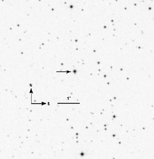
Figure 1: Digital Sky Survey (Poss II, blue) finding chart for J0644+3344.

There are no previous references to this binary in the literature outside of our initial observations (Sing 2005). The only initial estimation that we had of its apparent magnitude was the I-band value provided by the NSVS ($I_{NSVS}\sim 13.4$). A more careful search on this object revealed that it can be identified with the ROSAT All Sky Survey source 1RXS J064434.5+334451. The object also appears in the 2MASS catalog as object 2MASS J06443435+3344566 (J=12.493 $\pm$ 0.023; H=12.163 $\pm$ 0.026; Ks=12.03 $\pm$ 0.022). The J-Ks, J-H, and H-Ks colors from 2MASS (J-Ks=0.463 $\pm$ 0.032; J-H=0.330 $\pm$ 0.035, and H-Ks = 0.133 $\pm$ 0.034) provide the first clues about the nature of this binary. From the UCAC2 catalog (Zacharias et. al. 2004), we find that J0644 has a small proper motion ($\mu_{a}$= -5 $\pm$ 4.3; $\mu_{d}$= -3.3 $\pm$ 1.7)

Its H-Ks color is consistent with the system being a low-mass eclipsing binary, however its J-H color is too blue due to the disk contribution (J-H $>$ 0.5 for low-mass stars). Placing this binary in the (J-H) vs (H-Ks) diagrams for CVs (Hoard et al. 2002) suggested that J0644 had the characteristics of a NL CV.

We obtained new photometric and spectroscopic observations of J0644 in an attempt to identify the nature of the binary system, refine its orbital period, and perform radial velocity measurements to allow estimation of the component masses. We describe these observations in §2, analyze the data in §3, discuss the results in §4, and present our conclusions in §5.

Table 1: J0644+3344 System Parameters

Parameter	Value	Value
RA(2000)	06:44:34.637
DEC(2000)	+33:44:56.615
U	13.11 $\pm$0.07
B	13.84 $\pm$0.05
V	13.56 $\pm$0.24
R	13.29 $\pm$0.05
I	12.8 $\pm$0.1
J	12.493$\pm$0.023	2MASS
H	12.163$\pm$0.026	2MASS
K	12.03 $\pm$0.022	2MASS
ROTSE magnitude	13.392	Unfiltered
Secondary	K8 (Spectral Type)	M0 (Mass)
$K_{P}$ Velocity	150 $\pm$ 4 km s-1	He II solution
$K_{2}$ Velocity	192.8 $\pm$ 5.6 km s-1
$\gamma$ system	-7.1 $\pm$ 1.3 km s-1
$M_{P}(i)$	0.63$-$0.69 M⊙	Mass range
$M_{2}(i)$	0.49$-$0.54 M⊙	Mass range
$a(i)$	1.82-1.88 R⊙
$i$	$>$ 76∘	Inclination

2 Observations

2.1 Kuiper 1.55m Photometry

Time resolved differential photometry of J0644+3344 (Table 2) was obtained in February, March, November and December of 2005 and in January and October of 2006 at the Steward Observatory 1.55m (61” Kuiper) Telescope located on Mt. Bigelow. Most of the early 2005 observations were taken with a NSF Lick3 2048$\times$2048 pixel CCD, for which the image scale of 0.15^′′ pixel${-1}$ allowed a 5.1^′$\times$5.1^′ field of view. A new facility imager with a blue-sensitive dual-amplifier Fairchild 4096$\times$4096 CCD was introduced in September 2005, expanding the available field of view to 10.2^′$\times$10.2^′. With both instruments, 3$\times$3 pixel on-chip binning was utilized to substantially improve the readout time. The average overhead times between successive images in a single filter were 26 s and 23 s for the 2K and 4K CCD’s, respectively. Each filter change required an additional 10 s with the 2KCCD, or 6 s with the 4KCCD. On the nights for which two filters are listed in Table 2, the filters were alternated for the entire observation period. The sampling times can be calculated using the overhead values plus the exposure times in Table 2. For example, the sampling time was 71 s for the 04 Feb 2005 data, and it was 133 s between two exposures in the same filter on 06 Jan 2006.

The data were reduced using standard IRAF routines for bias subtraction, flat-fielding, and cosmic ray cleaning. Precise differential photometry was obtained using IRAF’s APPHOT package to measure the magnitude of J0644+3344 relative to the mean magnitudes of a set of eight to ten comparison stars in each image. The size of the stellar aperture radius (2.25 times the observed stellar FWHM) and the background sky annulus (four times the area of the star aperture with an inner boundary of 5.0 times the stellar FWHM) were held constant for all stars in a given image, although the values varied from image to image, according to the seeing. An upper limit to the aperture radius of 4.5^′′ was imposed for the few occasions when the image FWHM’s were greater than 2.0^′′, to avoid any contamination from a faint visual companion 6.5^′′ SSE of J0644+3344.

There was occasional cirrus during several of the nights when J0644+3344 was observed. The effect on the relative photometry was minimal, however, due to our rather long exposures and the selection of fairly bright reference stars. Differential light curves for one of the comparison stars relative to the mean of all the others indicates that the typical 1 $\sigma$ noise in the J0644+3344 light curves was 0.001 to 0.003 magnitudes whenever the extinction due to clouds was less than 0.1–0.2 mags. For cloud extinctions up to 1.0 magnitudes, the noise in the relative light curves increased to approximately 0.01 mag. The observations were halted whenever there was a drop of more than one magnitude due to clouds.

Stars in the field of J0644+3344 were calibrated using Landolt (1992) UBVRI standards during the clear nights of 06 Dec 2005 and 05 Mar 2006. A description of the photometric solutions can be found in Appendix I. Table 3 contains a list of the comparison stars used and their magnitudes. The absolute photometry of the comparison stars and the derived extinction coefficients for Mt. Bigelow were used to correct all of the J0644+3344 light curves to the standard system.

Table 2: Log of Kuiper 1.55m Photometric observations.

UT date	HJD Start	HJD End	Filters	N	Inst.
02 Feb 05	3403.63100	3403.86903	R	300	4K
04 Feb 05	3405.61762	3405.87962	R	319	2K
01 Mar 05	3430.60707	3430.80255	R+B	203	2K
02 Mar 05	3431.59528	3431.83146	R+B	256	2K
03 Mar 05	3432.60205	3432.79780	R+B	209	2K
04 Nov 05	3678.81874	3679.03925	R	338	4K
05 Nov 05	3679.78777	3680.03462	B	343	4K
06 Nov 05	3680.85072	3681.03434	B	255	4K
05 Dec 05	3709.71712	3710.04482	R+B	429	4K
06 Dec 05	3710.71717	3711.01314	R+B	305	4K
07 Dec 05	3711.70199	3712.01251	R+B	406	4K
08 Dec 05	3712.69835	3713.03623	R+B	445	4K
06 Jan 06	3741.63524	3741.29503	R+B	412	4K
07 Jan 06	3742.62904	3742.95755	U+I	410	4K
10 Jan 06	3745.60197	3745.95607	V+R	452	4K
13 Oct 06	4021.91698	4022.02386	B	109	4K

Table 3: J0644+3344 Field Reference Stars

Object	RA	DEC	V	U-B	B-V	V-R	V-I	n	m
	(J2000)	(J2000)						obs.	nights
J0644	06:44:34.4	+33:44:57	13.564$\pm$0.243	-0.732$\pm$0.065	0.279$\pm$0.053	0.274$\pm$0.057	0.780$\pm$0.099	3	2
J0644-A	06:44:20.4	+33:40:06	11.599$\pm$0.006	0.375$\pm$0.006	0.823$\pm$0.001	0.397$\pm$0.034	-	2	1
J0644-B	06:44:57.0	+33:40:29	14.219$\pm$0.002	0.141$\pm$0.008	0.766$\pm$0.001	0.436$\pm$0.001	-	2	1
J0644-C	06:44:33.0	+33:41:12	11.925$\pm$0.006	0.817$\pm$0.003	1.113$\pm$0.006	0.506$\pm$0.040	-	2	1
J0644-D	06:44:34.1	+33:42:07	14.704$\pm$0.023	0.108$\pm$0.001	0.656$\pm$0.006	0.360$\pm$0.008	0.705$\pm$0.013	3	2
J0644-E	06:44:25.9	+33:42:53	13.594$\pm$0.022	0.497$\pm$0.005	0.934$\pm$0.005	0.491$\pm$0.006	0.972$\pm$0.011	3	2
J0644-F	06:44:27.1	+33:44:23	15.923$\pm$0.018	0.039$\pm$0.006	0.436$\pm$0.007	0.253$\pm$0.011	0.542$\pm$0.020	3	2
J0644-G	06:44:15.3	+33:44:57	14.043$\pm$0.019	0.107$\pm$0.016	0.661$\pm$0.014	0.372$\pm$0.014	0.708$\pm$0.020	1	1
J0644-H	06:44:37.1	+33:45:17	15.529$\pm$0.006	0.097$\pm$0.010	0.660$\pm$0.013	0.369$\pm$0.008	0.750$\pm$0.015	3	2
J0644-I	06:44:29.1	+33:45:19	14.499$\pm$0.014	0.959$\pm$0.009	1.170$\pm$0.009	0.590$\pm$0.010	1.159$\pm$0.017	3	2
J0644-J	06:44:30.0	+33:45:51	15.619$\pm$0.013	0.160$\pm$0.001	0.744$\pm$0.010	0.409$\pm$0.014	0.816$\pm$0.024	3	2
J0644-K	06:44:20.2	+33:45:58	15.567$\pm$0.010	-0.058$\pm$0.012	0.559$\pm$0.013	0.309$\pm$0.005	0.656$\pm$0.009	3	2
J0644-L	06:44:59.1	+33:46:13	13.298$\pm$0.002	-0.007$\pm$0.008	0.647$\pm$0.004	0.347$\pm$0.002	-	2	1
J0644-M	06:44:33.9	+33:46:20	14.767$\pm$0.004	0.227$\pm$0.003	0.765$\pm$0.008	0.418$\pm$0.008	0.826$\pm$0.014	3	2
J0644-N	06:44:27.6	+33:46:55	14.006$\pm$0.004	1.619$\pm$0.005	1.465$\pm$0.010	0.752$\pm$0.008	1.449$\pm$0.014	3	2
J0644-P	06:44:57.2	+33:47:46	13.679$\pm$0.001	1.095$\pm$0.012	1.220$\pm$0.002	0.598$\pm$0.006	-	2	1
J0644-Q	06:44:17.7	+33:47:43	14.162$\pm$0.007	0.066$\pm$0.008	0.658$\pm$0.014	0.334$\pm$0.013	0.703$\pm$0.022	3	2
J0644-R	06:44:34.8	+33:47:52	13.026$\pm$0.004	-0.020$\pm$0.007	0.562$\pm$0.003	0.298$\pm$0.006	0.604$\pm$0.011	3	2
J0644-S	06:44:47.4	+33:48:33	12.972$\pm$0.003	0.000$\pm$0.013	0.381$\pm$0.001	0.196$\pm$0.008	0.416$\pm$0.013	3	2

2.2 Spectroscopic and Spectropolarimetric Observations with the 2.3m Bok Telescope

Spectroscopic observations of J0644 covering multiple orbital cycles were obtained on the Steward Observatory 2.3m Bok telescope, located on Kitt Peak, during 2005 January 16-17, 2005 December 04-07, and 2006 January 09 (see Table 3). The optical spectra were obtained using the Boller and Chivens Spectrograph at the Ritchey-Chretien f/9 focus using multiple grating settings along with a 1200$\times$800 15 $\mu m$ pixel CCD. For 2005 January observations, we used a 1st order 600 line/mm grating blazed at 3568 Å. With a 2.5 arcsec slit width, a typical spectral resolution of 5.5 Å was achieved at a reciprocal dispersion of 1.87 Å/pixel on the CCD. Typical exposure times of 300 seconds yielded characteristic S/N ratios of $60-70$. The 2005 December and 2006 January observations were taken with the 832 line/mm grating and used in 2nd order at two different grating tilts to cover the blue region ($\sim$ $3800-4850$ Å) and 1st order in conjunction with a UV filter to cover the red region ($\sim$ $5000-7000$ Å) with two separate grating tilts. A 1.5 arcsec slit was used producing a typical spectral resolution of 1.8 Å. Before each observation, the instrument was rotated to align the slit perpendicular to the horizon, minimizing the effects of atmospheric dispersion.

Standard IRAF routines were used to reduce the data. The wavelength calibration was established with He-Ar arc-lamp spectra, interpolated between exposures taken before and after each observation, to account for any small wavelength shifts that may occur while the telescope tracks an object. The spectra were flux calibrated using the Massey et al. (1988) spectrophotometric standards G191-B2B and BD+28^∘ 4211, observed over a range of zenith angles covering the program stars’ airmass range.

Spectropolametric observations of J0644 were also taken with the 2.3m Bok telescope using the instrument SPOL (Schmidt et al. 1992) on 2005 Dec 31. The observations covered the region from $4200-8400$ Å  with a resolution of 16 Å. A 2 hour interval between binary phases $0.45-0.75$ (as determined below) were observed. These observations, however, showed no significant signs of circular polarization with a polarimetric fraction of +0.003$\pm$0.003%. The lack of polarization would appear to rule out J0644 as being a polar or intermediate-polar type of CV as the typical magnetic fields would have easily been detected.

Table 4: Log of Spectroscopic and Spectropolarimetric Observations with the 2.3m Bok Telescope

Date	MHJD Start	MHJD End	Spec. Range	N
2005 Jan. 16		3387.2321	Blue	1
2005 Jan. 16	3388.2599	3388.3950	Blue	4
2005 Dec. 04	3709.2061	3709.5283	Blue	38
2005 Dec. 05	3710.2056	3710.5262	Red	37
2005 Dec. 06	3711.1840	3011.5262	Blue	46
2005 Dec. 07	3712.1995	3012.5306	Red	40
2005 Dec. 31	3735.2401	3735.3214	Spol	9
2006 Jan. 09	3745.1532	3745.4544	Red	28

Blue: 3880 - 5040 Å; Red: 5500 - 6200 Å; Spol: spectropolametric

Figure 2: R and B photometry showing the eclipse of the primary star. The points at the bottom of the plot are the R residuals for the 2005 March 02 data which characterize the standard differential photometry errors.

3 Analysis

3.1 Photometry

Photometric coverage in the B and R bands show deep 1 to 1.2 magnitude primary eclipses of the hot primary star (see Fig. 2). The eclipse lasts around 1.3 hours and has a characteristic “V” shape. There also is considerable ’flickering’ in the light curve, indicative of mass transfer, but no evidence of a secondary eclipse. With multiple night coverage of J0644, the fundamental orbital period of the system was subsequently determined to be $P$= 6.4649808$\pm$ 0.0000060 hrs. We define phase 0.0 to be the red-to-blue crossing of the primary star, such that primary eclipse happens at phase 0.0. The current ephemeris for primary eclipse is given by:

$$T_{\mathrm{mid-eclipse}}=HJD(2453403.62501)+(0.26937431)\times E,$$ (1)

with associated errors of $\pm$0.00022 days in T₀ and $\pm 2\times 10^{-7}$ days in $P$.

Although there is a strong He II $\lambda$4686 emission line, part of which is usually associated with a “hot spot” on the accretion disk, we see very little, if any, photometric evidence for a “hot spot” modulation in the light curve. The lack of a noticeable “hot spot” modulation in the light curve, directly before eclipse, is typical of NL CVs. The large, bright accretion disk, combined with the fact that the stream material does not fall deep into the white dwarf potential well before it hits the disk edge, combine to make a low contrast of the “hot spot” with respect to the approximately constant out of eclipse light from the accretion disk.

During the course of our observations (Tables 1-4) as well as the time period covered by the ROTSE observations (2 October 1999 to 29 March 2000) no dwarf nova-type outburst has been observed. The constant out of eclipse brightness and lack of outburst observations is consistent with J0644 being a NL type CV.

3.2 Spectroscopy

Spectroscopically, the out-of-eclipse observations show a strong blue continuum, on which are superimposed broad emission lines due to H I and He I which have a deep, narrow absorption component not easily seen at lower resolution, Fig. 3. At higher resolution, however, the absorption component is resolved, see Fig 4. The strong emission line, He II $\lambda$4686, has no resolved absorption feature and requires a very high level of excitation at its formation site in the accretion disk. Note that strong He II lines occur in both polars (highly magnetic CVs) and in high $\dot{M}$, longer period CVs. About 1/3 of the CVs known with strong He II $\lambda$4686 emission lines are non-magnetic (Szkody et al. 1990).

Figure 3: Optical spectra of J0644+3344 both in eclipse (bottom) and out (top), showing the H I Balmer series, He I, and He II as well as possible Fe II (Mason & Howell 2005). A ’Bowen fluorescence’ feature is also visible at $\lambda$4640 Å  caused by ionized carbon and nitrogen.

Figure 4: Optical spectra of J0644+3344 before primary eclipse (top), during ingress (middle), and at total primary eclipse. Notice, compared to Fig. 3 the absorption lines are fully resolved and can easily be seen.

3.3 Line Flux

The He II $\lambda$4686 emission line flux is seen to modulate on time scales equal to the orbital period, with its value dramatically decreasing during primary eclipse. This would argue that most of the He II emission originates from an inner disk line forming region near the primary star and not in an outer accretion disk hot-spot (see Fig. 5). The emission is not entirely eclipsed, however, suggesting that at least part of the He II emission arises outside of a small inner disk line forming region and/or in the hot-spot. Furthermore, the FWHM of the He II line is seen to decrease by $\sim$70% during eclipse as would be expected when emission from an inner accretion disk with higher Keplerian velocity is eclipsed, decreasing the emission line width.

Figure 5: 2005 Dec 04 & 06 average line flux from the He II $\lambda$4686 emission line. The flux is seen to be at a minimum during primary eclipse at phase 0.0. This would suggest most the emission comes from a hot inner line forming region.

A flux curve of the H I emission line flux for H$\gamma$ is seen in Fig. 6 produced by averaging the Dec 04 and 06 2005 data. This line, while out of eclipse, is comprised of a broad emission line component associated with the accretion disk and a narrow absorption component which can reach well below the continuum (see Fig. 4 & Fig. 7). The line flux is summed over both the absorption and emission line components, making it possible to track the full emission component’s relative contribution to the flux during primary eclipse. The flux also provides information on the component’s line formation location. When the eclipse begins at phase $-$0.15, point A in Fig. 6, the H$\gamma$ flux is seen to abruptly decrease, implying the emission line forms in the outer accretion disk. The flux continues to decrease up until phase $-$0.07, point B, at which point the flux is observed to dramatically increase up to phase $-$0.02, point C. During this ingress period of the eclipse, between points B and C, the central accretion region & primary star are being eclipsed, thus hiding the absorption line component and increasing the H$\gamma$ flux. The spectra change from a blue continuum dominated by deep absorption cores, to a fainter flat continuum containing only emission lines at phase $-$0.02, point C. At this phase, the H I emission is seen to be at its maximum and the primary star and inner accretion disk are eclipsed. The narrow absorption core returns at phase 0.03, point D, lowering the flux which decreases until phase 0.09, point E, when the primary eclipse ends. The time between points B & C is 20.7 minutes, which we use to estimate the radius of the absorption line region (see §3.6).

Figure 6: Average line flux from the H$\gamma$ line using the 2005 Dec 04 & 06 data.

The Balmer decrement provides information about the temperature and density of the emission line forming gas as well as its opacity. It is defined as the ratio between any two H I line intensities, D${}_{\nu}(H\alpha/H_{\beta})=I_{\nu}(H\alpha)/I_{\nu}(H\beta)$. When determining the Balmer decrement from spectra, where fluxes are measured, the direct comparison of flux-ratios to intensity-ratios assumes that the measured emission lines have the same profiles (see Mason et al. 2000 and references therein). The Balmer emission lines of J0644 are complex due to the absorption line components, changing the line profile in a non-uniform manner. The emission lines in eclipse, however, have no absorption line cores and have similarly broadened profiles, making a measurement of D_ν more reliable. Measuring the flux-ratio centered on primary eclipse gives a value of D${}_{\nu}(H\gamma/H\beta)=0.91$. Williams (1991) modeled the Balmer decrement for H I emission lines from accretion disks using grids of temperature, density and inclination. Although D_ν alone does not provide a unique solution for the accretion disk temperature or density, it can provide valuable ranges for those parameters. Seen in Fig. 8, our eclipse measured Balmer decrement corresponds to a number density range between log N_o=$12.8-13.8$ and a temperature range between 8,000 and 15,000 K. The presence of He II in the accretion disk would suggest that an upper temperature range between 10,000 and 15,000 K is more realistic for some portions of the disk, indicative of a hot, NL accretion disk. Using this upper temperature range, the line forming region density is limited to log N_o=$12.8-12.9$.

Figure 7: 2005 December 04 (left) and 06 (right) spectra of J0644+3344.

Figure 8: Balmer decrement (H_γ/H_β) vs. log density (g cm^-3) for four different temperatures calculated by Williams (1991). The values are for an inclination of 80^∘, except for 6,000 K which is calculated at 52^∘. The value measured for J0644+3344 (H_γ/H_β=0.91) is shown as a horizontal line.

3.4 Primary Star Radial Velocities

Radial velocity measurements were performed on the H I and He I absorption lines as well as the H I, He I, and He II emission lines using the 2005 December and 2006 January 2.3m Bok telescope observations. The spectra were velocity shifted to a heliocentric rest frame where the HJD of the midpoint of each exposure was calculated. The radial velocities were measured using a center-of-wavelength, $\lambda^{\prime}$, for each line profile to calculate a Doppler velocity. For each line profile of interest, $\lambda^{\prime}$ was estimated following the formula, $\lambda^{\prime}=\frac{\sum\lambda f_{\lambda}}{\sum f_{\lambda}}$. We assumed a circular orbit and then fit the radial velocity curves with a sine function of the form,

$$V(t)=\gamma+K\sin{\left[2\pi\frac{(t-T_{0})}{P}-2\pi\phi\right]},$$ (2)

using a gradient-expansion algorithm to compute a non-linear least squares fit. The fitted parameters were; the system velocity $\gamma$ , the stellar Keplerian velocity $K$, and the phase offset$\phi$. The photometric ephemeris was used, where $\phi_{0}=0.0$ corresponds to primary eclipse.

The absorption lines of H I, He I, and Mg II (see Fig. 9) are seen to phase with the primary star. The sine fits over the entire period produce $K$ velocities between $150-180$ km s^-1 for the absorption lines. Between phases $-$0.5 to 0, the velocity curve appears sinusoidal, producing better sinusoid fits and larger amplitudes, but then remains approximately constant between phases 0.0 and 0.5 (see Fig 10 and Table 5). There appears to be no clear reason for the flat velocity curve, but curiously, the secondary star’s velocity curve exhibits the same phenomena (see §3.5). A few possible causes of a flat velocity curves may be emission and absorption line blending, magnetic effects, non-uniform disk emission, or effects from an accretion stream.

The emission lines of H I, He I, and He II are also seen to phase with the primary star. The radial velocity curve derived from the He II emission line is seen in Fig 11. This line is single-peaked and is sinusoidal throughout the orbital period, possibly providing a much more precise measure of the $K$ velocity than the H I and He I emission lines. The He II velocity curve gives a $K_{\mathrm{HeII}}$=151$\pm$5 km s^-1 and $\gamma$=-96$\pm$3 km s^-1. The He II emission line appears, therefore, to be the only velocity feature that is observed to behave sinusoidally throughout the entire orbital phase. As we have seen, the bulk of the He II emission arises in the inner-accretion disk which should accurately follow the center of mass of the primary star. No significant phase lags are observed in any of the emission or absorption line velocity solutions (see Table 5). We use the He II velocity solution, $K_{\mathrm{HeII}}$, as the best fit for the $K$ velocity of the primary star, $K_{P}$.

Table 5: J0644+3344 radial velocities fitting over the entire phase (top half) and over phases -0.5 to 0 (bottom half).

Feature	$K$	Phase Offset	$\gamma$	$\chi_{\nu}^{2}$
	km s-1	$\phi-\phi_{phot}$	km s-1
He I $\lambda$4026	189$\pm$6	0.038$\pm$0.005	26$\pm$4	4.25
He I $\lambda$4471	145$\pm$2	0.043$\pm$0.002	5$\pm$1	12
Mg II $\lambda$4481	169$\pm$4	0.045$\pm$0.004	32$\pm$3	4.93
He II $\lambda$4686	150$\pm$4	0.043$\pm$0.004	-95$\pm$3	1.22
He I $\lambda$4026	209$\pm$20	0.033$\pm$0.006	11$\pm$16	2.27
He I $\lambda$4471	266$\pm$8	0.026$\pm$0.002	-73$\pm$6	5.84
Mg II $\lambda$4481	257$\pm$17	0.015$\pm$0.004	-29$\pm$13	4.18
He II $\lambda$4686	167$\pm$14	0.039$\pm$0.007	-104$\pm$10	1.06

The best fit $\gamma$ velocities, measured from both the emission and absorption lines, give widely different values ranging from $\sim$-100 to 25 km s^-1. These differences are similar to those typically seen in CVs such as the dwarf novae WZ Sge (Mason et al. 2000) and VY Aqr (Augusteijn 1994). The velocity differences would suggest that the accretion disk emission is non-symmetric, which leads to the inconsistencies observed.

Figure 9: Radial velocity curve of the He I $\lambda$4471 Å absorption line. Overplotted is a sinusoidal fit over the entire period (solid line), and using only phases -0.5 to 0 (dashed line) which produces a better fit.

Figure 10: Radial velocity measurements of J0644+3344 using the Mg II absorption line plotted against the orbital phase. The velocity variations of Mg II phase with the primary star. Overplotted is a sinusoidal fit over the entire period (solid line), and using only phases -0.5 to 0 (dashed line) which produces a better fit.

Figure 11: Radial velocity measurements of J0644+3344 using the He II emission line.

3.5 Secondary Star Radial Velocities

The 2005 December 07 and 2006 January 09 observations, taken with a first order 1200/mm grating blazed at 5346Å, were optimized to detect the weak spectral signature of the late type secondary and measure its radial velocities using a cross-correlation method. J0644’s 2MASS H-K color suggested that the secondary might be a K star. K stars have numerous strong absorption lines in our chosen wavelength range, 5035–6195Å, in particular the Mg triplet near 5100Å, whereas J0644 exhibited an almost pure continuum spectrum, except for one He emission line at 5876Å. Given that the secondary star features are week, we note that the observed spectral region used here is well to the blue of where the CCD starts to show fringing near 6800Å, so our cross-correlations can’t be affected by incompletely removed fringes, as might occur in the red.

Along with the J0644+3344 observations, we observed a number of main sequence star templates at very high S/N, including several radial velocity standards and MK spectrum standards ranging from F7V to M0V. For the January run, the grating was slightly tilted in order to shift the spectra by 5Å ($\sim$5 pix) relative to the December observations, and special care was taken to observe template stars with the widest possible spread in radial velocity. These precautions ensured that the combined super-template for the cross-correlation would be nearly free of any residual calibration features, after the individual templates were shifted to the rest velocity and median filtered. The spectral standards enabled us to independently verify, and in some cases rederive, the spectral types of the other main sequence stars, using standard spectral typing techniques.

The cross-correlation procedure was performed as follows. First, the spectra from both nights were dispersion-corrected onto the same logarithmic wavelength scale. We fit the continuum for each spectrum, divided by the fit, and then subtracted 1.0 from the result, in order to get a continuum value of zero. All of the cross-correlations used the double-precision version of the IRAF FXCOR task, with a ramp filter function, and a gaussian fit to the cross-correlation peak. The filter cuton and cutoff parameters were optimized for highest sensitivity to narrow lines at the observed 2.3Å resolution. The high S/N main sequence spectra were cross-correlated against the radial velocity standards, then all were shifted to the rest velocity. The error of the mean for the velocity zero point is 4 km s^-1. Next, the J0644 spectra were cross-correlated against each of the available template spectra in the wavelength range 5040-5800Å + 5900-6185Å (avoiding the He 5875 emission line and the interstellar Na D). The strongest correlations throughout the orbital cycle were always found to be the fits to the K3–K5 spectral types. The final super-template was created by combining 14 spectra with types K0–K7. When the J0644 spectra were cross-correlated one last time against the super-template, most of the correlations were quite strong (Tonry-Davis factors of 5 to 12), confirming the choice of our observed wavelength range for this K-type secondary.

The resulting radial velocities and 1$\sigma$ error bars can be seen in Fig. 12. The solid curve is a sinusoidal fit to the datapoints between phases $-$0.2 and +0.4 (using the known photometric orbital period), where all the velocity correlations were strong and the secondary can be clearly seen in the spectra. The velocity correlations become quite weak, and in a couple of cases are indistinguishable from the noise, between phases 0.4 and 0.5, when the secondary is approaching the point where it is eclipsed by the primary. Interestingly, the correlations from phase $-$0.5 to $-$0.25 are about as strong as those at phase 0.0, but they do not follow the expected orbital motion of the secondary. Rather, it appears as though the measured velocities are at least partly due a hot, dense stream of material approaching us more rapidly than the secondary, although the best correlation fits are still with early K spectra.

A fit using only those data points that exhibit sinusoid variation, and that are likely to come from the secondary star, results in a $K$ velocity of $K_{2}$=192.8$\pm$5.6 km s^-1 and a system gamma velocity of $\gamma$=-7.1$\pm$1.3 km s^-1. As stated above, no obvious trends with changes in the secondary’s spectral type with orbital phase were observed.

3.6 Determination of the Binary System Component Parameters

The binary star parameters can be estimated using the eclipse as a constraint on the orbital inclination. With the orbital period and $K$ velocities determined in §3.4 & 3.5, the mass of the primary, $M_{P}$, becomes a function of the inclination, $i$, given by,

$$M_{P}(i)=\frac{PK_{2}(K_{P}+K_{2})^{2}}{2\pi G\sin^{3}i},$$ (3)

where G is the gravitational constant and the other parameters are listed in Table 1. The minimum mass of the primary corresponds to $i=90^{\circ}$ giving $M_{P}(90^{\circ})=0.632M_{\odot}$. The mass ratio, measured from the radial velocity curves and independent of inclination assuming circular orbits, is found to be $q$=1.285. A minimum $M_{P}$ along with $q$, give a minimum secondary mass of $M_{2}(90^{\circ})=0.492M_{\odot}$. The orbital separation, $a$, then comes from Kepler’s third law given by,

$$a^{3}(i)=G[M_{P}+M_{2}]\left[\frac{P}{2\pi}\right]^{2},$$ (4)

resulting in a minimum separation of $a_{min}$=1.82 $R_{\odot}$.

The inclination can be constrained by the eclipse geometry with estimates for the effective size of the primary (star+disk), the cooler secondary star radius, and the semi-major axis of the binary. A minimum inclination angle corresponds to one which still produces primary eclipses. By effective size of the primary, we mean the aggregate size of the primary star and the inner accretion disk which dominates the blue optical continuum and is observed to eclipse. The primary’s effective size is determined in §4 to be $\sim$0.31 $R_{\odot}$ while the secondary radius can be estimated by the volume radius of its Roche lobe to be 0.78 $R_{\odot}$, using $q$ and $a_{min}$. These radii estimates constrain the inclination to $i>76^{\circ}$. The resulting masses are therefore determined to fall in the range M${}_{P}=0.632-0.692$ M_⊙ for the primary and M${}_{2}=0.492-0.538$ M_⊙ for the secondary. The uncertainty in the absolute masses is dominated by the inclination uncertainty. Although detailed eclipse modeling may ultimately provide a better estimation of the inclination, the masses of each component are determined in this study to $\sim$4%, an accuracy level rarely achieved in CVs.

Figure 12: Radial velocity of the secondary star derived from cross-correlation of the continuum between H$\alpha$ and H$\beta$. A sine-curve fitted between the phases of -0.2 and 0.4, where the velocity variation appears sinusoidal, is overplotted.

4 Discussion

In cataclysmic variables, the primary star spectrum can sometimes be obtained by subtracting a spectrum taken just before primary eclipse with one taken at mid-eclipse when the primary is fully eclipsed. This technique has previously been used to extract a white dwarf spectrum for eclipsing CVs such as Z Cha (Marsh et al. 1987). On our 2005 December 04 run, two spectra were obtained such that the exposures corresponded to phases just before and after the completion of primary eclipse (see Fig. 4). The first spectrum was taken at phase $-$0.0788 while the second at phase $-$0.0177, corresponding closely with points B and C in Fig. 6. The subtracted spectrum (see Fig. 13) shows a blue $\sim$25,000 K black body continuum along with narrow absorption features from H I, He I, Mg II $\lambda$4481, and Ca II H&K.

The time it takes to fully eclipse the primary region can be used to measure its diameter, assuming we know the orbital separation and period. The separation is measured in §3.6 to be $\sim$1.85 R_⊙ and the orbital period is 0.26937420 days. With these parameters, the secondary star revolves around the primary, it its rest frame, with a velocity of 348 km s^-1. Measured from the emission line profiles in §3.3, the time it takes to eclipse the primary region (the primary star and inner accretion disk) is 20.7 minutes, giving a radius of $\sim$0.31 R_⊙.

The narrow H I and He I absorption features in Fig 13 have a characteristic Gaussian FWHM broadening of around $560-570$ km s^-1. These absorption line profiles clearly do not resemble a WD, being much to narrow. They are also narrower than the expected widths of subdwarf or main sequence B stars. Given the strong He II $\lambda$4686 emission, which out of eclipse is stronger than H$\beta$, it seems likely that the Balmer line wings are partially filled in with He II emission at $\lambda$3968, 4100, 4338, and 4859 which may contribute to the narrowness of the lines. No observed superhumps or phase lags along with the eclipse characteristics of the absorption region makes us conclude that it must be confined to the inner accretion disk and not a hot-spot, which is the case in other NL binaries such as RW Tri (Groot et al. 2004). This subtracted spectrum contains the region with both the primary star and the inner-accretion disk, although it is currently unclear as to the relative contribution of each component. Given the narrowness of the lines, the spectra seems to indicate that J0644 contains either an optically thick inner-accretion disk, or that the primary star is not a WD but rather some newly formed pre-WD.

Figure 13: Extracted spectrum of the region containing the inner accretion disk and primary star. The spectrum is consistent with a $\sim$25000 K black body which has strong narrow absorption lines from H I, He I, Mg II, and Ca II.

A white dwarf primary is likely, but requires a large hot optically thick accretion disk which can hide both the optical and X-ray flux emanating from the WD. Optically thick accretion disks with single black body temperatures in similar NL CVs have thus far been observed to be much cooler than the 25,000 K temperature measured here. With an optically thick disk inward of 0.31 $R_{\odot}$, it is unclear as to the origin of the high velocity components of the emission lines. These components require Keplerian velocities of $\sim$1100 km s^-1 and should originate closer to the primary star at distances of around 0.1 $R_{\odot}$. The dilemma is highlighted by narrow absorption cores within wide emission lines. In other optically thick disks, wide absorption lines are seen with narrow emission line cores. An accretion disk with both an optically thick and thin region, however, could potentially explain the observed continuum eclipse light curve. The light curve shows a broad shallow “U”-shaped eclipse profile toward the beginning and end of the eclipse, and a much deeper “V”-shaped curve at the center of the eclipse. An outer optically thin region could produce the “U”-shaped eclipses as seen in normal NL CVs, while an optically thick flared inner region could produce the “V”-shaped curve as seen during mid-eclipse (Knigge et al. 2000).

An alternative explanation is to assume that the primary star is not hidden and the star’s photosphere can be seen with deep H I and He I absorption lines and a 25,000 K black body temperature. These characteristics (along with the eclipse light curve) suggests the star is not a WD, as the absorption lines are much to narrow. If not a WD, the primary would most likely be a pre-WD or subdwarf (sdO or sdB), given its characteristic size of 0.31 R_⊙ and mass 0.65 M_⊙. These scenarios are complicated with the lack of any secondary eclipses thus far observed, the extreme narrowness of the absorption lines, and the high luminosity of subdwarf stars. With the stated characteristics mass and size, the primary star would have a surface gravity around log g = 5.26, which should produce absorption lines which have widths as wide as those seen in subdwarf stars. The lines, however, are significantly narrower than typical subdwarf absorption lines, likely ruling out a subdwarf for the primary star. A lack of secondary eclipses (most notably in the R band) would also point toward a compact primary as very little of the secondary star appears to be hidden during eclipse. Unfortunately the relative spectral energy distribution of each stellar component is unknown, thus it is difficult to place limits on the size of the primary star and accretion disk, due solely to a lack of secondary eclipses. Observations will be needed in the infrared, where the secondary should be comparable or brighter to the accretion disk and primary. These observations could reveal secondary eclipses and make it possible to estimate the primary region’s size and shape.

There are several possibilities to help explain the extracted primary spectrum and other characteristics of J0644 by attempting to fit the binary into a known CV classification. There are two obvious NL CV classifications which J0644 could correspond to. The first being a thick-disk or UX UMa NL CV. Although UX UMa type CVs exhibit a wide range of spectral features (see Warner 1995), a main feature of these binaries are wide absorption lines (typically in H I, He I, and Ca II) with narrow emission line cores. These CVs have been shown to contain optically thick inner accretion disks, giving rise to the wide Doppler broadened absorption lines. An optically thin outer disk then provides the narrow emission component. This spectral characteristic, however, is the opposite of what is observed in J0644 which has a narrow absorption component in the center of wide emission lines. Furthermore, for J0644 the inner accretion disk temperatures would have to be $\sim$ 25,000 K. At this high temperature, accretion disks are expected to be optically thin, produce X-rays, and would not produce the absorption lines observed.

The second possibility is that J0644 belongs to the SW Sex NL class of CVs. SW Sex stars are eclipsing NL binaries which show peculiar features interpreted as stream-disk overflows, disk winds, and flared accretion disks. One of the spectral features of these stars are narrow central absorption components in H I and He I, which look a lot like the features seen in J0644. However, this central absorption component in SW Sex stars only appears around phase 0.5 and can appear and disappear quickly. These characteristics have been explained by an overflowing stream resulting in absorption which can only be viewed through a flared disk during phases $0.2-0.6$. In J0644, however, the absorption components persist throughout the orbital cycle, only disappearing during primary eclipse. This would seem to rule out any overflows in J0644 as the absorption is constrained to the inner disk/primary star region and is nearly always visible. SW Sex stars also show single peaked emission lines whereas other eclipsing CV binaries show double peaked lines expected from a Keplerian disk. This single peaked nature has been suggested as at least partly due to a flared disk which produces a flat-topped emission line profile. Although J0644 does not show single peaked emission from H I and He I (except during eclipse), the He II emission line is observed to be single peaked, possibly indicating that it too has a flared disk. SW Sex stars also show large radial velocity phase lags relative to the photometric ephemeris and wind-formed P Cygni profiles, traits not observed in J0644. The emission lines of J0644 are significantly narrower than SW Sex. Dhillon et al. 1997 measured a FWZI (full width at zero intensity) of 5700 km s^-1 for He II in SW Sex which compares to $\sim$2200 km s^-1 for J0644.

5 Conclusions

J0644 is a bright new example of an eclipsing binary with ongoing mass transfer. Spectroscopic and photometric observations have revealed J0644 to be a young cataclysmic variable binary dominated by either an optically thick inner accretion disk or a white dwarf progenitor. J0644 is a unique binary that does not easily fit into any known cataclysmic variable subtypes, although it most closely resembles a UX Uma or SW Sex type NL CV. With no observed magnetic fields, P Cygni profiles, phase lags, or superhumps there is no evidence with which to evoke the usual physical interpretations. These include truncated accretion disks, winds, and stream-disk hot spots. Numerical models and further observations in different wavelengths regimes will ultimately be needed to fully understand this unique system and its properties. Given its bright nature and multitude of features observed in this binary, J0644 will become an important binary for many future studies.

Appendix A Photometric Solutions

We observed the field around J0644 on two clear nights, UT 06 Dec 2005 and 05 Mar2006. UBVR observations were obtained in December for 18 Landolt standard stars (when the I filter was not available), and UBVRI observations of 14 Landolt standards were obtained in March. The photometric solutions for the two nights were:

$$\mathrm{U}=u-1.0490+0.1115*(u-b)+0.0284*Xb-0.4918*Xu(0.0434)$$ (5)

$$\mathrm{B}=b+0.4055+0.0096*(b-v)+0.0015*Xv-0.2557*Xb(0.0135)$$ (6)

$$\mathrm{V}=v+0.3480-0.0246*(b-v)+0.0059*Xb-0.1587*Xv(0.0124)$$ (7)

$$\mathrm{R}=r+0.2013-0.0423*(v-r)+0.0066*Xv-0.1279*Xr(0.0152)$$ (8)

on 06 Dec 2005 and

$$\mathrm{U}=u-1.3932+0.0939*(u-b)+0.0246*Xb-0.4354*Xu(0.0441)$$ (9)

$$\mathrm{B}=b+0.1057-0.0012*(b-v)-0.0002*Xv-0.2619*Xb(0.0118)$$ (10)

$$\mathrm{V}=v+0.0726-0.0427*(b-v)+0.0112*Xb-0.1672*Xv(0.0122)$$ (11)

$$\mathrm{R}=r-0.1210-0.0826*(v-r)+0.0137*Xv-0.1153*Xr(0.0106)$$ (12)

$$\mathrm{I}=i-1.2931+0.0251*(v-i)-0.0042*Xv-0.0735*Xi(0.0179)$$ (13)

on 05 Mar 2006, where the numbers in parentheses are the standard deviations of the fits.

The coordinates and the mean magnitude and colors for J0644 and 18 reference stars in the surrounding field are given in Table 3. The listed errors are the standard error of the mean (except for J0644-G, for which we had only one measurement), although, in many cases, the the systematic transformation errors are comparable or even larger than the standard errors.