The Mass Function of $\omega$ Centauri down to 0.15 $M_{\odot}$

Abstract

By means of deep FORS1@VLT and ACS@HST observations of a wide area in the stellar system $\omega$ Cen we measured the luminosity function of main sequence stars down to R=22.6 and $I_{F814W}$=24.5 . The luminosity functions obtained have been converted into mass functions and compared with analytical Initial Mass Functions (IMFs) available in the literature. The mass function obtained, reaching $M\sim 0.15~{}M_{\odot}$, can be well reproduced by a broken power-law with indices $\alpha=-2.3$ for $M>0.5M_{\odot}$ and $\alpha=-0.8$ for $M<0.5M_{\odot}$. Since the stellar populations of $\omega$ Cen have been proved to be actually unaffected by dynamical evolution processes, the mass function measured in this stellar system should represent the best approximation of the IMF of a star cluster. The comparison with the MF measured in other Galactic globular clusters suggests that possible primordial differences in the slope of the low-mass end of their MF could exist.

1 Introduction

The determination of the stellar Initial Mass Function (IMF) still represents one of the most crucial questions in astrophysics. In fact, it is a critical ingredient in the understanding of a large number of basic astronomical phenomena such as the formation of the first stars, galaxy formation and evolution, and the determination of the possible dark matter content of galaxy halos. After the pioneering study by Salpeter (1955), a number of works have been carried out with the aim of studying the shape of the IMF in the solar neighborhood (Miller & Scalo 1979; Larson 1998; Chabrier 2001; Kroupa 2002).

Star clusters provides a useful tool to investigate the low-mass end of the IMF. They offer the possibility of observing large samples of unevolved low-mass stars that are coeval and at the same distance with the same chemical composition. However, the derivation of the IMF in star clusters is complicated by the tidal interaction with the Galaxy that drives star clusters preferentially to lose low-mass stars across the tidal boundary as a result of the ever-continuing redistribution of energy on the two-body relaxation time-scale. De Marchi et al. (2005) found that the luminosity function (LF) of Galactic globular clusters (GC) is well reproduced by adopting a Mass Function (MF) in which the number of stars per unit mass decreases below a critical mass. Table 1 lists the most used analytical descriptions of the IMF available in literature. A number of other power-law indices have been measured in stellar associations and young star clusters in the local Universe (see Kroupa 2002 for a recent review).

The stellar system $\omega$ Centauri (NGC 5139) is the most massive and luminous GC of the Milky Way (M$\sim 2.5~{}10^{6}~{}M_{\odot}$, Van de Ven et al. 2006) and plays a key role in the understanding of the properties of the mass spectrum for low-mass stars. Ferraro et al. (2006) showed that the most massive objects in the cluster (blue straggler stars and interacting binaries) are not centrally segregated, at odds with any other GC. This evidence suggests that $\omega$ Cen is still far from being completely relaxed even in the core region. For this reason its present-day MF should reflect the IMF much more closely than in any other Galactic GC.

In this paper we measured the LF of $\omega$ Cen by means of wide-field ground-based photometry using FORS1 and ACS@HST observations of a peripheral region of the cluster. The obtained LFs have been compared with the LFs of other Galactic GCs and converted into mass function (MF). In §2 we describe the observational material. §3 is devoted to the description of the procedure applied to derive the LFs. In §4 the derived LF is compared with those of a sample of Galactic GCs. In §5 the derived MF of $\omega$ Cen is presented and compared with the analytical IMFs available in the literature. We discuss our results in §6.

Table 1: Summary of the most common analytical IMF in the literature

Salpeter (1955)	$A~{}m^{\alpha}$	$\alpha=-2.35$
Miller & Scalo (1979)	$\frac{A}{m}~{}e^{-\frac{(log~{}m-log~{}m_{0})^{2}}{2~{}\sigma_{log~{}m}^{2}}}$	$log~{}m_{0}=-1.02$
		$\sigma_{log~{}m}=0.68$
Larson (1998)(a)	$A~{}m^{\alpha}~{}e^{-\frac{m_{0}}{m}}$	$\alpha=-2.35$
		$m_{0}=0.3M_{\odot}$
Larson (1998)(b)	$A~{}m^{\alpha}~{}(1-e^{-\frac{m}{m_{0}}})$	$\alpha=-2.35$
		$m_{0}=0.35M_{\odot}$
Chabrier (2001)	$A~{}m^{-\delta}e^{-\frac{m_{0}}{m}^{\beta}}$	$\delta=3.3$
		$m_{0}=716.4M_{\odot}$
Kroupa (2002)	$A~{}(\frac{m}{m_{0}})^{\alpha}$	$m_{0}=0.08M_{\odot}~{};\alpha=-0.3~{}~{}for~{}0.01M_{\odot}<M<0.08~{}M_{\odot}$
		$m_{0}=0.08M_{\odot}~{};\alpha=-1.3~{}~{}for~{}0.08M_{\odot}<M<0.5~{}M_{\odot}$
		$m_{0}=0.5M_{\odot}~{};\alpha=-2.3~{}~{}for~{}0.5M_{\odot}<M<1~{}M_{\odot}$

2 Observations

The analysis presented here is based on two photometric datasets: (i) A mosaic of eight deep images obtained with FORS1@VLT in the B and R passbands and (ii) a set of high-resolution images obtained with ACS@HST through the F606W and F814W filters in an external region of the cluster.

FORS1 observations sample the Main Sequence (MS) population of $\omega$ Cen down to $R\sim 24$ containing more than 70,000 stars between 6’ and 27’ ($\sim 10r_{c}$) from the cluster center. The photometry has been performed with the PSF-fitting code DoPhot (Schechter et al. 1993). A detailed description of the data reduction and calibration procedure can be found in Sollima et al. (2007). The outermost field of the FORS1 observations partially overlaps the deep ACS photometry allowing one to link these two datasets (see Fig. 1).

ACS observations cover a small region of $3.4^{\prime}\times~{}3.4^{\prime}$ in an external field at $\sim 17^{\prime}$ from the cluster center. They consists in a set of four 1300 s and 1340 s long exposures through the F606W and F814W filters, respectively. The photometric analysis have been performed using the SExtractor photometric package (Bertin & Arnouts 1996). Given the small stellar density in this field ($\sim 0.1~{}stars/arcsec^{2}$), crowding does not affect the aperture photometry, allowing to properly estimate the magnitude of stars. For each star we measured the flux contained within a radius of 0.125” ($\sim$ FWHM). The source detection and photometric analysis have been performed independently on each image. Only stars detected in three out of four frames have been included in the final catalog. The most isolated and brightest stars in the field have been used to link the 0.125”- to 0.5”-aperture photometry, after normalizing for exposure time. Instrumental magnitudes have been transformed into the VEGA-MAG system by using the photometric zero-points by Sirianni et al. (2005). The obtained catalog contains 5,440 stars reaching the limiting magnitudes $V_{F606W}\sim$ 27 and $I_{F814W}\sim$ 25.

Fig. 2 shows the color-magnitude diagrams (CMDs) obtained for the two samples. The main features of the presented CMDs are schematically listed below:

• The CMDs sample the unevolved population of $\omega$ Cen from the turn-off down to the lower MS;

• A narrow blue MS (bMS), running parallel to the dominant MS population, can be distinguished at $19.5<R<21$ and $19<I_{F814W}<21$ . This feature has been already described and discussed in Bedin et al. (2004) and Sollima et al. (2007);

• ACS observations reach a fainter limiting magnitude, sampling also the region close to the hydrogen burning limit.

In the following section we describe the adopted procedure to derive the LFs and the global MF of $\omega$ Cen from these data-sets.

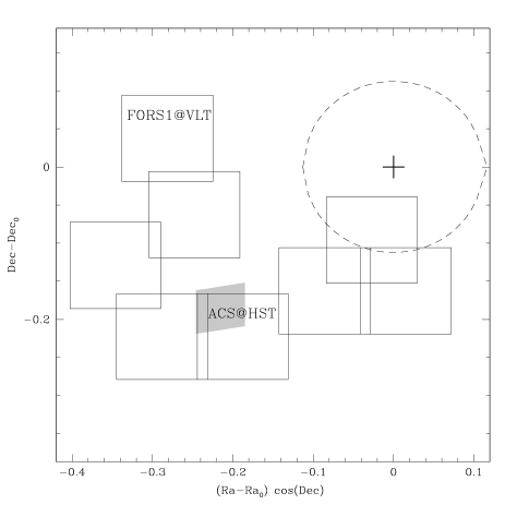
Figure 1: Map of the region sampled by the FORS1 observations. North is up, East on the right. The eight fields observed with FORS1 are shown. The grey box indicates the position of the ACS field. The cluster center and half-mass radius are indicated by the black cross and the dashed line, respectively.

Figure 2: FORS1 (R, B-R; left $panel$) and ACS ($I_{F814W},V_{F606W}-I_{F814W}$; right $panel$) CMDs of $\omega$ Cen.

3 Luminosity Function

To compute the LF of $\omega$ Cen we followed the procedure described below. As a first step, we computed the MS ridge line by averaging the colors of stars in the CMD over 0.2 mag boxes and applying a 2$\sigma$ clipping algorithm. Then, the LF has been computed by counting the number of objects in 0.5 mag wide bins separated by 0.1 mag along the R and $I_{F814W}$ axes. Only stars within $\pm 2.5$ times the color standard deviation around the MS ridge line have been considered (see De Marchi & Paresce 1995).

$\omega$ Cen is well known to harbour stellar populations with different metallicity (Norris, Freeman & Mighell 1996 and references therein) and, possibly, helium content (Norris 2004). The CMDs shown in Fig. 2 do not allow one to distinguish the different MS components of the cluster (except for the bMS population), making impossible to disentangle the contribution of each population to the LF. However, the metal-poor population of $\omega$ Cen comprises more than 70% of the entire cluster content (Pancino et al. 2000), thus dominating the shape of the LF. To check the validity of this assumption, we measured the LF of MS stars by excluding bMS stars in the magnitude range where this sequence is clearly distinguishable from the dominant cluster population. For this purpose, we considered bMS stars all the objects lying at a distance between 0.5 and 2.5 times the color standard deviation around the cluster ridge line on the blue side of the dominant cluster MS in the magnitude range $19.2<R<20.7$ and $19.2<I_{F814W}<20.9$ for the FORS1 and ACS sample, respectively. We found a constant difference between the LF measured with and without bMS stars over the entire magnitude range under investigation in both photometric samples. In particular, in both samples the deviations from the constant difference lie within $\Delta log~{}N<0.03$ over the entire magnitude range considered here (see Fig. 3). This indicates that although bMS stars constitute a significant fraction of the cluster population ($\sim$ 24%, Sollima et al. 2007), their presence does not significantly distort the shape of the measured LF. For this reason, in the following we will measure the LF of the global MS population assuming it as representative of the dominant cluster population.

The LF has been calculated by taking into account two important effects: (i) the photometric incompleteness and (ii) the contamination from field stars. In the following sections the adopted techniques to correct for these effects are described.

Figure 3: Difference between the LFs calculated with and without bMS stars for the FORS1 (upper $panel$) and the ACS (lower $panel$) sample. The average constant trend is indicated as a dashed line in both $panels$.

3.1 Photometry Incompleteness

A reliable determination of the LF from the CMDs of Fig. 2 requires the assessment of the degree of photometric incompleteness as a function of magnitude and color. For each individual field, the adopted procedure for artificial star experiments has been performed as follows (see Bellazzini et al. 2002):

• The magnitude of artificial stars was randomly extracted from a LF modeled to reproduce the observed LF for bright stars ($R<22$; $I_{F814W}<22$) and to provide large numbers of faint stars down to below the detection limits of our observations ($R\sim 24$; $I_{F814W}\sim 25$). The color of each star was obtained by deriving, for each extracted R and $I_{F814W}$ magnitude, the corresponding B and $V_{F606W}$ magnitude, for the two datasets respectively, by interpolating on the cluster ridge line. Thus, all the artificial stars lie on the cluster ridge line in the CMD;

• We divided the frames into grids of cells of known width (30 pixels) and randomly positioned only one artificial star per cell for each run;

• For the FORS1 sample, artificial stars were simulated with the DoPhot (Schechter et al. 1993) model for the fit, including any spatial variation of the shape of the PSF. For the ACS sample, artificial stars were simulated as gaussians with a $FWHM=0.1"$. Artificial stars were added on the original frames including Poisson photon noise. Each star was added to both B and R (F606W and F814W for the ACS sample) frames. The measurement process was repeated adopting the same procedure of the original measures and applying the same selection criteria described in Sollima et al. (2007) and in Sect. 2;

• The results of each single set of simulations were appended to a file until the desired total number of artificial stars was reached. The final result for each sub-field is a list containing the input and output values of positions and magnitudes.

More than 100,000 artificial stars have been produced providing a robust estimate of the photometric completeness over the entire magnitude extension of the MS. Fig. 4 shows the completeness factor ($\phi$) as a function of the R magnitude at three different distances from the cluster center for the FORS1 sample and as a function of the $I_{F}814W$ magnitude for the ACS sample. Only stars lying in the magnitude ranges where $\phi>0.5$ were used to construct the LF.

Figure 4: Completeness factor $\phi$ as a function of R magnitude at three different distances from the cluster center for the FORS1 sample (top three $panels$) and as a function of $I_{F814W}$ magnitude for the ACS sample (bottom $panel$).

3.2 Field Contamination

The contamination due to field stars was taken into account by using the Galaxy model of Robin et al. (2003). A synthetic catalog covering an area of 0.5 square degrees in the cluster direction has been retrieved. A sub-sample of stars has been randomly extracted from the entire catalog scaled to the ACS and FORS1 field of view. For the ACS sample, the V and I Johnson-Cousin magnitudes were converted into the ACS photometric system with the transformations of Sirianni et al. (2005). The number of stars contained in each magnitude bin within the color window used to measure the LF (see above) has been subtracted from the completeness-corrected MS star counts. The density of field objects in each magnitude bin is rather low (of the order of $<$2%), in agreement with theoretical expectations (Méndez & Van Altena 1996).

3.3 Results

Fig. 5 shows the R band LF of $\omega$ Cen calculated using stars lying in annuli of 4’ width at different distances from the cluster center. Note that the $\phi=0.5$ limit is reached at brighter magnitudes as inner (more crowded) regions are considered. As can be seen, in the magnitude range covered in this analysis, no significant variations are visible in the shape of the LFs calculated between 12’ and 20’ . This evidence provides further support to the hypothesis that this cluster is not affected by mass segregation. This result is in agreement with the findings of Anderson (1997) who compared the observed LF of $\omega$ Cen with the LF predicted by theoretical models with and without equipartition. Strong evidence of the lack of equipartition in $\omega$ Cen has been provided by Ferraro et al. (2006) on the basis of the comparison between the radial distribution of the blue straggler stars with that of the normal less massive cluster stars. As a consequence, the LF measured here can be used to derive a MF which can be considered a good approximation of the cluster IMF.

The F814W LF calculated for the external ACS field is shown in Fig. 6 and listed in Table 2. The LF reaches a peak at $I_{F814W}\sim$22.2 and clearly drops at fainter magnitudes, well before photometric incompleteness becomes significant. The LF of $\omega$ Cen measured by Richer et al. (1991), Elson et al. (1995), Anderson (1997) and De Marchi (1999) are overplotted to our data in Fig. 6. The original magnitudes provided by these authors have been converted into the ACS F814W magnitude with the transformations by Sirianni et al. (2005). All LFs showed in Fig. 6 have been normalized to have the same number of stars in the magnitude range $20<I_{F814W}<22$ . We note that the LF obtained in the present analysis extends to fainter magnitudes than those by Richer et al. (1991) and Elson et al. (1995), having a deepness comparable with those of De Marchi (1999) and Anderson (1997). Our ACS LF is in good agreement with that of Elson et al. (1995) and Anderson (1997). The LF by Richer et al. (1991) shows a steeper slope and continues to rise below $I_{F814W}>22.5$, at odds with the other LFs. This discrepancy is likely to be due to uncertainties in the number counts and completeness corrections at the faint end of the LF by Richer et al. (1991) whose observations were obtained from ground-based observations where crowding effects can produce severe incompleteness. The LF by De Marchi (1999) shows a drop for $I_{F814W}>22.5$ that is much more sudden than in our LF. However, the photometric dataset used by De Marchi (1999) has a limiting magnitude $\sim 1~{}mag$ brighter than that reached by our observations and is four times less populous than the ACS sample. For these reasons, we consider our LF more reliable at least at its faint end.

Table 2: LF of $\omega$ Cen measured in the ACS field

$I_{F814W}$	$N_{obs}$	$N_{field}$	$\phi$	N
19.0	183	4	0.980	183.7
19.1	190	6	0.980	190.9
19.2	194	7	0.980	195.0
19.3	202	7	0.980	202.1
19.4	202	5	0.980	202.1
19.5	170	3	0.980	172.5
19.6	191	3	0.980	191.9
19.7	189	3	0.980	189.9
19.8	194	2	0.980	194.0
19.9	192	2	0.980	193.9
20.0	187	3	0.980	186.8
20.1	180	1	0.980	180.7
20.2	212	5	0.980	212.3
20.3	234	5	0.980	234.8
20.4	242	5	0.980	241.9
20.5	251	5	0.980	252.1
20.6	268	4	0.980	264.5
20.7	269	3	0.980	263.5
20.8	255	4	0.980	250.2
20.9	268	7	0.980	265.5
21.0	284	6	0.980	281.8
21.1	287	7	0.980	287.9
21.2	298	8	0.980	300.1
21.3	307	6	0.980	309.3
21.4	322	6	0.980	324.7
21.5	319	5	0.979	321.7
21.6	354	5	0.979	356.5
21.7	408	5	0.979	408.8
21.8	458	8	0.979	459.0
21.9	503	8	0.979	505.2
22.0	494	7	0.978	499.3
22.1	530	4	0.977	536.4
22.2	541	5	0.976	550.1
22.3	538	9	0.976	545.5
22.4	536	9	0.974	545.0
22.5	542	11	0.973	553.9
22.6	532	11	0.971	544.7
22.7	492	12	0.969	504.7
22.8	506	10	0.967	517.3
22.9	487	8	0.964	500.1
23.0	483	6	0.961	494.8
23.1	494	13	0.957	510.3
23.2	465	11	0.952	485.5
23.3	439	8	0.946	459.9
23.4	426	9	0.940	444.3
23.5	385	13	0.932	405.2
23.6	361	9	0.923	383.9
23.7	366	7	0.912	388.2
23.8	350	6	0.901	379.3
23.9	324	5	0.889	357.5
24.0	316	6	0.875	354.0
24.1	310	5	0.860	351.5
24.2	289	9	0.841	335.5
24.3	241	6	0.818	287.5
24.4	239	8	0.783	298.2
24.5	194	5	0.724	263.9

Figure 5: R LF of $\omega$ Cen calculated between 12’ and 20’ from the cluster center. Each LF has been arbitrarily shifted of 0.15 in the y direction for clearity. The LF measured at 20’ is indicated for comparison with dashed lines.

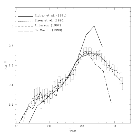
Figure 6: F814W LF of $\omega$ Cen calculated from the ACS external field (grey points). LFs by Richer et al. (1991, solid line), Elson et al. (1995, dotted line), Anderson (1997, short dashed line) and De Marchi (1999, long dashed line) are overplotted.

4 Comparison with GGC

In Fig. 7 we compare the deep MS-LF of $\omega$ Cen (obtained through the F814W filter) with those calculated by Piotto & Zoccali (1999) and Piotto, Cool & King (1997) for four other Galactic GCs, namely M15, M22, M55 and NGC 6397.

To compare the five LFs we assumed the distance and reddening scale described in Sollima et al. (2006), the extinction coefficient $A_{F814W}=1.825~{}E(B-V)$ and the photometric conversions by Sirianni et al. (2005). All of the LFs have been normalized to have the same number of stars in the magnitude range $19<I_{F814W}<20$ .

The LF of $\omega$ Cen has a slope similar to those of M22 and M55, being located between the two extreme cases of M15 and NGC 6397. In particular, M15 shows a significant overabundance of faint stars, incompatible with the measurement errors. A similar behaviour is observable also in GCs like M30 and M92 which have a MS-LF similar to that of M15 (see Piotto & Zoccali 1999).

Note that Piotto & Zoccali (1999) measured the LFs close to the cluster half-mass radius, where mass segregation effects are expected to be less severe.

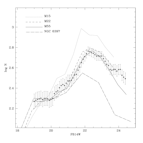
Figure 7: Comparison between the F814W LF of $\omega$ Cen (grey points) and the LFs of M15 (dotted line), NGC 6397 (dot-dashed line), M22 (dashed line) and M55 (solid line).

5 Mass Function

The LFs shown in Fig. 5 and 6 have been converted to MF using the mass-luminosity relation provided by Baraffe et al. (1997). To convert colors and magnitudes in the absolute system we adopted the distance modulus $(m-M)_{0}=13.72$ (Sollima et al. 2006), the reddening $E(B-V)=0.11$ (Lub 2001) and the extinction coefficients $A_{R}=2.35~{}E(B-V)$ (Savage & Mathis 1979) and $A_{F814W}=1.825~{}E(B-V)$ (Sirianni et al. 2005). Considering the negligible effects of dynamical evolution, the averaged LF of the FORS1 sample has been calculated using all the stars located at distances $r>12^{\prime}$ from the cluster center. In Fig. 8 the calculated MFs are shown. The two MFs have been normalized to have the same number of stars in the mass range $0.35M_{\odot}<M<0.65M_{\odot}$ . As can be noted, the obtained MFs agree quite well in the overlap region. The MF shown in Fig. 8 presents a well defined broken power-law shape, with a slope $\alpha\sim-2.3$ for masses $M>0.5M_{\odot}$ and a shallower slope ($\alpha\sim-0.8$) for smaller masses. A similar behaviour of the MF has been found by Reid & Gizis (1997) from the analysis of a sample of Galactic disk stars.

In principle, two effects can distort the obtained MF:

• The presence of a significant spread in the metal and possibly helium content (Norris et al. 1996; Norris 2004) that causes significant changes in the mass-luminosity relation. However, as shown in §3, the shape of the LF is dominated by the metal-poor population of $\omega$ Cen. For this reason we consider the MF derived here as representative of the dominant cluster population.

• Unresolved binary systems are shifted in the CMD toward brighter magnitudes and therefore can distort the derived MF.

To quantify the impact of a significant binary fraction in the shape of the derived MF, we performed a number of CMD simulation with different binary frequencies following the prescription of Bellazzini et al. (2002). The binary population has been simulated by extracting random pairs of stars from a broken power-low MF with given indices $\alpha_{1}$ and $\alpha_{2}$. The F814W and F606W fluxes of the binary components have been derived using the mass-luminosity relation of Baraffe et al. (1997) and summed in order to obtain the magnitudes of the unresolved binary system. Field stars were added following the procedure described in §3.2. In Fig. 9 the observed ACS CMD and the synthetic CMD simulated with a fraction of binaries $f_{b}=15\%$ are shown. As expected, a significant number of binary systems populate the synthetic CMD in a region located redward with respect to the dominant cluster MS (binary region). The comparison of the observed CMD with simulations accounting for a wide range of binary fractions indicates that the binary fraction in $\omega$ Cen must be smaller than $f_{b}<15\%$. Note that at least part of the stars populating the binary region in the observed ACS CMD could be single stars belonging to the metal-rich populations of $\omega$ Cen, that are not considered in the simulated CMD. For this reason, the binary fraction estimated above represents an upper limit to the true binary fraction in this stellar system. Then, we derived the LF of the simulated CMD adopting the same procedure described in the previous sections in order to quantify the effect of the presence of binary systems. We found that a broken power-low MF with indices $\alpha_{1}=-2.3$ (for $M>0.5~{}M_{\odot}$) and $\alpha_{2}=-0.8$ (for $M<0.5~{}M_{\odot}$) reproduces well the observed LF even assuming a binary fraction of $f_{b}=15\%$. Therefore, we conclude that binary stars have only a negligible effect on the shape of the MF in the considered mass range.

Some of the analytical IMF listed in Table 1 and the present-day MF derived by De Marchi et al. (2005) for a sample of Galactic GCs are overplotted to the MFs obtained in this paper in Fig. 10 . All MFs have been normalized in the mass range $0.5M_{\odot}<M<0.8M_{\odot}$ . While for masses $M<0.5M_{\odot}$ all the analytical IMFs reproduce quite well the observed MF of $\omega$ Cen, at lower masses the MF of $\omega$ Cen shows a stronger change of slope than those predicted by the analytical IMFs. In the low-mass range, the MF by De Marchi et al. (2005) predicts a deficiency of stars with respect to the MF measured in $\omega$ Cen, as expected in relaxed systems where low-mass stars are lost via evaporation and tidal interaction with the Milky Way.

Figure 8: Mass Function of $\omega$ Cen calculated from the FORS1 sample at distances $>$12’ from the cluster center (open points) and from the ACS external field (black points). A broken power-law with indices $\alpha_{1}=-2.3$ (for $M>0.5~{}M_{\odot}$) and $\alpha_{2}=-0.85$ (for $M<0.5~{}M_{\odot}$) is overplotted.

Figure 9: Observed ACS CMD (left $panel$) and simulated CMD with a binary fraction $f_{b}=0.15$ (right $panel$) in the magnitude range $18.5<I_{F814W}<21.5$.

Figure 10: Same as Fig. 8. The analytical relation by Salpeter (1955, solid line), De Marchi et al. (2005, dotted line) and Kroupa (2002, dashed line) are overplotted.

6 Discussion

In Sect. 3.3 we have shown that the MS-LF measured at different distances from the center does not show significant modifications, confirming that $\omega$ Cen is still dynamically young. This result is in agreement with that found by Anderson (1997) by comparing the observed MS-LF of $\omega$ Cen with the theoretical predictions with and without equipartition and by Ferraro et al. (2006) on the basis of the comparison between the radial distribution of the blue straggler stars and normal less massive cluster stars. Hence the observed MS-LF (and the derived MF) is expected to be essentially unaffected by internal dynamical processes (as e.g. mass segregation). Note that the fact that the MF slope derived for $\omega$ Cen is formally equal to that measured by Reid & Gizis (1997) for disk stars in the solar neighborhood fully supports this hypothesis.

A number of works suggests that $\omega$ Cen could be the remnant nucleus of a dwarf galaxy which merged in the past with the Milky Way (see Romano et al. 2007 and references therein). In this picture, the cluster experienced strong tidal losses during its interaction with the Galaxy. N-body simulations by Tsuchiya et al. (2004) suggest that the system lost $\sim$ 90% of its initial mass during the first 2 Gyr. Evidence that seems to confirm this hypothesis comes from the detection of a significant stellar overdensity resembling a pair of tidal tails surrounding $\omega$ Cen (Leon et al. 2000). However, this result has been questioned by Law et al. (2003) who found that Leon’s et al. tidal tails were strongly correlated with inhomogeneities in the reddening distribution. Note however that the lack of equipartition in $\omega$ Cen should lead the system to lose stars independently on their masses. Therefore, even strong stellar losses should not significantly distort the MS-LF of the cluster. Hence, the MS-LF shown in Fig. 6 should reflect the global primordial luminosity distribution of MS stars in the cluster.

If this consideration is true, the comparison of the MS-LF shown in Figure 7 casts some doubts on the ”universality” of the IMF. In fact, under the assumption that all stellar systems formed their stars following a ”universal” IMF, we would expect to observe a general agreement in the MS-LF shape (with respect to that measured in $\omega$ Cen) in poorly dynamically evolved clusters or a deficiency of faint (low-mass) stars in highly evolved clusters where dynamical effects have played a significant role. However in no cases we would expect to see an excess of low-mass stars.

Indeed, as shown in Figure 7, the MS-LF of $\omega$ Cen seems to share the same shape as that observed in M22 and M55, but significant differences in the low-luminosity star content are apparent with respect to M15 and NGC6397. In particular, while the overabundance of faint stars with respect to NGC6397 can be interpreted in terms of systematic evaporation of low-mass stars in the highly evolved cluster NGC6397, the difference with respect to M15 is much more puzzling. Indeed, if the LF in $\omega$ Cen reflects the primordial LF of the cluster, the difference with respect to M15 could be interpreted only in terms of a ”real” difference in the IMF. It is worth of noticing that other two clusters in the Piotto & Zoccali (1999) sample (M30 and M92) share the same behaviour of M15, showing a significant overabundance of faint low-mass stars with respect to $\omega$ Cen. The slopes of the low-mass end of the MF derived in these clusters by Piotto & Zoccali (1999) ($\alpha=-1.1,-1.2~{}\mbox{and}~{}-0.9$ for M15, M30 and M92, respectively) turn out to be smaller than that measured in this paper for $\omega$ Cen ($\alpha=-0.8$). Interestingly enough, all of these clusters have a metallicity significantly lower ($[Fe/H]\sim-2$) than the mean metallicity of $\omega$ Cen ($[Fe/H]\sim-1.7$, Suntzeff & Kraft 1996).

This evidence might suggest that a ”primordial” difference in the IMF of stellar systems as a function of the metallicity (i.e. metal poor clusters tend to produce more low-mass stars) could exist. The physical reason for this might be found in the higher efficiency of the fragmentation process in low-metallicity proto-cluster clouds (see Silk 1977). A possible dependence of the slope of the faint end of the clusters MFs on metallicity was also discussed and not excluded by Piotto & Zoccali (1999). Note that a similar result was also presented by McClure et al. (1986) and Djorgovski, Piotto & Capaccioli (1993) from the analysis of the LF of several Galactic GCs.

Clearly a deeper investigation is required to finally address this important question. However, the evidence presented here supports the possibility that the MF measured in $\omega$ Cen could be a reasonable approximation of the cluster IMF and that a variation of the IMF slope with the cluster metallicity could exist.

References

- Anderson (1997) Anderson, J., 1997, Ph.D. Thesis, University of California, Berkeley
- Baraffe et al. (1997) Baraffe I., Chabrier G., Allard F., Hauschildt P. H., 1997, A&A, 327, 1054
- Baraffe et al. (1996) Baraffe I., Chabrier G., 1996, ApJ, 461, L51
- Bedin et al. (2004) Bedin L. R., Piotto G., Anderson J., Cassisi S., King I. R., Momany Y., Carraro G., 2004, ApJ, 605, L125
- Bellazzini et al. (2002) Bellazzini M., Fusi Pecci F., Messineo M., Monaco L., Rood R. T., 2002, AJ, 123, 509
- Bertin et al. (1996) Bertin E., Arnouts S., 1996, A&AS, 117, 393
- Chabrier (2001) Chabrier G., 2001, ApJ, 554, 1274
- De Marchi & Paresce (1995) De Marchi G., Paresce F., 1995, A&A, 304, 202
- De Marchi (1999) De Marchi G., 1999, AJ, 117, 303
- De Marchi et al. (2005) De Marchi G., Paresce F., Portegies Zwart S., 2005, in ”The Initial Mass Function 50 years later”, ed. by E. Corbelli and F. Palle, Springer Dordrecht, 327, 77
- Djorgovski et al. (1993) Djorgovski S., Piotto G., Capaccioli M., 1993, AJ, 105, 6
- Elson et al. (1995) Elson R. A. W., Gilmore G. F., Santiago B. X., Casertano S., 1995, AJ, 110, 682
- Ferraro et al. (2006) Ferraro F. R., Sollima A., Rood R. T., Origlia L., Pancino E., Bellazzini M., 2006, ApJ, 638, 433
- Kroupa (2002) Kroupa P., 2002, Sci, 295, 82
- Larson (1998) Larson R. B., 1998, MNRAS, 301, 569
- Law et al. (2003) Law D. R., Majewski S. R., Skrutskie M. F., Carpenter J. M., Ayub H. F., 2003, AJ, 126, 1871
- Leon et al. (2000) Leon S., Meylan G., Combes F., 2000, A&A, 359, 907
- Lub (2002) Lub, J. 2002, in ”A Unique Window into Astrophysics”, ed. F. van Leeuwen, J. D. Hughes, & G.Piotto, ASP Conf.Series, 265, 95
- McClure et al. (1986) McClure R. et al., 1986, ApJ, 307, L49
- Mendez et al. (1996) Mendez R., van Altena W., 1996, AJ, 112, 655
- Miller et al. (1979) Miller G. E., Scalo J. M., 1979, ApJS, 41, 513
- Norris et al. (1996) Norris J. E., Freeman K. C., Mighell K. J., 1996, ApJ, 462, 241
- Norris (2004) Norris J. E., 2004, ApJ, 612, L25
- Pancino et al. (2000) Pancino E., Ferraro F. R., Bellazzini M., Piotto G., Zoccali M., 2000, ApJ, 534, L83
- Piotto et al. (1997) Piotto G., Cool A. M., King I. R., 1997, AJ, 113, 1345
- Piotto et al. (1999) Piotto G., Zoccali M., 1999, A&A, 345, 485
- Reid et al. (1997) Reid I. N., Gizis J. E., 1997, AJ, 113, 2246
- Richer et al. (1991) Richer H. B., Fahlman G. G., Buonanno R., Fusi Pecci F., Searle L., Thompson I. B., 1991, ApJ, 381, 147
- Romano et al. (2007) Romano D., Matteucci F., Tosi M., Pancino E., Bellazzini M., Ferraro F. R., Limongi M., Sollima A., 2007, MNRAS, 376, 405
- Salpeter (1955) Salpeter E. E., 1955, ApJ, 121, 161
- Savage & Mathis (1979) Savage B. D., Mathis J. S., 1979, ARA&A, 17, 73
- Schechter et al. (1993) Schechter P. L., Mateo M., Saha A., 1993, PASP, 105, 1342
- Silk (1977) Silk J., 1977, ApJ, 214, 718
- Sirianni et al. (2005) Sirianni et al., 2005, PASP, 117, 1049
- Sollima et al. (2006) Sollima A., Cacciari C., Valenti E., 2006, MNRAS, 372, 1675
- Sollima et al. (2007) Sollima A., Ferraro F. R., Bellazzini M., Origlia L., Straniero O., Pancino E., 2007, ApJ, 654, 915
- Suntzeff & Kraft (1996) Suntzeff N. B., Kraft R. P., 1996, AJ, 111, 1913
- Tsuchiya et al. (2004) Tsuchiya T., Korchagin V. I., Dinescu, D. I., 2004, MNRAS, 350, 1141
- van de Ven et al. (2006) van de Ven G., van den Bosch R. C. E., Verolme E. K., de Zeeuw P. T., 2006, A&A, 445, 513