Hopf Bifurcation in a Model for
Biological Control

Luis Fernando Mello
Instituto de Ciências Exatas, Universidade Federal de Itajubá
Avenida BPS 1303, Pinheirinho, CEP 37.500-903, Itajubá, MG, Brazil
e–mail: lfmelo@unifei.edu.br

Danilo Braun Santos
Centro de Ciências Sociais e Aplicadas, Universidade Mackenzie
Rua Itambé, 45, Consolação, CEP 01302-907, São Paulo, SP, Brazil
e–mail: danilobraun@mackenzie.com.br

Denis de Carvalho Braga
Instituto de Sistemas Elétricos e Energia, Universidade Federal de Itajubá
Avenida BPS 1303, Pinheirinho, CEP 37.500-903, Itajubá, MG, Brazil
e–mail: braga@unifei.edu.br

Abstract

In this paper we study the Lyapunov stability and Hopf bifurcation in a biological system which models the biological control of parasites of orange plantations.

Key-words: Hopf bifurcation, stability, periodic orbit, biological control.

MSC: 70K50, 70K20.

1 Introduction of the Mathematical Model

In this work we study a system of four coupled differential equations (1) which models the interaction between two biological species, each presenting two stages in their metamorphosis, living in a common habitat with limited resources.

The differential equations analyzed here are

$$P^{\prime} = \frac{dP}{dt}=\phi_{1}\left(1-\frac{M}{c_{1}}\right)M-(\alpha_{1}+\beta_{1})P-k_{1}PG$$

$$M^{\prime} = \frac{dM}{dt}=\alpha_{1}P-\mu_{1}M$$ (1)

$$L^{\prime} = \frac{dL}{dt}=\phi_{2}\left(1-\frac{G}{c_{2}}\right)G-(\alpha_{2}+\beta_{2})L+k_{2}PG$$

$$G^{\prime} = \frac{dG}{dt}=\alpha_{2}L-\mu_{2}G.$$

This model —an elaboration of Lotka-Volterra equations, taking into account the stages or compartments in the biological populations— was proposed by Yang and Ternes [1, 2] and Ternes [3] for a study of the biological control of orange plantations leaf parasites $P$, which is a pre-adult stage for $M$, by their natural enemies $L$, which is an early stage for $G$.

Other differential equations have been proposed as models for interacting populations partitioned in compartments, representing several situations of biological interest. See, among many others, Hethcote et al. [4], Jacquez and Simon [5] and Godfray and Waage [6].

In [1, 2] and [3] $P$ and $M$ are the densities of pupae and female adults of Phyllocnistis citrella (which in its larva stage is the citrus leafminer), $L$ and $G$ are the densities of larvae and female adults of its native parasitoid Galeopsomyia fausta (whose larvae feed on the pupae of $M$).

The meaning of the parameters in (1), where the notation of [1, 3] has been preserved, is as follows: $\alpha_{1}$ is the rate of pupae that give rise to adults $M$, $\beta_{1}$ is the mortality rate of pupae, $\mu_{1}$ is the mortality rate of adults $M$, $\phi_{1}$ is the rate of eggs that give rise to pupae, $c_{1}$ is the carrying capacity of the population $M$, $\alpha_{2}$ is the rate of larvae that, evolving through pupae, give rise to adults $G$, $\beta_{2}$ is the mortality rate of larvae and pupae, $\mu_{2}$ is the rate of mortality of adults $G$, $\phi_{2}$ is the oviposition rate of the parasite and $c_{2}$ is the carrying capacity of the population $G$. Here we assume that the pupa (respectively larva) population decreases (respectively increases) at a rate proportional to $P-G$ encounters that is $k_{1}PG$ (respectively $k_{2}PG$).

This model represents the evolution of female populations. If necessary the male populations can be estimated using the sexual ratio of each species.

Remark 1.1

All the parameters $\alpha_{1},\beta_{1},\mu_{1},\phi_{1},c_{1},k_{1},\alpha_{2},\beta_{2},\mu_{2},\phi_{2},c_{2},k_{2}$ are positive. As the damage to the $P$ population must be larger than the benefit to the $L$ population it is natural to assume that $k_{1}\geq k_{2}$.

Here will be established the location and the stability character of the equilibria of (1), four in number. Also is determined the bifurcation variety in the space of parameters, representing the transition from asymptotically stable to saddle type at the equilibrium point with positive coordinates, representing the coexistence of the two species. See Theorem 2.4 and its Corollary 2.5.

Fixing the all the parameters in (1) to biologically feasible values, taken from [3] and [7], but letting the interaction coefficients $k_{1}$ and $k_{2}$ vary in a positive quadrant, the nature of the bifurcation phenomenon in this plane by crossing the bifurcation curve is established. See Theorem 3.1 and Figure 1. This is done by means of a computer assisted calculation of the first Lyapunov coefficient, found to be positive. The Hopf bifurcation analysis of this point implies that the bifurcating periodic orbit is asymptotically unstable, of saddle type which surrounds an attracting equilibrium with small attracting basin. The dependence of the bifurcation curve on the parameter $c_{2}$ is studied in Theorem 3.3 and illustrated in Figure 3.

In Section 4 the implications of the results in this paper are discussed and interpreted from a wider perspective.

2 Stability Analysis of Equilibria

Assume the following notation:

$$R_{1}=\frac{\alpha_{1}\phi_{1}}{\mu_{1}(\alpha_{1}+\beta_{1})},\>\>R_{2}=\frac{\alpha_{2}\phi_{2}}{\mu_{2}(\alpha_{2}+\beta_{2})}.$$ (2)

The differential equations (1) have four equilibria

$$\mathcal{A}_{1}=(P_{1},M_{1},L_{1},G_{1})=(0,0,0,0),$$ (3)

$$\mathcal{A}_{2}=(P_{2},M_{2},L_{2},G_{2})=\left(\frac{c_{1}\mu_{1}}{\alpha_{1}}\left(1-\frac{1}{R_{1}}\right),c_{1}\left(1-\frac{1}{R_{1}}\right),0,0\right),$$ (4)

$$\mathcal{A}_{3}=(P_{3},M_{3},L_{3},G_{3})=\left(0,0,\frac{c_{2}\mu_{2}}{\alpha_{2}}\left(1-\frac{1}{R_{2}}\right),c_{2}\left(1-\frac{1}{R_{2}}\right)\right),$$ (5)

and

$$\mathcal{A}_{4}=(P_{4},M_{4},L_{4},G_{4}),$$ (6)

where

$$P_{4}=\frac{c_{1}\mu_{1}\phi_{2}}{\alpha_{1}^{2}\phi_{1}\phi_{2}+\mu_{1}^{2}c_{1}c_{2}k_{1}k_{2}}\left(\alpha_{1}\phi_{1}\left(1-\frac{1}{R_{1}}\right)-\mu_{1}c_{2}k_{1}\left(1-\frac{1}{R_{2}}\right)\right),$$

$$M_{4}=\frac{c_{1}\alpha_{1}\phi_{2}}{\alpha_{1}^{2}\phi_{1}\phi_{2}+\mu_{1}^{2}c_{1}c_{2}k_{1}k_{2}}\left(\alpha_{1}\phi_{1}\left(1-\frac{1}{R_{1}}\right)-\mu_{1}c_{2}k_{1}\left(1-\frac{1}{R_{2}}\right)\right),$$

$$L_{4}=\frac{c_{2}\mu_{2}\alpha_{1}\phi_{1}}{\alpha_{2}(\alpha_{1}^{2}\phi_{1}\phi_{2}+\mu_{1}^{2}c_{1}c_{2}k_{1}k_{2})}\left(c_{1}\mu_{1}k_{2}\left(1-\frac{1}{R_{1}}\right)+\alpha_{1}\phi_{2}\left(1-\frac{1}{R_{2}}\right)\right),$$

$$G_{4}=\frac{c_{2}\alpha_{1}\phi_{1}}{\alpha_{1}^{2}\phi_{1}\phi_{2}+\mu_{1}^{2}c_{1}c_{2}k_{1}k_{2}}\left(c_{1}\mu_{1}k_{2}\left(1-\frac{1}{R_{1}}\right)+\alpha_{1}\phi_{2}\left(1-\frac{1}{R_{2}}\right)\right).$$

Remark 2.1

If $R_{1}>1$ and $R_{2}>1$, then the equilibria $\mathcal{A}_{1}$, $\mathcal{A}_{2}$ and $\mathcal{A}_{3}$, have only non-negative coordinates. If $k_{1}<k_{1_{max}}$, where

$$k_{1_{max}}=\frac{\alpha_{1}\phi_{1}\left(1-\frac{1}{R_{1}}\right)}{c_{2}\mu_{1}\left(1-\frac{1}{R_{2}}\right)},$$ (7)

then the coordinates of the equilibrium $\mathcal{A}_{4}$ are also non-negative.

The Jacobian matrix of (1) at ${\bf x}=(P,M,L,G)\in\mathbb{R}^{4}$ has the form

$$J({\bf x})=\left(\begin{array}[]{cccc}-\alpha_{1}-\beta_{1}-k_{1}G&\phi_{1}-\frac{2\phi_{1}M}{c_{1}}&0&-k_{1}P\\ \alpha_{1}&-\mu_{1}&0&0\\ k_{2}G&0&-\alpha_{2}-\beta_{2}&\phi_{2}-\frac{2\phi_{2}G}{c_{2}}+k_{2}P\\ 0&0&\alpha_{2}&-\mu_{2}\end{array}\right),$$ (8)

while its characteristic polynomial is given by

$$p(\lambda)=det(J({\bf x})-\lambda I)=\Theta_{1}\>\Theta_{2}\\ +\alpha_{2}(\mu_{1}+\lambda)k_{1}k_{2}PG,$$ (9)

where

$$\Theta_{1}=(\mu_{1}+\lambda)(\alpha_{1}+\beta_{1}+k_{1}G+\lambda)-\alpha_{1}\left(\phi_{1}-\frac{2\phi_{1}M}{c_{1}}\right)$$

and

$$\Theta_{2}=(\mu_{2}+\lambda)(\alpha_{2}+\beta_{2}+\lambda)-\alpha_{2}\left(\phi_{2}-\frac{2\phi_{2}G}{c_{2}}+k_{2}P\right).$$

Recall that an equilibrium point ${\bf x_{0}}$ is said to be a saddle of type $n-p$ if the Jacobian matrix $J({\bf x_{0}})$ has $n$ eigenvalues with negative real parts and $p$ eigenvalues with positive real parts.

Theorem 2.2

If $R_{1}>1$, $R_{2}>1$ and $k_{1}<k_{1_{max}}$ then:

1. The equilibrium $\mathcal{A}_{1}$ is a saddle of type 2-2;

2. The equilibrium $\mathcal{A}_{2}$ is a saddle of type 3-1;

3. The equilibrium $\mathcal{A}_{3}$ is a saddle of type 3-1.

Proof. From (9) the eigenvalues of $J(\mathcal{A}_{1})$ are given by

$$\begin{array}[]{ll}\lambda_{1}=&-\frac{1}{2}(\alpha_{1}+\beta_{1}+\mu_{1})+\frac{1}{2}\sqrt{(\alpha_{1}+\beta_{1}+\mu_{1})^{2}+4\alpha_{1}\phi_{1}[1-\frac{1}{R_{1}}]},\\ \\ \lambda_{2}=&-\frac{1}{2}(\alpha_{1}+\beta_{1}+\mu_{1})-\frac{1}{2}\sqrt{(\alpha_{1}+\beta_{1}+\mu_{1})^{2}+4\alpha_{1}\phi_{1}[1-\frac{1}{R_{1}}]},\\ \\ \lambda_{3}=&-\frac{1}{2}(\alpha_{2}+\beta_{2}+\mu_{2})+\frac{1}{2}\sqrt{(\alpha_{2}+\beta_{2}+\mu_{2})^{2}+4\alpha_{2}\phi_{2}[1-\frac{1}{R_{2}}]},\\ \\ \lambda_{4}=&-\frac{1}{2}(\alpha_{2}+\beta_{2}+\mu_{2})-\frac{1}{2}\sqrt{(\alpha_{2}+\beta_{2}+\mu_{2})^{2}+4\alpha_{2}\phi_{2}[1-\frac{1}{R_{2}}]},\end{array}\\$$

and satisfy: $\lambda_{1}>0$, $\lambda_{2}<0$, $\lambda_{3}>0$ and $\lambda_{4}<0$. This proves the first assertion.

From (9) the eigenvalues of $J(\mathcal{A}_{2})$ are given by

$$\lambda_{1}=-\frac{1}{2}(\alpha_{1}+\beta_{1}+\mu_{1})+\frac{1}{2}\sqrt{(\alpha_{1}+\beta_{1}+\mu_{1})^{2}-4\alpha_{1}\phi_{1}[1-\frac{1}{R_{1}}]},$$

$$\lambda_{2}=-\frac{1}{2}(\alpha_{1}+\beta_{1}+\mu_{1})-\frac{1}{2}\sqrt{(\alpha_{1}+\beta_{1}+\mu_{1})^{2}-4\alpha_{1}\phi_{1}[1-\frac{1}{R_{1}}]},$$

$$\begin{array}[]{cl}\lambda_{3}=&-\frac{1}{2}(\alpha_{2}+\beta_{2}+\mu_{2})+\\ \\ &\frac{1}{2}\sqrt{(\alpha_{2}+\beta_{2}+\mu_{2})^{2}+4\alpha_{2}\phi_{2}[1-\frac{1}{R_{2}}]+4\frac{c_{1}\alpha_{2}\mu_{1}}{\alpha_{1}}[1-\frac{1}{R_{1}}]k_{2}},\end{array}$$

$$\begin{array}[]{cl}\lambda_{4}=&-\frac{1}{2}(\alpha_{2}+\beta_{2}+\mu_{2})-\\ \\ &\frac{1}{2}\sqrt{(\alpha_{2}+\beta_{2}+\mu_{2})^{2}+4\alpha_{2}\phi_{2}[1-\frac{1}{R_{2}}]+4\frac{c_{1}\alpha_{2}\mu_{1}}{\alpha_{1}}[1-\frac{1}{R_{1}}]k_{2}}.\end{array}$$

Is immediate to see that $\lambda_{3}>0$ and $\lambda_{4}<0$. If

$$\phi_{1}>\frac{1}{4\alpha_{1}}[(\alpha_{1}+\beta_{1}+\mu_{1})^{2}+4\mu_{1}(\alpha_{1}+\beta_{1})]$$

then $\lambda_{1}$ and $\lambda_{2}$ are complex with negative real parts and if

$$\phi_{1}\leq\frac{1}{4\alpha_{1}}[(\alpha_{1}+\beta_{1}+\mu_{1})^{2}+4\mu_{1}(\alpha_{1}+\beta_{1})]$$

then $\lambda_{1}<0$ and $\lambda_{2}<0$. This proves the second assertion.

From (9) the eigenvalues of $J(\mathcal{A}_{3})$ are given by

$$\begin{array}[]{cl}\lambda_{1}=&-\frac{1}{2}(\alpha_{1}+\beta_{1}+\mu_{1}+c_{2}k_{1}[1-\frac{1}{R_{2}}])+\\ \\ &\frac{1}{2}\sqrt{(\alpha_{1}+\beta_{1}-\mu_{1}+c_{2}k_{1}[1-\frac{1}{R_{2}}])^{2}+4\alpha_{1}\phi_{1}},\end{array}$$

$$\begin{array}[]{cl}\lambda_{2}=&-\frac{1}{2}(\alpha_{1}+\beta_{1}+\mu_{1}+c_{2}k_{1}[1-\frac{1}{R_{2}}])-\\ \\ &\frac{1}{2}\sqrt{(\alpha_{1}+\beta_{1}-\mu_{1}+c_{2}k_{1}[1-\frac{1}{R_{2}}])^{2}+4\alpha_{1}\phi_{1}},\end{array}$$

$$\lambda_{3}=-\frac{1}{2}(\alpha_{2}+\beta_{2}+\mu_{2})+\frac{1}{2}\sqrt{(\alpha_{2}+\beta_{2}+\mu_{2})^{2}-4\alpha_{2}\phi_{2}[1-\frac{1}{R_{2}}]},$$

$$\lambda_{4}=-\frac{1}{2}(\alpha_{2}+\beta_{2}+\mu_{2})-\frac{1}{2}\sqrt{(\alpha_{2}+\beta_{2}+\mu_{2})^{2}-4\alpha_{2}\phi_{2}[1-\frac{1}{R_{2}}]}.$$

It follows that $\lambda_{1}>0$, $\lambda_{2}<0$. If

$$\phi_{2}>\frac{1}{4\alpha_{2}}[(\alpha_{2}+\beta_{2}+\mu_{2})^{2}+4\mu_{2}(\alpha_{2}+\beta_{2})]$$

then $\lambda_{3}$ and $\lambda_{4}$ are complex with negative real parts and if

$$\phi_{2}\leq\frac{1}{4\alpha_{2}}[(\alpha_{2}+\beta_{2}+\mu_{2})^{2}+4\mu_{2}(\alpha_{2}+\beta_{2})]$$

then $\lambda_{3}<0$ and $\lambda_{4}<0$. This proves the last assertion.

$\blacksquare$

For the sake of completeness we state the following lemma which is a particular case of the Theorem of Routh–Hurwitz. See [8], p. 62.

Lemma 2.3

The polynomial $L(\lambda)=a_{0}\lambda^{4}+a_{1}\lambda^{3}+a_{2}\lambda^{2}+a_{3}\lambda+a_{4}$, $a_{0}>0$, with real coefficients has all roots with negative real parts if and only if the numbers $a_{1},a_{2},a_{3},a_{4}$ are positive and the inequality

$$\Delta=a_{1}\;a_{2}\;a_{3}-a_{0}\;a_{3}^{2}-a_{1}^{2}\;a_{4}>0$$

is satisfied.

Theorem 2.4

If $R_{1}>1$, $R_{2}>1$ and $k_{1}<k_{1_{max}}$ then all the coefficients of the characteristic polynomial of $J(\mathcal{A}_{4})$ are positive. Therefore, if

$$\Delta=a_{1}\;a_{2}\;a_{3}-a_{3}^{2}-a_{1}^{2}\;a_{4}>0,$$ (10)

where

$$a_{1}=\alpha_{1}+\beta_{1}+\mu_{1}+\alpha_{2}+\beta_{2}+\mu_{2}+k_{1}G_{4},$$

$$a_{2}=\frac{\alpha_{1}\phi_{1}}{c_{1}}M_{4}+\frac{\alpha_{2}\phi_{2}}{c_{2}}G_{4}+(\alpha_{1}+\beta_{1}+\mu_{1}+k_{1}G_{4})(\alpha_{2}+\beta_{2}+\mu_{2}),$$

$$a_{3}=(\alpha_{1}+\beta_{1}+\mu_{1}+k_{1}G_{4})\frac{\alpha_{2}\phi_{2}}{c_{2}}G_{4}+(\alpha_{2}+\beta_{2}+\mu_{2})\frac{\alpha_{1}\phi_{1}}{c_{1}}M_{4}+\alpha_{2}k_{1}k_{2}P_{4}G_{4},$$

$$a_{4}=\alpha_{2}\alpha_{1}\phi_{1}\left(k_{2}\left(1-\frac{1}{R_{1}}\right)P_{4}+\frac{\phi_{2}}{c_{1}}\left(1-\frac{1}{R_{2}}\right)M_{4}\right),$$

then the differential equations (1) have an asymptotically stable equilibrium point at $\mathcal{A}_{4}$. If

$$\Delta<0$$

then $\mathcal{A}_{4}$ is unstable.

Proof. From (9) the characteristic polynomial of $J(\mathcal{A}_{4})$ is given by

$$[\lambda^{2}+(\alpha_{1}+\beta_{1}+\mu_{1}+k_{1}G_{4})\lambda+\frac{\alpha_{1}\phi_{1}}{c_{1}}M_{4}][\lambda^{2}+(\alpha_{2}+\beta_{2}+\mu_{2})\lambda+\frac{\alpha_{2}\phi_{2}}{c_{2}}G_{4}]$$

$$+\alpha_{2}\mu_{1}k_{1}k_{2}P_{4}G_{4}+\alpha_{2}k_{1}k_{2}P_{4}G_{4}\lambda,$$

which can be written as

$$\begin{array}[]{l}\lambda^{4}+\lambda^{3}[\alpha_{1}+\beta_{1}+\mu_{1}+\alpha_{2}+\beta_{2}+\mu_{2}+k_{1}G_{4}]\\ \\ +\lambda^{2}[\frac{\alpha_{1}\phi_{1}}{c_{1}}M_{4}+\frac{\alpha_{2}\phi_{2}}{c_{2}}G_{4}+(\alpha_{1}+\beta_{1}+\mu_{1}+k_{1}G_{4})(\alpha_{2}+\beta_{2}+\mu_{2})]\\ \\ +\lambda[(\alpha_{1}+\beta_{1}+\mu_{1}+k_{1}G_{4})\frac{\alpha_{2}\phi_{2}}{c_{2}}G_{4}+(\alpha_{2}+\beta_{2}+\mu_{2})\frac{\alpha_{1}\phi_{1}}{c_{1}}M_{4}+\alpha_{2}k_{1}k_{2}P_{4}G_{4}]\\ \\ +\frac{\alpha_{1}\phi_{1}}{c_{1}}M_{4}\frac{\alpha_{2}\phi_{2}}{c_{2}}G_{4}+\alpha_{2}\mu_{1}k_{1}k_{2}P_{4}G_{4}.\end{array}$$

Now it is simple to see that the coefficients of the characteristic polynomial are given by $a_{1},a_{2},a_{3},a_{4}$ above. From the hypotheses these coefficients are positive. The stability at $\mathcal{A}_{4}$ follows from Lemma 2.3.

$\blacksquare$

The following corollary is immediate from the fact that $a_{i}>0$.

Corollary 2.5

The Jacobian matrix $J(\mathcal{A}_{4})$ has a pair of complex eigenvalues with zero real part if and only if

$$a_{3}^{2}-a_{1}\;a_{2}\;a_{3}+a_{1}^{2}\;a_{4}=0,$$ (11)

where $a_{i}$ are defined in Theorem 2.4.

In next section we study the stability of $\mathcal{A}_{4}$ under the condition (11), complementary to the range of validity of Theorem 2.4.

3 Hopf Bifurcation Analysis

3.1 Generalities on Hopf Bifurcations

The study outlined below is based on the approach found in the book of Kuznetsov [9], pp 175-178.

Consider the differential equations

$${\bf x}^{\prime}=f({\bf x},{\bf\mu}),$$ (12)

where ${\bf x}\in\mathbb{R}^{4}$ and ${\bf\mu}\in\mathbb{R}^{m}$ is a vector of control parameters. Suppose (12) has an equilibrium point ${\bf x}={\bf x_{0}}$ at ${\bf\mu}={\bf\mu_{0}}$ and represent

$$F({\bf x})=f({\bf x},{\bf\mu_{0}})$$ (13)

as

$$F({\bf x})=A{\bf x}+\frac{1}{2}\>B({\bf x},{\bf x})+\frac{1}{6}\>C({\bf x},{\bf x},{\bf x})+O(||{\bf x}||^{4}){},$$

where $A=f_{\bf x}(0,{\bf\mu_{0}})$ and

$$B_{i}({\bf x},{\bf y})=\sum_{j,k=1}^{4}\frac{\partial^{2}F_{i}(\xi)}{\partial\xi_{j}\>\partial\xi_{k}}\bigg{|}_{\xi=0}x_{j}\;y_{k},$$ (14)

$$C_{i}({\bf x},{\bf y},{\bf z})=\sum_{j,k,l=1}^{4}\frac{\partial^{3}F_{i}(\xi)}{\partial\xi_{j}\>\partial\xi_{k}\>\partial\xi_{l}}\bigg{|}_{\xi=0}x_{j}\;y_{k}\>z_{l},$$ (15)

for $i=1,2,3,4$. Here the variable ${\bf x}-{\bf x_{0}}$ is also denoted by ${\bf x}$.

Suppose $({\bf x_{0}},{\bf\mu_{0}})$ is an equilibrium point of (12) where the Jacobian matrix $A$ has a pair of purely imaginary eigenvalues $\lambda_{3,4}=\pm i\omega_{0}$, $\omega_{0}>0$, and no other critical (i.e., on the imaginary axis) eigenvalues.

Let $p,q\in\mathbb{C}^{4}$ be vectors such that

$$Aq=i\omega_{0}\>q,\>\>A^{\top}p=-i\omega_{0}\>p,\>\>\langle p,q\rangle=\sum_{i=1}^{4}\bar{p}_{i}\>q_{i}\>\>=1.$$ (16)

The two dimensional center manifold can be parameterized by $w\in\mathbb{R}^{2}=\mathbb{C}$, by means of ${\bf x}=H(w,\bar{w})$, which is written as

$$H(w,{\bar{w}})=wq+{\bar{w}}{\bar{q}}+\sum_{2\leq j+k\leq 3}\frac{1}{j!k!}\>h_{jk}w^{j}{\bar{w}}^{k}+O(|w|^{4}),$$

with $h_{jk}\in\mathbb{C}^{4}$, $h_{jk}={\bar{h}}_{kj}$.

Substituting these expressions into (12) and (3.1) one has

$$H_{w}(w,\bar{w})w^{\prime}+H_{\bar{w}}(w,\bar{w}){\bar{w}}^{\prime}=F(H(w,\bar{w})).$$ (17)

The complex vectors $h_{ij}$ are to be determined so that equation (17) writes as follows

$$w^{\prime}=i\omega_{0}w+\frac{1}{2}\>G_{21}w|w|^{2}+O(|w|^{4}),$$

with $G_{21}\in\mathbb{C}$.

Solving the linear system obtained by expanding (17), the coefficients of the quadratic terms of (13) lead to

$$h_{11}=-A^{-1}B(q,{\bar{q}}),$$ (18)

$$h_{20}=(2i\omega_{0}I_{4}-A)^{-1}B(q,q),$$ (19)

where $I_{4}$ is the unit $4\times 4$ matrix.

The coefficients of the cubic terms are also uniquely calculated, except for the term $w^{2}{\bar{w}}$, whose coefficient satisfies a singular system for $h_{21}$

$$(i\omega_{0}I_{4}-A)h_{21}=C(q,q,{\bar{q}})+B({\bar{q}},h_{20})+2B(q,h_{11})-G_{21}q,$$ (20)

which has a solution if and only if

$$\langle p,C(q,q,\bar{q})+B(\bar{q},h_{20})+2B(q,h_{11})-G_{21}q\rangle=0.$$

Therefore

$$G_{21}=\langle p,C(q,q,\bar{q})+B(\bar{q},(2i\omega_{0}I_{4}-A)^{-1}B(q,q))-2B(q,A^{-1}B(q,\bar{q}))\rangle,$$ (21)

and the first Lyapunov coefficient $l_{1}$ – which decides by the analysis of third order terms at the equilibrium its stability, if negative, or instability, if positive – is defined by

$$l_{1}=\frac{1}{2\;\omega_{0}}\>{\rm Re}\;G_{21}.$$ (22)

A Hopf point $({\bf x_{0}},{\bf\mu_{0}})$ is an equilibrium point of (12) where the Jacobian matrix $A$ has a pair of purely imaginary eigenvalues $\lambda_{3,4}=\pm i\omega_{0}$, $\omega_{0}>0$, and no other critical eigenvalues. At a Hopf point, a two dimensional center manifold is well-defined, which is invariant under the flow generated by (12) and can be smoothly continued to nearby parameter values.

A Hopf point is called transversal if the curves of complex eigenvalues cross the imaginary axis with non-zero derivative.

In a neighborhood of a transversal Hopf point with $l_{1}\neq 0$ the dynamic behavior of the system (12), reduced to the family of parameter-dependent continuations of the center manifold, is orbitally topologically equivalent to the complex normal form

$$w^{\prime}=(\gamma+i\omega)w+l_{1}w|w|^{2},$$ (23)

$w\in\mathbb{C}$, $\gamma$, $\omega$ and $l_{1}$ are smooth continuations of $0$, $\omega_{0}$ and the first Lyapunov coefficient at the Hopf point [9], respectively. When $l_{1}<0$ ($l_{1}>0$) a family of stable (unstable) periodic orbits can be found on this family of center manifolds, shrinking to the equilibrium point at the Hopf point.

3.2 Hopf Bifurcation in the Biological Model

In this subsection we analyze the stability at $\mathcal{A}_{4}$ given by (6) under the condition (11). From (12) write the Taylor expansion (3.1) of $f({\bf x})$. Thus

$$A=\left(\begin{array}[]{cccc}-(\alpha_{1}+\beta_{1})-k_{1}G_{4}&\phi_{1}(1-\frac{2M_{4}}{c_{1}})&0&-k_{1}P_{4}\\ \alpha_{1}&-\mu_{1}&0&0\\ k_{2}G_{4}&0&-(\alpha_{2}+\beta_{2})&\phi_{2}(1-\frac{2G_{4}}{c_{2}})+k_{2}P_{4}\\ 0&0&\alpha_{2}&-\mu_{2}\end{array}\right)$$ (24)

and, with the notation in (3.1) to (15), one has

$$F({\bf x})\,-\,A{\bf x}=\left(-\frac{\phi_{1}M^{2}}{c_{1}}-k_{1}PG,0,-\frac{\phi_{2}G^{2}}{c_{2}}+k_{2}PG,0\right).$$ (25)

From (3.1), (14), (15) and (25) one has

$$B({\bf x},{\bf y})=\left(B_{1}({\bf x},{\bf y}),0,B_{3}({\bf x},{\bf y}),0\right),$$ (26)

where

$$B_{1}({\bf x},{\bf y})=-\frac{2\phi_{1}}{c_{1}}\>x_{2}\;y_{2}-k_{1}(x_{1}\;y_{4}+x_{4}\;y_{1}),$$

$$B_{3}({\bf x},{\bf y})=-\frac{2\phi_{2}}{c_{2}}\>x_{4}\;y_{4}+k_{2}(x_{1}\;y_{4}+x_{4}\;y_{1}),$$

and

$$C({\bf x},{\bf y},{\bf z})\equiv 0.$$ (27)

To pursue the analysis consider the following table of specific parameters

$$\begin{array}[]{|lllll|}\hline\cr\alpha_{1}=0.7&\beta_{1}=0.003&\mu_{1}=0.6&\phi_{1}=2.3&c_{1}=400000\\ \alpha_{2}=0.3&\beta_{2}=0.0015&\mu_{2}=0.4&\phi_{2}=4&c_{2}=100\\ \hline\cr\end{array}$$ (28)

taken from [7] and [3], where their biological feasibility in Brazilian fields is discussed.

With the above parameter values the differential equations (1) are in fact a two parameter system of differential equations where the parameters are $k_{1}$ and $k_{2}$ and can be written equivalently as

$${\bf x}^{\prime}=f({\bf x},k_{1},k_{2}),$$ (29)

with $f({\bf x},k_{1},k_{2})$ defined by the right-hand sides of (1).

With the parameter values of table (28), the equilibrium point $\mathcal{A}_{4}$ (6) has the following coordinates

$$P_{4}=\frac{800000\;(1.425-64.764\;k_{1})}{4.508+1.444\cdot 10^{7}\;k_{1}\;k_{2}},\>M_{4}=\frac{933333.333\;(1.425-64.764\;k_{1})}{4.508+1.444\cdot 10^{7}\;k_{1}\;k_{2}},$$

$$L_{4}=\frac{444.444\;(1.216+85550.400\;k_{2})}{4.508+1.444\cdot 10^{7}\;k_{1}\;k_{2}},\>G_{4}=\frac{333.333\;(1.216+85550.400\;k_{2})}{4.508+1.444\cdot 10^{7}\;k_{1}\;k_{2}},$$

while $R_{1}$, $R_{2}$ and $k_{1_{max}}$, given by (2) and (7), have the form

$$R_{1}=3.81697,\>\>R_{2}=9.95025,\>\>k_{1_{max}}=0.0220159.$$ (30)

From the above equation and the Remark 1.1, the set of admissible parameters is given by (see Fig 1)

$$\mathcal{S}=\{(k_{1},k_{2})|\>0<k_{1}<k_{1_{max}}=0.0220159\>\>{\mbox{and}}\>\>0<k_{2}\leq k_{1}\}.$$ (31)

In this set $\mathcal{S}$ the curve $\Sigma=\Delta^{-1}(0)$ is well-defined (see (11)), where $\Delta$ is given by

$$1699.422-233762.372k_{1}-6.860\cdot 10^{7}k_{2}-1.114\cdot 10^{7}k_{1}^{2}-2.175\cdot 10^{12}k_{2}^{2}-$$

$$4.994\cdot 10^{10}k_{1}k_{2}-2.147\cdot 10^{8}k_{1}^{3}-4.079\cdot 10^{12}k_{1}^{2}k_{2}-1.529\cdot 10^{15}k_{1}k_{2}^{2}-$$

$$7.809\cdot 10^{13}k_{1}^{3}k_{2}-4.319\cdot 10^{17}k_{1}^{2}k_{2}^{2}-1.540\cdot 10^{19}k_{1}k_{2}^{3}-4.755\cdot 10^{14}k_{1}^{4}k_{2}-$$

$$1.752\cdot 10^{19}k_{1}^{3}k_{2}^{2}-6.741\cdot 10^{21}k_{1}^{2}k_{2}^{3}+2.940\cdot 10^{18}k_{1}^{4}k_{2}^{2}-1.703\cdot 10^{24}k_{1}^{3}k_{2}^{3}+$$

$$1.634\cdot 10^{26}k_{1}^{2}k_{2}^{4}+6.618\cdot 10^{24}k_{1}^{4}k_{2}^{3}-4.437\cdot 10^{28}k_{1}^{3}k_{2}^{4}+1.643\cdot 10^{29}k_{1}^{4}k_{2}^{4},$$

representing the parameters where $J(\mathcal{A}_{4})$ has a pair of purely imaginary eigenvalues $\lambda_{3,4}=\pm i\omega_{0}$ with

$$\omega_{0}=1.2909\Big{[}0.6909+\frac{0.0071(-2.6479\cdot 10^{-6}+k_{2})(1.4219\cdot 10^{-5}+k_{2})}{k_{2}(3.1305\cdot 10^{-7}+k_{1}k_{2})}+$$

$$\frac{8.5745\cdot 10^{-7}}{k_{2}}+\Big{(}\frac{1}{(6.2611\cdot 10^{-7}+k_{1}k_{2})k_{1}k_{2}}\Big{(}(1.0783\cdot 10^{-9}+$$ (32)

$$5.0825\cdot 10^{-5}k_{2})k_{2}-3.1286\cdot 10^{-4}(1.3649\cdot 10^{-3}k_{2})(6.0127\cdot 10^{-6}+k_{2})+$$

$$0.9391\;k_{1}^{2}(9.5980\cdot 10^{-8}+k_{2})(8.1563\cdot 10^{-6}+k_{2})\Big{)}\Big{)}^{1/2}\Big{]}^{1/2}.$$

Figure 1: Set of admissible parameters $\mathcal{S}$ and Hopf curve $\Sigma$.

Thus one has (see Fig. 1)

$$\mathcal{S}=\mathcal{S}_{+}\cup\Sigma\cup\mathcal{S}_{-}.$$

For parameter values in the region $\mathcal{S}_{+}$ the equilibrium $\mathcal{A}_{4}$ is unstable since the Jacobian matrix $J(\mathcal{A}_{4})$ has two complex eigenvalues with positive real parts and two other real negative eigenvalues. For parameter values in the region $\mathcal{S}_{-}$ the equilibrium $\mathcal{A}_{4}$ is asymptotically stable since $J(\mathcal{A}_{4})$ has two complex eigenvalues with negative real parts and two other real negative eigenvalues. The curve $\Sigma$ is the curve of admissible parameters where the equilibrium $\mathcal{A}_{4}$ is a Hopf point.

Theorem 3.1

Consider the differential equations (1) with the parameters given in the table (28). If $(k_{1},k_{2})\in\Sigma$ then the two parameter family of differential equations (1) has a transversal Hopf point at $\mathcal{A}_{4}$. This Hopf point at $\mathcal{A}_{4}$ is unstable and for each $(k_{1},k_{2})\in\mathcal{S}_{-}$, but close to $\Sigma$, there exists an unstable periodic orbit near the asymptotically stable equilibrium point $\mathcal{A}_{4}$. See Fig 1.

Computer Assisted Proof. The proof follows the steps outlined in Subsection 3.1. However, all the expressions in the proof are too long to be put in print. For this reason, in the site [10] have been posted the main steps of the long calculations involved in the proof. This has been done in the form of a notebook for MATHEMATICA 5 [11]. A sufficient condition for being a Hopf point is that the first Lyapunov coefficient $l_{1}\neq 0$. In fact, it can be shown numerically that $l_{1}(k_{1},k_{2})>0$ for all values $(k_{1},k_{2})\in\Sigma$. A particular case and other related calculations are considered below for the sake of illustration.

Take the particular point $Q=(k_{1}=0.00331,k_{2}=0.00100)\in\Sigma$ with five decimal round-off coordinates [7]. For these values of the parameters

$$\mathcal{A}_{4}=(18543.57758,21634.17385,738.0525862,553.5394397).$$

The Jacobian matrix $J(\mathcal{A}_{4})$ has eigenvalues

$$\lambda_{1}=-3.61058,\>\lambda_{2}=-0.22912,\>\lambda_{3,4}=\pm 2.84670i,$$

and thus

$$\omega_{0}=2.84670.$$ (33)

From (16) the eigenvectors $q$ and $p$ have the form

$$q=\left(\begin{array}[]{c}820.5542609+1080.774610i\\ 295.1756045-139.5588184i\\ 862.8021803+130.4940530i\\ 26.01486634-87.27100717i\end{array}\right),$$

$$p=\left(\begin{array}[]{c}0.00003314748646+0.00006274424412i\\ -0.00003846764141+0.00003199241887i\\ 0.0005233172006+0.00007678211168i\\ 0.001254520214-0.004888597529i\end{array}\right).$$

One has

$$B(q,q)=\left(\begin{array}[]{c}-767.7418261+289.3499796i\\ 0\\ 786.4902302+276.2661945i\\ 0\end{array}\right)$$

and

$$B(q,\bar{q})=\left(\begin{array}[]{c}482.6477605\\ 0\\ -809.3875158+0.6\cdot 10^{-7}i\\ 0\end{array}\right).$$

From (18) and (19) the complex vectors $h_{11}$ and $h_{20}$ have the form

$$-h_{11}=\left(\begin{array}[]{c}-1622.977370+0.9904140546\cdot 10^{-7}i\\ -1893.473598+0.1155483063\cdot 10^{-6}i\\ -5.359116331-0.3117318364\cdot 10^{-9}i\\ -4.019337253-0.2337988771\cdot 10^{-9}i\end{array}\right),$$

$$h_{20}=\left(\begin{array}[]{c}71.87520338+68.12253398i\\ 9.204672581-7.866965075i\\ 83.57142169-174.4554220i\\ -8.839482676-5.024621730i\end{array}\right).$$

From (21) the complex number $G_{21}$ is given by

$$G_{21}=0.057297-0.027485i,$$ (34)

and from (22), (33) and (34) one has the first Lyapunov coefficient at $Q$

$$l_{1}(Q)=0.00353522>0.$$ (35)

The above calculations have also been checked with 10 decimals round-off precision performed using the software MATHEMATICA 5 [11]. See [10].

Some other values of pairs $(k_{1},k_{2})\in\Sigma$, the values of the complex eigenvalues of $J(\mathcal{A}_{4})$ as well as the corresponding values of $l_{1}(k_{1},k_{2})$ are listed the table below. The calculations leading to these values can be found in [10].

$k_{1}$	$k_{2}$	complex eigenvalues of $J(\mathcal{A}_{4})$	$l_{1}(k_{1},k_{2})$
0.0004813	0.0004812	$\pm 4.76456i$	$4.69457\cdot 10^{-8}$
0.0007954	0.0003535	$\pm 3.98051i$	$1.21597\cdot 10^{-7}$
0.0011096	0.0003086	$\pm 3.59051i$	$2.17614\cdot 10^{-7}$
0.0014238	0.0002950	$\pm 3.35518i$	$3.29018\cdot 10^{-7}$
0.0017379	0.0003001	$\pm 3.19780i$	$4.52683\cdot 10^{-7}$
0.0020521	0.0003220	$\pm 3.08560i$	$5.86835\cdot 10^{-7}$
0.0023663	0.0003649	$\pm 3.00207i$	$7.30346\cdot 10^{-7}$
0.0026804	0.0004427	$\pm 2.93795i$	$8.82421\cdot 10^{-7}$
0.0029946	0.0005957	$\pm 2.88762i$	$1.04245\cdot 10^{-6}$
0.0033088	0.0009855	$\pm 2.84745i$	$1.20994\cdot 10^{-6}$
0.0036230	0.0035924	$\pm 2.81501i$	$1.38449\cdot 10^{-6}$

$\blacksquare$

Remark 3.2

The value of the first Lyapunov coefficient $l_{1}$ does depend on the normalization of the eigenvectors $q$ and $p$, while its sign is invariant under scaling of $q$ and $p$ obeying the relative normalization. See [9], p. 99. The values $l_{1}(Q)$ in (35) and $l_{1}(k_{1},k_{2})$ in the above Table are obtained with two different choices of the eigenvectors $q$ and $p$, see [10]. This explains the difference in the order of magnitude of the numbers involved.

As a consequence of Theorem 3.1 there are no Hopf points of codimension 2 on $\Sigma$ since the sign of the first Lyapunov coefficient does not change. In Fig. 2 is illustrated the bifurcation diagram for a typical point on the curve $\Sigma$.

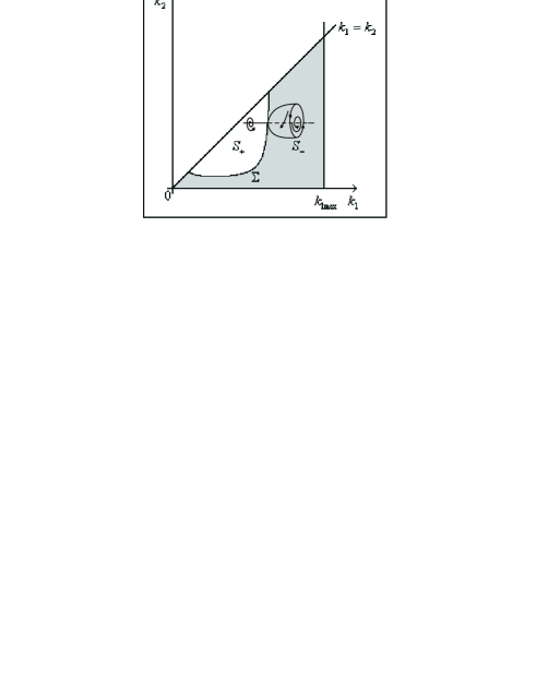
Figure 2: Bifurcation diagram for a typical point on the curve $\Sigma$.

Assuming the same values in the table (28) in next theorem we study the behavior of the Hopf curve $\Sigma$ in the set of admissible parameters $\mathcal{S}$ (see equation (31)) as the parameter $c_{2}$ increases. In fact, the carrying capacity, representing several other factors, has a determinant role on the populations under study.

Theorem 3.3

The one parameter family of curves $\Sigma_{c_{2}}=\Delta_{c_{2}}^{-1}(0)$ has only one point of tangency $T$ with the line $k_{1}=k_{2}$ for $c_{2}=650.41463$. For values $c_{2}>650.41463$ the curve $\Sigma_{c_{2}}$ does not intersect the set $\mathcal{S}$. Therefore for values $c_{2}>650.41463$ the set $\mathcal{S}_{+}$ is empty, $\mathcal{S}=\mathcal{S}_{-}$ and the equilibrium $\mathcal{A}_{4}$ is asymptotically stable for all values $(k_{1},k_{2})\in\mathcal{S}$. See Fig. 3.

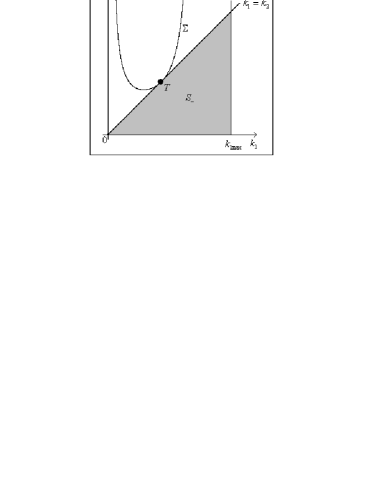
Figure 3: Curve $\Sigma$ intersects $\mathcal{S}$ at one point $T$.

Proof. The surface of Hopf points, or equivalently the one parameter family of Hopf curves, where $J(\mathcal{A}_{4})$ has a pair of purely imaginary eigenvalues is defined by $\Sigma_{c_{2}}=\{\Delta(k_{1},k_{2},c_{2})=0\}$ where $\Delta(k_{1},k_{2},c_{2})$ (see (11)) is given by

$$1699.422-2337.623c_{2}k_{1}-6.860\cdot 10^{7}k_{2}-1114.941c_{2}^{2}k_{1}^{2}-2.175\cdot 10^{12}k_{2}^{2}-$$

$$4.994\cdot 10^{8}c_{2}k_{1}k_{2}-214.747c_{2}^{3}k_{1}^{3}-4.079\cdot 10^{8}c_{2}^{2}k_{1}^{2}k_{2}-1.529\cdot 10^{13}c_{2}k_{1}k_{2}^{2}-$$

$$7.809\cdot 10^{7}c_{2}^{3}k_{1}^{3}k_{2}-4.319\cdot 10^{13}c_{2}^{2}k_{1}^{2}k_{2}^{2}-1.540\cdot 10^{17}c_{2}k_{1}k_{2}^{3}-$$

$$4.755\cdot 10^{6}c_{2}^{4}k_{1}^{4}k_{2}-1.752\cdot 10^{13}c_{2}^{3}k_{1}^{3}k_{2}^{2}-6.741\cdot 10^{17}c_{2}^{2}k_{1}^{2}k_{2}^{3}+$$

$$2.940\cdot 10^{10}c_{2}^{4}k_{1}^{4}k_{2}^{2}-1.703\cdot 10^{18}c_{2}^{3}k_{1}^{3}k_{2}^{3}+1.634\cdot 10^{22}c_{2}^{2}k_{1}^{2}k_{2}^{4}+$$

$$6.618\cdot 10^{16}c_{2}^{4}k_{1}^{4}k_{2}^{3}-4.437\cdot 10^{22}c_{2}^{3}k_{1}^{3}k_{2}^{4}+1.643\cdot 10^{21}c_{2}^{4}k_{1}^{4}k_{2}^{4}.$$

The intersection of the surface $\Sigma_{c_{2}}$ with the plane $k_{1}=k_{2}$ determines the curve $\mathcal{C}$, given implicitly by

$$N(k_{1},c_{2})=1699.422-(2337.623c_{2}+6.860\cdot 10^{7})k_{1}-(1114.941c_{2}^{2}+$$

$$2.175\cdot 10^{12}+4.994\cdot 10^{8}c_{2})k_{1}^{2}-(214.747c_{2}^{3}+4.079\cdot 10^{8}c_{2}^{2}+$$

$$1.529\cdot 10^{13}c_{2})k_{1}^{3}-(7.809\cdot 10^{7}c_{2}^{3}+4.319\cdot 10^{13}c_{2}^{2}+1.540\cdot 10^{17}c_{2})k_{1}^{4}-$$

$$(4.755\cdot 10^{6}c_{2}^{4}+1.752\cdot 10^{13}c_{2}^{3}+6.741\cdot 10^{17}c_{2}^{2})k_{1}^{5}+(2.940\cdot 10^{10}c_{2}^{4}-$$

$$1.703\cdot 10^{18}c_{2}^{3}+1.634\cdot 10^{22}c_{2}^{2})k_{1}^{6}+(6.618\cdot 10^{16}c_{2}^{4}-4.437\cdot 10^{22}c_{2}^{3})k_{1}^{7}+$$

$$1.643\cdot 10^{21}c_{2}^{4}k_{1}^{8}=0.$$

Differentiating implicitly the above expression with respect to $k_{1}$ one has

$$\frac{dc_{2}}{dk_{1}}=-\frac{\frac{\partial N}{\partial k_{1}}}{\frac{\partial N}{\partial c_{2}}}=0,\>\>\frac{d^{2}c_{2}}{dk_{1}^{2}}<0,$$

at $k_{1}=0.00035$ and $c_{2}=650.41463$. Therefore the curve $\mathcal{C}$ is a graph near the point $(k_{1}=0.00035,c_{2}=650.41463)$ and has a local maximum point at $k_{1}=0.00035$. It can be shown [10] that this maximum is global since ${dc_{2}}/{dk_{1}}$ has no other zero. It is easy to verify through a calculation that the point $T=(k_{1},k_{2})=(0.00035,0.00035)$ belongs to $\Sigma_{c_{2}}$ for $c_{2}=650.41463$. Now the gradient of $\Delta_{c_{2}}$ at $T$ for $c_{2}=650.41463$ is given by

$$(-1.73746\cdot 10^{10},1.73746\cdot 10^{10}),$$

which is parallel to the vector $(-1,1)$, the normal to the line $k_{1}=k_{2}$.

$\blacksquare$

Remark 3.4

Since $k_{1_{max}}$ does depend on the parameter $c_{2}$, according to Eq. (7), so does the admissible region $\mathcal{S}=\mathcal{S}_{c_{2}}$. For $c_{2}=650.41463$, a calculation gives $k_{1_{max}}=0.00338491$. This is compatible with position of $T$ at $k_{1}=k_{2}=0.00035$, as illustrated in Figure 3.

4 Concluding Comments

In this paper we studied the system (1) of interest as a mathematical model for biological control, proposed by Yang and Ternes [1, 3, 2] and studied also by Santos [7]. Valuable field data are provided in [3], valid for the citrus leafminer and its native and imported enemies in the region of Limeira (São Paulo, Brazil). An extensive, enlightening discussion of the economic and agricultural interest of the problem, other pertinent differential equations models as well as extensive bibliography, are also presented there.

Under conditions made explicit in Remark 2.1 we determine the unique equilibrium point ($\mathcal{A}_{4}$) with positive coordinates and establish necessary and sufficient conditions for its (Lyapunov) stability (Theorem 2.4). It can be seen however that this condition $\Delta>0$, when expressed in terms of the parameters is a rational function whose denominator does not vanish and its numerator is a polynomial of too many terms to be put in print, but still amenable to numerical calculations. For this reason the treatment of the stability of ($\mathcal{A}_{4}$) in Subsection 3.2 is computer assisted. The conclusion of this study, made precise in Theorem 3.1, is the existence of periodic orbits obtained by Hopf bifurcation, on the side (of $\Delta=0$) where $\mathcal{A}_{4}$ is an attractor.

The study of the general analytic and geometric properties of the boundary of the stability region, given by the Hopf variety $\Delta=0$, so as to include parameter values of biological interest as proposed here as well as others appearing in the work of Ternes [3], remain at the present moment as a mathematical challenge. Theorem 3.3 gives only a thin slice of the geometry.

The reports in [12] and [13], among many others, show that the interest for the combat of the citrus leafminer extends to most regions where citrus trees grow.

The Mathematica notebooks [10], with the table (28), used in the computer assisted arguments for the proofs of Theorems 3.1 and 3.3, can be adapted to tables with data pertinent to other geographic and climatic regions and involving different host–parasitoid interactions.

In [2] Ternes and Yang discuss, with pertinent documentation, the introduction of a foreign parasitoid, Ageniaspis citricola to add the native Galeopsomya Fausta in the combat with the leafminer, Phyllocnistis citrella. They propose a model with eight differential equations for the three species and their immature stages. In [2] and [3] are given starting steps for an analysis of the stability of the equilibria in this extended eight – dimensional system. Based in a numerical study of a complex equilibrium point they recommend that the biological control of the leafminer be implemented with both the native and foreign parasitoids. Meanwhile, the Hopf bifurcation analytic and computer algebra study of the complex equilibria of the eight equations, with the methods used in the present paper, seems unsurmountable at the present moment, due to the large number of parameters involved.

Acknowledgement: The first and second authors developed this work under the projects CNPq Grants 473824/04-3 and 473747/2006-5. The first author is fellow of CNPq. The fourth author is supported by CAPES. This work was finished while the second author visited Universitat Autònoma de Barcelona, supported by CNPq grant 210056/2006-1.

References

-
[1]
H. M. Yang and S. Ternes, Estudo dos efeitos de
dinâmica vital num modelo de controle biológico de pragas
(Study of the effect of the vital dynamics in a model for the
biological control of plagues). Revista de Biomatemática
9, 58-72 (1999) (in Portuguese).
http://www.ime.unicamp.br/7Ebiomat/bio9art_5.pdf -
[2]
H. M. Yang and S. Ternes, Um modelo
determinístico para avaliação do controle biológico de
praga de citros (A deterministic model for the evaluation of the
biological control in plagues of citrus).
Boletim de Pesquisa e Desenvolvimento, Embrapa 3, 1-25 (2002) (in Portuguese).
www.cnptia.embrapa.br/modules/tinycontent3/content/2002/bolpesq3.pdf -
[3]
S. Ternes, Modelagem e simulação da
dinâmica populacional da larva-minadora-da-folha-de-citros em
interação com seus inimigos naturais (Modelling and
simulation of population dynamics of the leafminer in interaction
with its natural enemies), Tese de Doutorado, Faculdade de
Engenharia Elétrica e de Computação, Unicamp, Campinas,
Brazil (2001) (in Portuguese).
http://libdigi.unicamp.br/document/?code=vtls000228128 - [4] H. W. Hethcote, Y. Li and Z. Jing, Hopf bifurcation in models for pertussis epidemiology, Math. Comput. Modelling 30, 29-45 (1999).
- [5] J. A. Jacquez and C. P. Simon, Qualitative theory of compartmental systems, SIAM Review 35, 43-79 (1993).
- [6] H. C. J. Godfray and J. K. Waage, Predictive modelling in biological control: the mango mealy bug (Rastrococcus invadens) and its parasitoids, J. Appl. Ecol. 28, 434-453 (1991).
-
[7]
D. B. Santos, Bifurcação de Hopf num modelo de controle
biológico (Hopf Bifurcation in a biological control model),
Dissertação de Mestrado, Instituto de Matemática e
Estatística, Universidade de São Paulo, São Paulo, Brazil
(2004) (in Portuguese).
http://www.ime.usp.br/~dbraun/dissertacaodanilo.pdf - [8] L. S. Pontryagin, Ordinary Differential Equations, Addison-Wesley Publishing Company Inc., Reading (1962).
- [9] Y. A. Kuznetsov, Elements of Applied Bifurcation Theory, second edition, Springer-Verlag, New York (1998).
- [10] Site with the files used in computer assited arguments in this work: http://www.ici.unifei.edu.br/luisfernando/orange
- [11] S. Wolfram, The Mathematica Book, fifth edition, Wolfram Media Inc., Champaign (2003).
-
[12]
Workshop on the Citrus Leafminer and its Control in the Near
East, F.A.O., Syria, Oct. (1996).
http://www.fao.org/world/Regional/RNE/morelinks/PProt/CLMrpt.pdf
#search=%22Ageniaspis - [13] M. A. Hoy, Proceedings of an International Conference on the Citrus Leafminer, Managing the Citrus Leafminer, Orlando, Florida, April 22-25 (1996).