Experimental Violation of Bell’s Inequality in Spatial-Parity Space

Abstract

We report the first experimental violation of Bell’s inequality in the spatial domain using the Einstein–Podolsky–Rosen state. Two-photon states generated via optical spontaneous parametric downconversion are shown to be entangled in the parity of their one-dimensional transverse spatial profile. Superpositions of Bell states are prepared by manipulation of the optical pump’s transverse spatial parity—a classical parameter. The Bell-operator measurements are made possible by devising simple optical arrangements that perform rotations in the one-dimensional spatial-parity space of each photon of an entangled pair and projective measurements onto a basis of even–odd functions. A Bell-operator value of $2.389\pm 0.016$ is recorded, a violation of the inequality by more than 24 standard deviations.

Introduction—Although Einstein, Podolsky, and Rosen (EPR) Einstein et al. (1935) couched their challenge to the completeness of quantum mechanics in the language of continuous spatial parameters of a two-particle quantum state, most of the subsequent work investigating their claim relied on discrete degrees of freedom Bouwmeester et al. (2000). In particular, Bell Bell (1964) described an approach to delineate quantum theory from those that subscribe to local realism in terms of correlations between two spin-$\frac{1}{2}$ particles. Surprisingly, after more than seventy years of studying the EPR state, the quantum nonlocality potentially exhibited by it has not been experimentally demonstrated in the spatial domain.

While the original paradox has been realized using the EPR state in numerous experiments Ou et al. (1992), including one in the spatial domain Howell et al. (2004), it was posited by Bell himself Bell (1986) that the EPR state should not violate a Bell-type inequality, and hence does not violate local realism, since its associated Wigner distribution Wigner (1932) is positive everywhere. It has since been recognized that this statement is not correct Johansen (1997). The challenge one faces to demonstrate a Bell-inequality violation in the spatial domain is to identify operators that perform rotations and projective measurements on suitably defined observables of the infinite-dimensional Hilbert space associated with the spatial profile of entangled photon pairs. A recent proposal to achieve this Oemrawsingh et al. (2004), relying on orbital angular momentum observables manipulated by spiral phase plates, was subsequently retracted Oemrawsingh et al. (2005). A modified proposal using the same variables Aiello et al. (2005) relies on projecting the EPR state in the spatial domain onto a two-dimensional subspace and has thus far not been demonstrated experimentally; nor have other proposals Larsson (2004). Another approach that retains the entire Hilbert space relies on a set of ‘pseudospin’ operators that have been recently constructed Chen et al. (2002) and that provide a bridge between states described by continuous and discrete variables. In essence, these proposed operators map the infinite-dimensional Hilbert space of the EPR state onto a smaller-dimensional space Brukner et al. (2003). Nevertheless, the physical realization of these operators presents daunting experimental difficulties Chen et al. (2002); Ralph et al. (2000).

In this Letter, we present a conclusive experimental violation of Bell’s inequality in the spatial domain, and thus demonstrate quantum nonlocality using the EPR state produced by spontaneous parametric downconversion (SPDC) Harris et al. (1967). This is made possible by constructing photonic ‘pseudospin’ operators in the spatial domain using an approach that we recently described Abouraddy et al. (2007). These operators make use of the spatial parity (even–odd) of the one-dimensional (1D) transverse field of single photons. This entails mapping the infinite-dimensional Hilbert space of the photon’s transverse spatial profile onto a space of dimension two. It is important to note that the potentially infinite-dimensional Hilbert space of transverse modes (limited by the effective numerical aperture of the experimental arrangement) is mapped onto a two-dimensional space Brukner et al. (2003) and is neither truncated as in Ref. Mair et al. (2001) nor projected onto a smaller-dimensional subspace as in Ref. Aiello et al. (2005).

Spatial-Parity Space—To introduce the above-mentioned mapping, consider a one-photon state in the spatial domain $|\Psi\rangle=\int dx\psi(x)|1_{x}\rangle$, where $\int dx|\psi(x)|^{2}=1$. This state is potentially of infinite dimensionality as governed by the expansion into an orthonormal functional basis $\psi(x)=\sum_{n}c_{n}\xi_{n}(x)$, such that $|\Psi\rangle=\sum_{n}c_{n}|n\rangle$, where $|n\rangle=\int dx\xi_{n}(x)|1_{x}\rangle$. We map this state onto two ‘levels’ of a qubit: the even $\psi_{\textrm{e}}(x)=\frac{1}{2}\{\psi(x)+\psi(-x)\}$ and odd $\psi_{\textrm{o}}(x)=\frac{1}{2}\{\psi(x)-\psi(-x)\}$ components of the photon transverse distribution, which are orthogonal $\int dx\psi_{\textrm{e}}^{*}(x)\psi_{\textrm{o}}(x)=0$. The one-photon state may be recast in the even $|\textrm{e}\rangle$ and odd $|\textrm{o}\rangle$ basis of this 2D space of spatial parity, $|\Psi\rangle=\alpha|\textrm{e}\rangle+\beta|\textrm{o}\rangle$, where $\alpha|\textrm{e}\rangle=\sum_{n}c_{2n}|2n\rangle$ and $\beta|\textrm{o}\rangle=\sum_{n}c_{2n+1}|2n+1\rangle$. The fundamental insight provided in this paper is the isomorphism between the ‘pseudospin’ approach and the that of spatial-parity space.

It has been shown Abouraddy et al. (2007) that the ‘pseudospin’ operators corresponding to the well-known Pauli operators, as well as other relevant operators (such as rotation and projection operators), are easily implementable on this new Hilbert space. The two most relevant operators for this Letter are the parity rotator and the parity analyzer. The parity rotator rotates the state function in parity space, just as a polarization rotator rotates the polarization vector. This operator is implemented using a phase plate that introduces a phase $\theta$ between the $x\geq 0$ and $x<0$ half planes (i.e., having transmissivity $e^{i\frac{\theta}{2}\textrm{sgn}(x)}$), corresponding to a rotation $\theta$ on a Poincaré sphere Abouraddy et al. (2007). The parity analyzer is a device that separates the even and odd components of the state into two separate spatial paths, thus projecting the state onto the even–odd basis. Our implementation of a parity analyzer uses a Mach–Zehnder interferometer (MZI) at zero relative path length delay with a spatial flipper (viz., a device that produces a mirror image of the incident field, $\varphi(x)\rightarrow\varphi(-x)$, implemented in our case by a mirror) inserted in one arm. The resulting interferometer becomes parity sensitive (PS-MZI) Abouraddy et al. (2007); Sasada and Okamoto (2003).

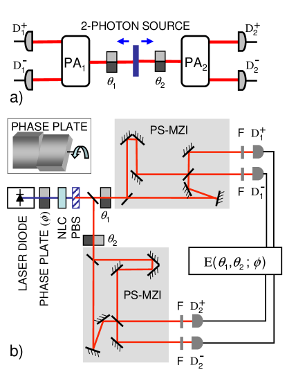
Figure 1: (Color online) (a) Notional configuration for testing Bell’s inequality. PA: parity analyzer; $\theta$: parity rotator; D: detector. (b) Schematic of the experimental arrangement. NLC: nonlinear optical crystal; PBS: polarizing beam splitter; PS-MZI: parity sensitive Mach–Zehnder interferometer; F: interference filter; D avalanche photodetector. The inset depicts the construction of a phase plate (parity rotator) used at three locations in the setup: after the laser diode ($\phi$) and immediately preceding each PS-MZI ($\theta_{1}$ and $\theta_{2}$). It comprises two glass microscope slides, abutted at the origin of the transverse dimension $x=0$ that can be tilted with respect to each other, thus introducing a relative phase between the two halves of the plane.

Experimental Arrangement— A generic configuration for the experimental violation of Bell’s inequality is shown in Fig. 1(a). A two-photon source directs each photon to an SO(2) rotation operator (characterized by angular settings $\theta_{1}$ and $\theta_{2}$) followed by a projective measurement. Coincidence measurements between the detectors $\textrm{D}_{1}$ and $\textrm{D}_{2}$ for various settings of $\theta_{1}$ and $\theta_{2}$ are used to obtain the correlations between a pair of dichotomic outcomes needed for assessing a violation of Bell’s inequality in the CHSH formulation Clauser et al. (1969). In our conception, the SO(2) operator is a parity rotator and the projective measurements on each photon are performed using parity analyzers. Our experimental arrangement is shown schematically in Fig. 1(b). Light from a linearly polarized laser diode (center wavelength 405 nm, power 50 mW) emitting in an even-symmetry spatial mode $\psi_{\textrm{even}}(x)$ is passed through a phase plate that serves as a parity rotator Abouraddy et al. (2007). The angle $\phi$ determines the spatial parity of the exiting pump beam, which illuminates a 1.5-mm-thick $\beta$-barium borate (BBO) nonlinear optical crystal (NLC) in a collinear type-I configuration (signal and idler photons have the same polarization, orthogonal to that of the pump). The collinear signal and idler photons are separated by a beam splitter; each of the exiting photons passes through a parity rotator, set at $\theta_{1}$ and $\theta_{2}$. Each output photon then enters a parity analyzer and then exits to the detectors. The unconverted pump light is removed with the help of a polarizing beam splitter (PBS) placed after the NLC as well as by interference filters F (centered at 810 nm, 10-nm bandwidth) in front of the multimode-fiber-coupled detectors $\textrm{D}_{1}^{+},\,\textrm{D}_{1}^{-},\,\textrm{D}_{2}^{+}\,$ and $\textrm{D}_{2}^{-}$ (EG&G SPCM-AQR-15-FC). It is imprtant to note that we do not couple the photons into single-mode fibers as is the usual practice in projecting orbital angular momentum states onto a single spatial mode Mair et al. (2001); Oemrawsingh et al. (2005); as mentioned above, we aim to collect all the available spatial modes. The outputs of these detectors are fed to coincidence circuits and thence to counters, from which a correlation function E$(\theta_{1},\,\theta_{2};\,\phi)$ (to be defined shortly) is obtained.

Quantum-State Preparation—We produce the different two-photon states investigated here by manipulating the spatial parity of the pump profile $E_{p}(x)$, a classical parameter, via its passage through a phase plate that produces the classical field distribution

$$E_{p}(x)=\cos(\phi/2)\ \psi_{\textrm{even}}(x)+i\,\sin(\phi/2)\ \psi_{\textrm{odd}}(x),$$ (1)

where $\phi$ is the angle of parity rotation imparted by the phase plate to the pump, and $\psi_{\textrm{odd}}(x)=\textrm{sgn}(x)\,\psi_{\textrm{even}}(x)$. The two-photon quantum state produced in 1D by SPDC Harris et al. (1967); Abouraddy et al. (2007) is $|\Psi\rangle=\int\int dxdx^{\prime}\psi(x,x^{\prime})|1_{x},1_{x^{\prime}}\rangle$, where

$$\psi(x,x^{\prime})=E_{p}(\frac{x+x^{\prime}}{2})\xi(\frac{x-x^{\prime}}{2})=\sum_{n=0}^{N}\lambda_{n}\phi_{n}(x)\zeta_{n}(x^{\prime}),$$ (2)

where $\xi(x)$ is a function of width much smaller than that of $E_{p}(x)$, representing the correlation between the emission locations of the two photons, $\sum_{n=0}^{N}\lambda_{n}^{2}=1$, and $\{\phi_{n}(x)\}$ and $\{\zeta_{n}(x)\}$ are two orthonormal sets of functions in the Schmidt decomposition Law and Eberly (2004).

One approach to estimating the number of transverse modes $N$ in the state function’s Schmidt decomposition is to approximate $E_{p}(x)$ and $\xi(x)$ by Gaussian functions with appropriate widths, in which case an analytical expression for $N$ exists Law and Eberly (2004), $N=\frac{1}{4}(w/\sqrt{\lambda_{p}\ell/8}+\sqrt{\lambda_{p}\ell/8}/w)^{2}\approx 4000$, where the pump width $w=1.1$ mm, the NLC thickness $\ell=1.5$ mm, and the pump wavelength $\lambda_{p}=405$ nm. One may also obtain the Schmidt decomposition directly by diagonalizing the function $\eta(x_{1},x_{2})=\int dx^{\prime}\psi^{*}(x_{1},x^{\prime})\psi(x_{2},x^{\prime})$ and counting modes with eigenvalues larger than some threshold, say $\lambda_{n}>0.01\lambda_{\textrm{max}}$, which yields a value of $N\approx 3500$. Thus the state that we use inhabits a Hilbert space of extremely high dimensionality $N\times N$.

The even $\psi_{\textrm{even}}(x)$ and odd $\psi_{\textrm{odd}}(x)$ components of the pump spatial field distribution generate through the process of SPDC the two-photon spatial-parity states $|\Phi^{+}\rangle$ and $|\Psi^{+}\rangle$, respectively, where $|\Phi^{+}\rangle=\frac{1}{\sqrt{2}}\left\{|\textrm{e}\rangle_{1}|\textrm{e}\rangle_{2}+|\textrm{o}\rangle_{1}|\textrm{o}\rangle_{2}\right\}$ and $|\Psi^{+}\rangle=\frac{1}{\sqrt{2}}\left\{|\textrm{e}\rangle_{1}|\textrm{o}\rangle_{2}+|\textrm{o}\rangle_{1}|\textrm{e}\rangle_{2}\right\}$, as detailed in Ref. Abouraddy et al. (2007). This may be understood intuitively by noting that an even-parity (odd-parity) pump results in a Schmidt decomposition of the two-photon state function in Eq. ( 2) composed of a sequence of products of only even–even or odd–odd (even–odd or odd–even) functions. The two-photon state generated by the pump distribution in Eq. (1) is thus

$$|\Psi\rangle=\cos(\phi/2)\,|\Phi^{+}\rangle+i\,\sin(\phi/2)\,|\Psi^{+}\rangle.$$ (3)

It is important to note that this two-photon state is maximally entangled regardless of the value of $\phi$ (the concurrence Hill and Wootters (1997) of the state is unity, independent of $\phi$) and thus allows for a maximal violation of Bell’s inequality.

For the purposes of this Letter only three values of $\phi$ are considered, namely $\phi=0$ (corresponding to an even pump), $\frac{\pi}{2}$ (pump in an equal superposition of even and odd components), and $\pi$ (odd pump), leading to the following two-photon states: $|\Phi^{+}\rangle$, $\frac{1}{\sqrt{2}}\{|\Phi^{+}\rangle+i\,|\Psi^{+}\rangle\}$ and $|\Psi^{+}\rangle$, respectively. A fourth state, $\frac{1}{\sqrt{2}}\{|\Phi^{+}\rangle+|\Psi^{+}\rangle\}$ (i.e., without the factor $i$) is prepared using a pump having the distribution $\frac{1}{\sqrt{2}}\{\psi_{\textrm{even}}(x)+\psi_{\textrm{odd}}(x)\}$. This is achieved by removing the phase plate used to control the pump parity (Fig. 1) and replacing it with an opaque screen that blocks the field on the positive $x$ axis. The resulting two-photon state $\frac{1}{\sqrt{2}}\{|\Phi^{+}\rangle+|\Psi^{+}\rangle\}=\frac{1}{\sqrt{2}}\{|\textrm{e}\rangle_{1}+|\textrm{o}\rangle_{1}\}\otimes\frac{1}{\sqrt{2}}\{|\textrm{e}\rangle_{2}+|\textrm{o}\rangle_{2}\}$ is separable and as such will not violate Bell’s inequality.

Bell-Operator Measurements—After their preparation, each photon in the two-photon states undergoes a rotation in parity space followed by a projective measurement implemented by a phase plate and a PS-MZI, respectively. Photon detection is done in coincidence and the value $+1\ (-1)$ is associated with even (odd) outcomes. One can then estimate the correlation function E$(\theta_{1},\theta_{2};\phi)$ between the parities of the two photons as a function of their respective rotations. It should be noted that the rotation employed here is about an orthogonal axis on the Poincaré sphere to the one often reported in polarization-based experiments. This distinction becomes important when considering tests of quantum physics more stringent than that of Bell Leggett (2003).

Evaluation of the Bell operator in the CHSH form requires measurement of four correlations requiring two settings for each parity rotator

$$\mathcal{B}=\left|\textrm{E}(\theta_{1},\theta_{2})+\textrm{E}(\theta_{1},\theta_{2}^{\prime})+\textrm{E}(\theta_{1}^{\prime},\theta_{2})-\textrm{E}(\theta_{1}^{\prime},\theta_{2}^{\prime})\right|\leqslant 2,$$ (4)

where we omit the implicit dependence on $\phi$ for simplicity. Quantum theory predicts the correlation function for the maximally entangled state given in Eq. (3) to be E$(\theta_{1},\theta_{2};\phi)=\cos(\theta_{1}+\theta_{2}+\phi)$. Accordingly, $\mathcal{B}$ attains the maximum value of $2\sqrt{2}$ when $\theta_{1}=\theta_{2}=\frac{\pi}{8}-\frac{\phi}{2}$ and $\theta_{1}^{\prime}=\theta_{2}^{\prime}=\frac{13\pi}{8}-\frac{\phi}{2}$. When the sate is separable, as is the case for $\frac{1}{\sqrt{2}}\{|\Phi^{+}\rangle+|\Psi^{+}\rangle\}$, the predicted correlation function is E$(\theta_{1},\theta_{2})=0$. The lack of dependence on the setting of either parity rotator can be understood by noting the axis of rotation on a Poincaré sphere. In this case each photon’s state of parity is a point that lies on the axis of rotation chosen in our experimental configuration and the correlation function is thereby unchanged.

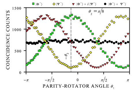
Figure 2: (Color online) Coincidence counts between $\textrm{D}_{1}^{+}$ and $\textrm{D}_{2}^{+}$ as a function of $\theta_{1}$ for fixed $\theta_{2}=\frac{\pi}{8}$ and three values of $\phi$: the green $\blacksquare$ for $\phi=0$ (even pump), the red $\blacktriangledown$ for $\phi=\frac{\pi}{2}$ (pump in equal superposition of even and odd), and the yellow $\blacklozenge$ for $\phi=\pi$ (odd pump). The black $\bullet$ represents the same measurement when the initial phase plate is replaced by an opaque screen that blocks the positive $x$ axis, which leads to a separable two-photon state. A side-effect of the screen is to halve the number of photons produced via SPDC; for purposes of comparison with the previous cases we therefore plotted twice the recorded values in the figure.

Figure 3: (Color online) The correlation function E$(\theta_{1},\theta_{2};\,\phi)$ derived from coincidence measurements for three different maximally entangled two-photon states, corresponding to different settings of the pump parity angle $\phi$ (from left to right $\phi=0$, $\phi=\frac{\pi}{2}$, and $\phi=\pi$). The final (right) panel shows E$(\theta_{1},\theta_{2})$ for a separable state. The dashed white line indicates the cross-section of the data presented in Fig. 2.

Experimental Results—Although evaluation of the Bell operator requires that E$(\theta_{1},\theta_{2};\phi)$ be measured at only four points in the $(\theta_{1},\theta_{2})$ plane; measuring E over the full range of values for $\theta_{1}$ and $\theta_{2}$ provides much more information and offers insight into the effect of the pump parity on the Bell operator. Measurements of the correlation function, for each of the four states prepared, were performed by varying $\theta_{1}$ and $\theta_{2}$ over $2\pi$ radians. Figure 2 provides an example of the coincidence rate recorded by the ‘even’ detectors after the parity analyzers when $\theta_{2}=\frac{\pi}{8}$; the visibility of the recorded coincidence sinusoids for each of the maximally entangled states is $\approx 84\%$. This lower-than-expected visibility is a result of imperfect alignment of the PS-MZIs. The full landscapes for E$(\theta_{1},\theta_{2};\phi)$ are shown in Fig. 3. The functional form of E$(\theta_{1},\theta_{2};\phi)$ for the entangled states are clearly seen to be 2D sinusoids in $\theta_{1}+\theta_{2}$ with the fringes shifted according to the value of $\phi$. The separable state reveals a flat correlation landscape. The measured values of the Bell operator for each state are presented in Table 1. All three entangled states demonstrate clear violations of Bell’s inequality.

Table 1: Measured values of the Bell operator for the four two-photon states investigated, and the amount of the violation of Bell’s inequality.

State	Bell Operator $\mathcal{B}$	Violation
$|\Phi^{+}\rangle$	$2.389\pm 0.016$	$24.2\sigma$
$|\Psi^{+}\rangle$	$2.375\pm 0.018$	$20.5\sigma$
$|\Phi^{+}\rangle+i\,|\Psi^{+}\rangle$	$2.373\pm 0.019$	$19.7\sigma$
$|\Phi^{+}\rangle+\,\,\,|\Psi^{+}\rangle$	$0.057\pm 0.017$	None expected

Conclusion—We have shown that the entangled state proposed in the original embodiment of the EPR paradox violates a Bell inequality in the spatial domain, and thus is at odds with any local-hidden-variables theory. We identified dichotomic observables based on the spatial parity of each particle’s transverse spatial distribution. This identification, combined with our demonstrated abilities to perform rotations in parity space, and projections onto an even–odd basis, enabled us to carry out a direct test of Bell’s inequality in the spatial domain. The results demonstrate clear violations of the bounds imposed by local realism, in agreement with quantum theory.