A New Mechanism for Polarizing Light from Obscured Stars

Abstract

Recent spectropolarimetric observations of Herbig AeBe stellar systems show linear polarization variability with wavelength and epoch near their obscured H_α emission. Surprisingly, this polarization is $not$ coincident with the H_α emission peak but is variable near the absorptive part of the line profile. With a new and novel model we show here that this is evidence of optical pumping – anisotropy of the incident radiation that leads to a linear polarization-dependent optical depth within the intervening hydrogen wind or disk cloud. This effect can yield a larger polarization signal than scattering polarization in these systems.

1 Introduction

Optical polarization measurements may reveal information about the spatially unresolved conditions in the near-environment of stars imbedded in gaseous disks and outflowing winds. Several authors have advanced agendas for using linear polarization measurements to infer the structure of the gas and dust surrounding, for example, Herbig AeBe stars. The analytic models of McLean (1979) used the effects of polarized Thomson scattering and unpolarized line emission to generate variable linear polarization across line profiles. Wood, Brown, and Fox (1993), and Vink et al. (2005) extended this idea in order to predict and model in detail wavelength variations in the polarization near nebular emission lines. Their model accounts for the asymmetry of the nebular scattering and the optical depth dependence of the scattering source. Harries (2000) has also built realistic monte-carlo scattering models of hot-star winds. His results are notable in that they also see absorptive polarization effects that may not be due to the dilution of the scattering polarization from unpolarized line radiation.

Harrington and Kuhn (2007, henceforth HK) observed a sample of 5 Herbig AeBe stars that exhibited significant linear polarization variations in wavelength near the absorptive part of the H_α line. Their largest polarization signal, in AB Aur, was about 1% in the blue absorptive region of the P-Cygni profile, although if expressed as a percentage of the continuum intensity, this is about 0.5%. Even though their measurements were sensitive to linear polarization at the level of a few parts in $10^{4}$, they found negligible polarization variations at the H_α peak emission wavelength. The HK results are problematic for models which depend on line radiation to dilute polarized Thomson scattering, as these models tend to predict significant polarization near the H_α peak emission wavelength. This has led us here to consider resonant scattering models.

Resonant polarized scattering has been considered in the absence of magnetic fields (Warwick annd Hyder 1965) and in the presence of depolarizing magnetic fields through a mechanism known as the Hanle effect (cf. Hanle 1924, Stenflo 1994) and to describe scattering in stellar envelopes (cf. Ignace, Nordsieck, Cassinelli 2004). From a quantum mechanical perspective, resonant scattering polarization is caused by unequal magnetic substate populations within the upper level of an atomic transition. This can be induced by anisotropy of the incident radiation and correlations between the upper sublevels which yields polarization of the scattered/re-radiated light (cf. Stenflo 1998). Resonant scattering alone probably cannot account for the HK observations, but a resonant $absorption$ process appears feasible.

Polarized absorption results if the lower state magnetic atomic sublevels are unequally populated, for example by anisotropic incident radiation. Such an “optically pumped” gas has an opacity that will depend on the electric field direction of the incident flux. Thus, in general, unpolarized light incident on such an absorbing gas can emerge polarized without scattering. Optical pumping has been demonstrated in the laboratory (Happer 1972) and has been discussed in the context of sensitive solar observations (cf. Trujillo Bueno and Landi Degl’Innocenti 1997).

This mechanism has a simple classical explanation when the lower level has, for example, total angular momentum $j=1$ (which is nominally degenerate with magnetic sublevels $m=\pm$1, and 0), and the upper level has $j=0.$ In a cartesian coordinate system we associate the electronic transitions or substates with classical electronic oscillators aligned in the x-y plane (for $\Delta m=\pm$1) and in the $z$ direction (for $\Delta m=0$). We impose a coordinate system with the pumping radiation incident on the gas in the $+z$ direction. Then, only the $\Delta m=\pm 1$ transitions can be excited because the incident transverse electric field lies in the $x-y$ plane. On the other hand the subsequent spontaneous downward transitions equally populate all lower magnetic sublevels. Thus, if there are no collisions to mix sublevels, eventually only the $m=0$ substate will be populated. This case has been analyzed for an anisotropic stellar atmosphere in Trujillo Bueno and Landi Degl’Innocenti (1997).

Now if a second unpolarized beam is incident on the gas in the $+x$ direction (having equal $y$ and $z$ electric field components) only the $z$ component of this electric field is absorbed and scattered by the pumped gas, because only $m=0$ electronic groundstate oscillators are populated. Thus the emergent beam is linearly polarized with a $y$-direction dominant electric field. In general a gas which is anisotropically excited, but is observed with light which is incident from a direction that differs from the optical pumping beam direction, will exhibit an emergent linear polarization with dominant electric field in a direction which is perpendicular to the plane of incidence with the pumping beam. This is the geometry we expect from a star imbedded in a disk or outflowing wind.

When the intervening cloud is optically thin the polarization of the absorbed spectral feature can be larger than any scattered light spectral polarization signal. Figure 1 shows the geometry of a gas cloud near a star of luminosity $L$. Let the cloud and star have radii $r_{c}$ and $r_{s}$ and let the cloud be a distance $d$ from the star. The solid angle subtended by the cloud and the observer’s detector, as seen from the center of the star, are $\Omega_{c}$ and $\Omega_{0}$. The relative polarization of the scattered light signal, $Q_{sc}$, to the total continuum optical signal, $I_{s}$, when the cloud is not projected against the disk of the star, is

$$Q_{sc}/I_{s}={L\Omega_{c}/4\pi~{}f\Omega_{0}/4\pi~{}p_{s}\over L\Omega_{0}/4\pi}~{}=~{}p_{s}f{r_{c}^{2}\over 4d^{2}}$$

where $f$ is the fraction of light incident on the cloud which is scattered (assumed isotropically) and $p_{s}$ is the average intrinsic polarization of this scattered light.

On the other hand, when the cloud lies directly between the disk of the star and the observer, optical pumping can cause the absorbed light to be polarized. Here all the light removed from the beam, by scattering away from the direction to the observer, appears as a polarized absorption spectral feature. This contrasts to the off-disk scattering geometry where it is just the light scattered by the cloud into the small solid angle of the distant detector which is polarized. This absorptive geometry can lead to a larger polarized optical signal. If $r_{c}<r_{s}$ then the relative transmitted polarized flux, $Q_{tr}$, normalized to the total, is

$$Q_{tr}/I_{s}={(r_{c}/r_{s})^{2}L\Omega_{0}/4\pi~{}(1-f)p_{a}\over L\Omega_{0}/4\pi}=p_{a}f{r_{c}^{2}\over r_{s}^{2}}.$$

Here $p_{a}$ is the absorptive (optically pumped) intrinsic polarization which we compute below. The intrinsic scattered polarization $p_{s}$ and $p_{a}$ are due to population differences in, respectively, the upper and lower level magnetic substates, and to the anisotropy of the scattered or pumping radiation. If these intrinsic polarization levels are comparable then the ratio of the total absorptive to scattered polarization is simply ${Q_{tr}/Q_{sc}\approx 4d^{2}(1-f)/fr_{s}^{2}}$. Since the cloud lies above the star, $d$ is always larger than $r_{s}$ and with $f\approx 0.5$ the absorptive polarization signal is (subject to these assumptions) larger than the scattered polarization signal.

Our calculation simplifies the general problem, in particular for the case where the “cloud” has a small line-of-sight velocity with respect to the star. In this case it is not stellar continuum radiation, but H_α emission that optically pumps the intervening gas. In general this enhances the pumping (since H_α can be significantly brighter than continuum) and complicates the geometry (because of the stars rotational doppler shifted photospheric pumping radiation source). Thus our discussion here applies directly to the outflowing wind configuration of, for example, AB Aur. The disk systems HK observed will require a slightly different model.

2 Statistical Equilibrium and H_α

In order to compute the intrinsic absorptive polarization $p_{a}$ we solve the statistical equilibrium equation for the densities of the first 28 (LS coupled) hydrogen energy levels corresponding to all of the principal quantum numbers $n=1,2,3$ and $l=0,1,2$ sublevels. Thus the ground state ($n=1$) consists of an $l=0,~{}j=1/2,~{}m=\pm 1/2$ doublet. The $n=2~{}(l=0,1)$ levels include two $j=1/2$ and one $j=3/2$ states for a total of 8 magnetic substates. Similarly there are 18 $n=3~{}(j=1/2,3/2,~{}5/2)$ sublevels. A 28$\times$28 matrix statistical equilibrium equation is constructed from the radiative transition rates. We note that collisional transitions are unimportant in the density regimes of interest here. The solution for the individual sublevel densities is obtained by a singular value decomposition method.

We first obtain theoretical line strengths and Einstein $A$ and $B$ coefficients for all allowed dipole transitions between individual sublevels (Sobelman 1992). These coefficients describe fixed upper and lower magnetic substates so that stimulated emission and absorption $B$ coefficients for each transition are equal. We check our calculations against the fine structure $A$ coefficents and line strengths listed by NIST (Ralchenko et al. 2007). We again take the quantization axis to lie along the mean incident pumping radiation direction and take the opening half-coneangle as $\theta$. It is the angle-averaged mean radiation intensity that multiplies the Einstein $B$ coefficients in the rate equation. We derive distinct geometrical scaling factors for $\Delta m=0$ and $|\Delta m|=1$ transitions that follow from integrating Stenflo’s (1994) eqns. 3.72 over the pumping radiation solid angle, $\Omega_{s}=\pi\theta^{2}$. For a limb-darkened illuminating stellar disk where $\mu=\cos\gamma$ and $I(\mu)=I_{0}(1-a+a\mu)$ we obtain factors $C_{|\Delta m|}(\theta)$ that multiply the pumping blackbody background radiation terms in the rate equation. We find $C_{0}(\theta)=(1-a)(1/2-3\cos{\theta}/4+\cos^{3}{\theta}/4)~{}+~{}a(3/8(1-\cos^{2}{\theta})+3\cos^{4}{\theta}/16)$ and $C_{1}(\theta)=(1-a)(1/2-3\cos{\theta}/8-\cos^{3}{\theta}/8)~{}+~{}a(9/16-3\cos^{2}{\theta}/16-3\cos^{4}{\theta}/32)$. We use the theoretical limb-darkening coefficients from Al-Naimiy (1978).

Anisotropy of the illuminating stellar light source leads to a difference in the $m=\pm 3/2$ and $m=\pm 1/2$ populations (within the $n=2,~{}j=3/2$ level). This lower state anisotropy linearly polarizes the transmitted light from the star which passes through the cloud at a non-zero angle, $\gamma$, with respect to the $z$ (optical pumping) direction. Given the geometry defined by Fig. 1 we expect the emergent light to be partially polarized with electric field perpendicular to the plane of the figure. Most astronomical observations do not resolve the fine structure of the $n=2$ to $n=3$ H_α line but they will still exhibit a diluted linear polarization signal because only some of the transitions are insensitive to the pumping radiation anisotropy (e.g. those which start and end on $j=1/2$ levels).

3 Polarized Radiative Transfer in the Intervening Cloud and the Form of the Polarization Solutions

The Stokes transfer equation simplifies in our geometry where the stellar photosphere is a background light source and the intervening cloud is optically thin. We take the positive Stokes $Q$ direction to correspond to light with electric field perpendicular to the plane of Figure 1. The Stokes vector transfer equation (cf. eq. 11.1 Stenflo 1994) involves only $I$ and $Q$ intensity, and $\eta_{I}$ and $\eta_{Q}$ continuum-normalized opacity terms. Since the stellar photospheric background is the only source of photons observed through the cloud, there are no source or emissivity terms to consider in the polarized transfer equation.

Harrington and Kuhn (2007) detected only small polarization ($Q<<I$) in the stellar systems they observed. In this approximation, the transfer equation reveals that light transmitted through a diameter of the cloud will have polarization $p_{a}=Q/I=\Delta Q/I~{}\approx 2r_{c}\eta_{Q}\kappa_{cont}$ where $\kappa_{cont}$ is the normalizing continuum opacity. Here $I$ is the continuum intensity and we compute $\eta_{I,Q}\propto n_{I,Q}$ from the lower level population anisotropies and eqns. 3.74 (Stenflo 1994). In this case the effective refractive index and opacity terms $n_{0,\pm}$ or H_0,± (eqn 4.41) are computed from sums of the products of the $B$ coefficients and the sublevel populations, derived separately for the $\Delta m=\pm 1$ and $\Delta m=0$ transitions. The optical depth through the cloud is just $\tau=2r_{c}\eta_{I}\kappa_{cont}\approx-\log{(1-f)}$ where $f$ is the fraction of H_α photons scattered, as defined above. We find that for clouds with typical path lengths of, say, $r_{s}$ the optically thin condition yields hydrogen densities that are effectively collisionless.

In the low density conditions of this disk/wind the statistical equilibrium rate equation depends on only stimulated emission, absorption, and spontaneous emission processes. It is the difference in the angular dependence of the $\Delta m=0$ versus $|\Delta m|=1$ coupling to the anisotropic radiation field that leads to differences in the degenerate $n=2$ magnetic sublevel populations. Several qualitative features of the optical pumping solutions are intuitive. For intense pumping radiation fields the anisotropy yields a decreasing absorptive polarization – in this regime the spontaneous emission is negligible and the net upward and downward transition rates between any two levels must be the same. In this case the equilibrium level populations are independent of the upward/downward transition rates. Consequently there can be no sublevel density differences and the absorptive polarization must vanish. Similarly for weak radiation fields it is the spontaneous emission that defines transition rates and this term in the rate equation does not depend on the radiation anisotropy. Thus at low and high radiation backgrounds the absorptive polarization approaches zero.

The absorptive polarization near H_α is also a function of the ratio of the H_α to $L_{\beta}$ (and $L_{\alpha}$) pumping flux. The ratio of the $n=2,~{}j=3/2$ to $j=1/2$ populations affects the net H_α polarization, since only the $j=3/2$ states are sensitive to radiation anisotropy. In the limit of no background H_α flux (and in the absence of collisions) all the hydrogen ends up in the “sterile” $n=2~{}l=0$ state because it has no decay route and there is no radiative absorption to depopulate it. Conversely, as the pumping H_α flux increases the equilibrium $n=2~{}j=3/2$ levels are populated and the induced linear polarization can increase.

This results in a rather weak temperature dependence of the optical pumping source on the absorptive polarization. Even though a decreasing source temperature decreases the pumping radiation, this effect on the polarization is compensated by the increasing ratio of H_α to $L_{\beta}$ flux. We find that between 30,000 to 3,000K, a change in pumping flux by nearly 4 orders of magnitude, the absorptive polarization is nearly constant. For example, a cloud located 1.1 stellar radii from a 30,000K star ($\theta=65\arcdeg$) that is $\gamma=65\arcdeg$ from the line-of-sight to the center of the star, yields linear polarization of 0.53%. If the star has a temperature of 3000K the polarization only decreases to 0.48%.

For fixed radiation mean intensity, as the pumping half-cone angle ($\theta$) increases the anisotropy decreases and the polarization decreases. This effect continues until $\theta=90\arcdeg$, at which point there is no difference between the dipole coupling of radiation to $\Delta m=0$ and $|\Delta m|=1$ transitions. The actual level population difference scales with $\theta$ as the difference between the derived geometric radiation coupling coefficients $C_{0}(\theta)$ and $C_{1}(\theta)$ defined above. It is straightforward to see that this varies like $\theta^{2}$ at small angles. Thus the linear polarization $decreases$ for small cone angles (even though the anisotropy increases). This is because the pumping radiation intensity declines rapidly with $\sin{\theta}=1/d$ (where $d$ is in units of the stellar radius) as the cloud-star distance increases. Figure 2 shows how the linear polarization varies for a cloud seen at the projected edge of a star, as a function of the cloud-star distance, $d$. At small distances from the star the limb darkening function yields significant anisotropy that keeps the polarization from going to zero.

The absorptive polarization depends strongly on the angle between the absorbed beam and the mean pumping direction. As this angle ($\gamma$) increases the polarization perpendicular to the plane increases. For example, with a $T=10,000K$ source temperature and a $65\arcdeg$ cone angle the polarization increases almost linearly from $0$ to $0.5\%$ as $\gamma$ varies from $0$ to $65\arcdeg$.

4 Specific Solutions

We are developing detailed forward solutions for all the HAeBe stars we have observed and to account for stellar emission line pumping. Here it is interesting to describe the general form of the wavelength dependent linear polarization expected from an intervening wind or disk structure. We consider two geometries; a radial outflow and a rotating disk illuminated (optically pumped) by the stellar blackbody. The geometry is essentially that defined in Fig. 1 but we allow that the wind or disk’s symmetry axis is inclined at an angle $b$ with respect to the line-of-sight to the star. We rotate the common plane containing the line-of-sight direction and the symmetry axis to be oriented vertically. Then, as seen from the observer, the intervening cloud projects onto a horizontally oriented arc across the stellar disk. The disk is both illuminated by the star and absorbs the stellar light behind it. Each point on this arc contributes absorptive polarization at a distinct velocity with respect to the observer.

We take positive Stokes $Q$ along the vertical sky direction. Positive $U$ corresponds to an electric field that is $45\arcdeg$ to this. It follows that the absorptive polarization of a symmetric radial wind should yield only $+Q$ polarization at all velocities. In Figure 3 we’ve plotted the $Q$ polarization across the velocity distribution of the intervening outflow in units of the maximum (assumed spatially constant) outflow velocity. This is illustrative, although most real stellar disks and outflows are not expected to be homogeneous in density or velocity. In general we expect (and observe) a non-zero $U$ polarization which, of course, depends on the rotation angle between the instrument $Q$-axis and the star. The zero polarization level is also ill-defined in the observations since a wavelength independent constant has been removed. Nevertheless the polarization amplitude and simple form of AB Aur in the HK data is consistent with the “diamond” symbols in Fig. 3.

In contrast, even a homogeneous rotating disk geometry must exhibit non-zero $Q$ and $U$ line profiles because the zero line-of-sight velocity condition occurs along the vertical symmetry line near the peak of the H_α emission. The characteristic symmetric (about zero relative velocity) Stokes $Q$, and antisymmetric $U$ profiles for such a disk are also plotted in Figure 3. These are plotted against units of the maximum rotation or outflow velocity of the disk or wind. The polarization outside of these plotted points must be zero, but spectral smoothing due to the finite spectral resolution of the measurements will yield some polarization outside of the absorptive region.

5 Conclusions

This new model shows how optical pumping can describe the magnitude and form of the absorptive linear polarization features recently seen in some obscured stellar systems. The variation of $Q$ and $U$ linear polarization detected near H_α originates from the intervening gas cloud projected against the disk of the star. The polarization features contain information on the kinematics and inclination of the cloud. One immediate conclusion from these calculations is that the absorptive region is near the surface of the star, most likely within 2 stellar radii in order to have a polarization amplitude of about 0.5% . For constrained geometries it may be possible to devise an inversion technique to extract more specific information on non-homogeneous cloud structures in the innermost regions of these stellar systems.

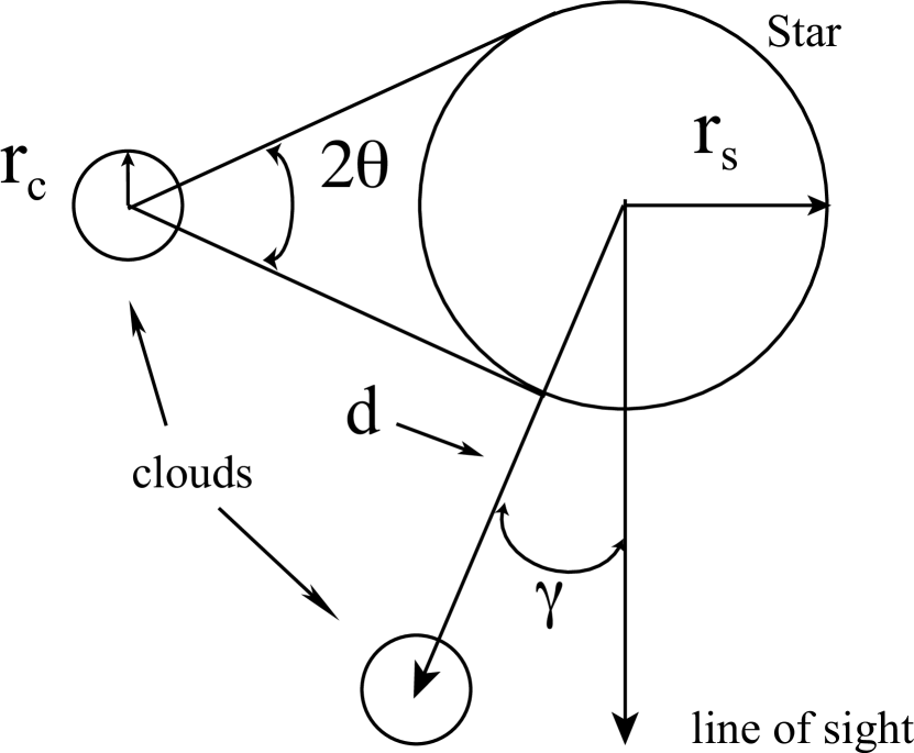
Figure 1: Off-limb and intervening gas cloud geometries that yield H_α polarization

Figure 2: Polarization as a function of distance, $d$, between cloud and star assuming a T=10,000K A star, limb darkening, and with the intervening cloud at the projected edge of the stellar disk at the indicated radial distance from the star center.

Figure 3: Stokes $Q/I$ (plus symbols) and $U/I$ (star symbols) polarization versus relative velocity of a rotating hydrogen disk. The disk inclination angle is $b=80^{o}$, $T=10000$K, and $d=1.1r_{s}$. The $Q/I$ polarization for a comparable outflowing wind is plotted with “diamond” symbols against units of the relative maximum outflow velocity. The peak H_α emission occurs at zero in the horizontal axis units and the polarization signal in each case is zero outside of the plotted points for that geometry.

References

- a (78) Al-Naimiy, H. M. 1998, Ap& SS, 53, 181A
- h (24) Hanle, W. 1924, Z. Phys., 30, 93
- h (72) Happer, W. 1972, Rev. Mod. Phys. 44, 169
- h (07) Harrington, D.M., Kuhn, J.R. (ApJ Letts. in review)
- b (00) Harries, T. J. 2000, Mon. Not. R. Astron. Soc., 315, 722.
- i (04) Ignace, R., Nordsieck, K., Cassinelli, J.P. 2004, Ap. J., 609, 1018
- m (79) McLean, I.S. 1979, Mon. Not. R. Astron. Soc., 186, 265
- r (07) Ralchenko, Y. et al. 2007, NIST Atomic Spectra Database version 3.1.2 [available online at http://physics.nist.gov/asd3]
- s (92) Sobelman, I.I. 1992, Atomic Spectra and Radiative Transitions (Berlin: Springer)
- s (94) Stenflo, J.O. 1994, Solar Magnetic Fields (Dordrecht: Kluwer)
- s (98) Stenflo, J.O. 1998, A& A, 338, 301
- t (97) Trujillo Bueno, J., Landi Degl’Innocenti, E. 1997 ApJ 482, L183
- vi (05) Vink, J. S., Harries, T.J., Drew, J. 2005, A& A, 430, 213
- w (65) Warwick, J.W., Hyder, C. 1965, Ap. J., 141, 1362
- wbf (93) Wood, K., Brown, J.C., Fox, G. 1993, A& A, 271, 492