Spin Injection in Quantum Wells with Spatially Dependent Rashba Interaction

Abstract

We consider Rashba spin-orbit effects on spin transport driven by an electric field in semiconductor quantum wells. We derive spin diffusion equations that are valid when the mean free path and the Rashba spin-orbit interaction vary on length scales larger than the mean free path in the weak spin-orbit coupling limit. From these general diffusion equations, we derive boundary conditions between regions of different spin-orbit couplings. We show that spin injection is feasible when the electric field is perpendicular to the boundary between two regions. When the electric field is parallel to the boundary, spin injection only occurs when the mean free path changes within the boundary, in agreement with the recent work by Tserkovnyak et al. [cond-mat/0610190].

I Introduction

Spintronics envisions electronic devices with spin injection, detection, and manipulation. The spin-orbit interaction couples the electron spin to its orbital motion. It was early realized that it can be utilized to manipulate the electron spin in e.g. the Datta-Das spin transistor.Datta:apl90 More recently, the possibility of spin injection via the spin-orbit interaction in non-magnetic systems was suggested.Hirsch:prl99 ; Murakimi:science03 The spin-orbit interaction gives rise to the spin Hall effect where a longitudinal electric field induces a transverse spin current. In semiconductors, the spin Hall effect has generated a large interest and is predicted to occur in a wide variety of electron and hole doped 2D and 3D systems. Sinova:prl04 A resulting accumulation of a normal to 2DEG spin polarization near sample boundaries has recently been measured.Kato:science04 Also, injection of the spin Hall polarization into a region of the 2DEG where the driving electric field is absent has been observed in Ref. SihAwschalom _injection, .

The spin Hall effect is conventionally separated into an intrinsic and an extrinsic effect. The intrinsic spin Hall effect is caused by the spin-orbit splitting of energy bands in zinc-blende semiconductors. In contrast, the extrinsic spin Hall effect arises due to spin-dependent scattering off impurities. This paper considers the intrinsic spin Hall effect in the diffusive transport regime for electrons confined in a quantum well subject to the Rashba spin-orbit interaction. We will focus on spin diffusion in systems where the Rashba coupling constant $\alpha$ varies in space. In particular, we address a problem of injection of the spin polarization from regions with a large spin-orbit coupling $\alpha$ to regions where this constant is small or zero.

Recent research has established how spins diffuse, precess and couple to the charge transport in electron doped III-V semiconductor quantum wells. The charge and spin flows are described by spin-charge coupled diffusion equations. Burkov:prb04 ; Mischenko:prl04 However, the diffusion equations, valid in the bulk of the systems, must be supplemented by appropriate boundary conditions. Calculations to this end were carried out in Refs. Adagideli:prl05, ; Malshukov:prl05, ; Galitski:prb06, ; Bleibaum:prb06.1, ; Bleibaum:prb06.2, ; Rashba:physica06, and have given rise to discussion in recent literature. The derivation of these boundary conditions is more subtle than it might first seem since the calculations must be carried out to the second order in the spin-orbit interaction strength and include the effects of the electric field.

The correct boundary condition when the electric field is parallel to the boundary and the spin-orbit coupling varies in space was derived in Ref. Tserkovnyak, . An argument in terms of conventional Hall physics that extends the results to systems where also the mobility varies was also given: A spatially dependent spin-orbit coupling varying on length scales smaller than the spin-precession length corresponds to an effective magnetic field of opposite magnitude for two spin directions.Tserkovnyak ; Tserkovnyak:cm0611086 The effective magnetic field induces spin dependent Hall voltage across the boundary.Tserkovnyak This additional voltage, in its turn, gives rise to the spin density variation in the transition layer, resulting in a finite spin-density jump, when the transition layer thickness is reduced to zero.

This paper aims to address spin diffusion and the boundary conditions in more detail and generality for the Rashba spin-orbit interaction model. Our aim is to clarify some conceptual issues and not to fit experimental data because typical experimental systems are rather complex with competing effects and material parameters that are not well known. The Rashba spin-orbit interaction in semiconductor quantum wells depends on quantum well confinement, which can be manipulated by gates, or doping profile, Nitta97 but usually only at rather long scales. The length scales for variations in system properties such as the spin-orbit interaction and the mean free path are typically much larger than the mean free path. Therefore, we will derive general diffusion equations that are valid when the system parameters vary on length scales longer than the mean free path. These diffusion equations can then be solved for smooth boundaries between regions of different spin-orbit coupling strengths and mean free path. From these solutions, we will find boundary conditions that are not limited to a specific relative direction between the electric field and the interface. When the electric field is parallel to the interface our derived boundary conditions agree with the result by Tserkovnyak et al.Tserkovnyak and the analog with conventional Hall physics is rigorously justified beyond the simplest scenario considered microscopically in Ref. Tserkovnyak, . We also present results for the boundary conditions when the electric field is perpendicular to the interface.

Our paper is organized in the following way. In the next section II, we summarize our main results for the resulting boundary conditions between regions with different spin-orbit couplings and mean free path. We discuss the implications of these boundary conditions on spin injection and show that for a parallel electric field spin injection is only possible when the mean free path together with $\alpha$ vary within the boundary layer, while for the perpendicular field spin injection takes place even when the mean free path is uniform in the system. Using the Keldysh formalism, we derive the general diffusion equation in section III that we employ to compute the boundary conditions presented in section II. Our conclusions are in section IV.

II Boundary conditions and spin injection

In the absence of disorder, the electrons in a homogeneous quantum well are described by the Hamiltonian

$$H=\frac{\hbar^{2}\mathbf{k}^{2}}{2m^{\ast}}+\bm{\sigma}\cdot\mathbf{h}_{\mathbf{k}},$$ (1)

where $m^{\ast}$ is the electron effective mass, $\mathbf{k}=\left(k_{x},k_{y}\right)$ is the wave vector, $\bm{\sigma}$ is a vector of Pauli matrices, and $\mathbf{h}_{\mathbf{k}}$ is the effective spin-orbit field. Let us assume that the major contribution to the spin-orbit interaction (SOI) is given by the Rashba interaction:

$$h_{\mathbf{k}}^{x}=\alpha k_{y}\,\,\,,\,\,\,h_{\mathbf{k}}^{y}=-\alpha k_{x}\,,$$ (2)

where $k_{i}$ is the 2D electron wave vector. We also assume that the spin-orbit coupling constant $\alpha(\mathbf{r})$ is spatially modulated. In this case, the spin orbit term in Eq. (1) has to be modified to preserve the Hermitian form of the Hamiltonian, namely, this term is rewritten as 1/2 of the anticommutator of the momentum operator and the spatially dependent $\alpha(\mathbf{r})$.

Since the spatial variations of $\alpha$ are assumed to be provided by an appropriate quantum well modulation or impurity doping profile, any consistent model must in general also take into account spatial variations of the mean free scattering time $\tau(\mathbf{r})$. The electron gas is under the action of the electric field $\mathbf{E}(\mathbf{r})$ and our goal is to find the spin density induced in the 2DEG by $\mathbf{E}$. The electric field may vary in regions where the mobility changes in order to maintain a constant charge current density. We will derive the general diffusion equations corresponding to the Hamiltonian (1) in the next section (III).

Let us first discuss some of our main findings of the general diffusion equations when applied to the problem of spin injection from a region with a large spin-orbit coupling to a region with a smaller spin-orbit coupling. As an example, we consider a left ($x<-d/2$) and right region ($x>d/2$) with different spin-orbit couplings and mean free paths connected via a smooth transition layer, as shown in Figure 1.

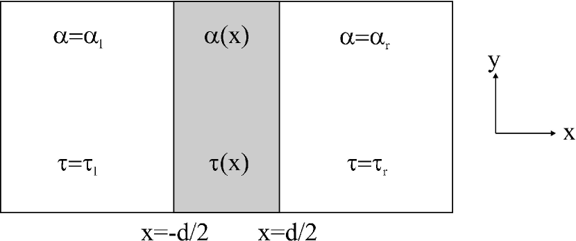
Figure 1: A 2DEG with a spatial dependent Rashba interaction and scattering time. The Rashba interaction $\alpha(x)$ and scattering time $\tau(x)$ vary in the transition region between the left region where $\alpha=\alpha_{l}$ and $\tau=\tau_{l}$ and the right region where $\alpha=\alpha_{r}$ and $\tau=\tau_{r}$.

We assume that the transition layer thickness $d$ between the regions is larger than the mean free path $l$, but smaller than the spin precession length $\lambda=\hbar^{2}/m^{*}\alpha$, where $m^{*}$ is the electron effective mass, $l\ll d\ll\lambda$. This requires a sufficiently weak spin-orbit interaction or a low mobility sample. We consider the general case where the electric field is in the two dimensional plane, $\mathbf{E}=E^{x}\mathbf{x}+E^{y}\mathbf{y}$.

The diffusion equations for the spin-components $S^{x}$, $S^{y}$, and $S^{z}$ of the spin accumulation in the bulk of each region ($x<-d/2$ or $x>d/2$) valid when $1/\tau,h_{k_{F}}\ll E_{F}$ are Burkov:prb04 ; Mischenko:prl04 ; Malshukov:prl05

$$D\nabla^{2}S^{x}+4Dm^{\ast}\alpha\nabla S^{z} = \Gamma_{\parallel}\left(S^{x}-S_{b}^{x}\right)\,,$$

$$D\nabla^{2}S^{y} = \Gamma_{\parallel}(S^{y}-S_{b}^{y})\,,$$

$$D\nabla^{2}S^{z}-4Dm^{\ast}\alpha\nabla S^{x} = \Gamma_{\perp}S^{z}\,,$$ (3)

where $D=v_{F}^{2}\tau/2$ is the diffusion constant in terms of the Fermi velocity $v_{F}$ and the elastic scattering time $\tau$ and $\Gamma_{\perp}=2\Gamma_{\parallel}=8D\left(m^{\ast}\right)^{2}\alpha^{2}$ are the D’yakonov-Perel spin relaxation rates. It is well known that in systems with Rashba interaction, a uniform electric field induces a nonequilibrium bulk spin polarization parallel to the 2DEG,Edelstein denoted in Eqs. (3) as $S_{b}^{x}$ and $S_{b}^{y}$. Within the linear response theory, the spin polarization components are

$$S_{b}^{x} = -\alpha eE^{y}\tau N_{F},$$

$$S_{b}^{y} = \alpha eE^{x}\tau N_{F},$$

where $N_{F}=m^{\ast}/(\hbar^{2}2\pi)$ is the density of states at the Fermi energy. The spin current is not a conserved quantity in spin-orbit coupled systems, but, with the conventional definition within the semiclassical theory,Tang:prb05 it reads in diffusive systems for spin flow, e.g., along the $x$ direction:Malshukov:prl05

$$j^{x} = D\left[\nabla_{x}S^{x}+2m^{\ast}\alpha S^{z}\right],$$

$$j^{y} = D\nabla_{x}S^{y},$$

$$j^{z} = D\left[\nabla_{x}S^{z}-2m^{\ast}\alpha\left(S^{x}-S_{b}^{x}\right)\right]\,.$$

We generalize below the diffusion equations (3) to systems with spatially varying parameters $\alpha$ and $\tau$.

By solving these generalized diffusion equations in the boundary transition layer ($-d/2<x<d/2$), that is thinner than the spin-precession length $\lambda$, we find in Sec. III the boundary conditions

$$\left(S^{x}-S_{b}^{x}\right)_{d/2}-\left(S^{x}-S_{b}^{x}\right)_{-d/2} = -\!\int_{-d/2}^{d/2}\!\!\!\!\!\!\!\!dxS_{b}^{x}\frac{1}{\tau}\frac{d\tau}{dx}\,,$$ (4)

$$S^{y}_{d/2}-S^{y}_{-d/2} = 0,,$$ (5)

$$S_{d/2}^{z}-S_{-d/2}^{z} = 0\,.$$ (6)

The boundary condition for the $S^{x}$ spin density component can be understood in terms of a conventional Hall effect for two spin directions in the transition layer, see the discussion in Ref. Tserkovnyak, . We outline in the next section III how the boundary condition for the $S^{y}$ component can be understood as a result of electron drift in an effective spin dependent potential.

The boundary condition for the spatial derivative of the spin density is particularly simple. It can be written as continuity of spin current in its conventional definition:

$$\left(\mathbf{j}_{s}\right)_{d/2}-\left(\mathbf{j}_{s}\right)_{-d/2}=0$$ (7)

Naively, the continuity of the spin current across the boundary is not surprising because the boundary conditions have been obtained assuming that the boundary layer is thinner than the spin precession length. That means that effects violating spin current conservation only occur on much larger length scales. Consequently, there is spin current conservation through the boundary. However, the continuity of the spin current across the boundary cannot be rigorously established without doing an actual calculation. There could in general be a violation of the spin current conservation of the order $\alpha^{2}$, but we find explicitly in the next section III that also such corrections are absent.

Let us now discuss the implications of the diffusion equations (3) and the boundary conditions (4), (5), (6), and (7) for spin injection from a region with e.g. a larger spin-orbit coupling constant to a region with a smaller spin-orbit coupling constant. We consider two limits for the alignment between the electric field and the boundary: 1) The electric field is parallel to the boundary, $\mathbf{E}=E^{y}\mathbf{y}$, $E^{x}=0$ and 2) the electric field is perpendicular to the boundary, $\mathbf{E}=E^{x}\mathbf{x}$, $E^{y}=0$. Since we consider the linear response regime, spin injection for general orientations between the electric field and the boundary can be found as a linear combination of 1) and 2).

The former case 1) of a parallel electric field $\mathbf{E}=E^{y}\mathbf{y}$ corresponds to the case studied by Tserkovnyak et al.Tserkovnyak For this geometry, the bulk nonequilibrium spin accumulation along the $y$ direction vanishes, $S_{b}^{y}=0$, and the boundary condition (5) implies that

$$S^{y}=0$$

throughout the system. The only nonvanishing bulk component of the spin distribution is along $x$. Deep inside the bulk of the left (l) and right (r) regions:

$$S_{b_{l}}^{x} = -\alpha_{l}eE^{y}\tau_{l}N_{F},$$

$$S_{b_{r}}^{x} = -\alpha_{r}eE^{y}\tau_{r}N_{F}.$$

If the electron mobility is the same in each region, $\tau_{l}=\tau_{r}$, and constant throughout the boundary, then the spin accumulation $S^{x}$ will change rapidly (i.e., on the scale of the spatial variations of $\alpha$, $d$) from $S_{b_{l}}^{x}=-\alpha_{l}eE^{y}\tau_{l}N_{F}$ at $x=-d/2$ to $S_{b_{r}}^{x}=-\alpha_{r}eE^{y}\tau_{r}N_{F}$ at $x=d/2$. For the slowly varying $S^{x}$ in bulk, this looks as a discontinuity in the spin accumulation at the boundary. When the mobility differs in the two regions, the magnitude of discontinuity in the spin accumulation across the boundary is modified according to Eq. (4). This result differs from Ref. Adagideli:prl05, , where a continuous spin density across the boundary was assumed. Solving the diffusion equations (3), the solution in the left region is ($x<-d/2$) Burkov:prb04

$$S^{x} = S_{b_{l}}^{x}+\sum_{n=1,2}S_{i_{l},n}^{x}\exp q_{l,n}\left(x+d/2\right)\,,$$

$$S^{z} = \sum_{n=1,2}S_{i_{r},n}^{z}\exp q_{l,n}\left(x+d/2\right)$$

and in the right region ($x>d/2$)

$$S^{x} = S_{b_{r}}^{x}+\sum_{n=1,2}S_{i_{r},n}^{x}\exp q_{r,n}\left(-x+d/2\right)\,,$$

$$S^{z} = \sum_{n=1,2}S_{i_{r},n}^{z}\exp q_{r,n}\left(-x+d/2\right),$$

where $q_{n}$ is the solution with positive real part of $q_{n}=(1/\lambda)\sqrt{2(-1\pm i\sqrt{7})}$. Continuity of the spin current, Eq. (7), combined with the boundary conditions for $S^{x}$ and $S^{z}$, Eqs. (4) and (6), imply

$$S_{i_{l},n}^{x} = \varkappa_{l,n}^{x}\Delta S^{x}\,,$$

$$S_{i_{r},n}^{x} = \varkappa_{r,n}^{x}\Delta S^{x}\,,$$

$$S_{i_{l},n}^{z} = \varkappa_{l,n}^{z}\Delta S^{x}\,,$$

$$S_{i_{r},n}^{z} = \varkappa_{r,n}^{z}\Delta S^{x}\,,$$

where

$$\Delta S^{x}=-\!\int_{-d/2}^{d/2}\!\!\!\!\!\!\!\!dxS_{b}^{x}(x)\frac{1}{\tau}\frac{d\tau}{dx}$$

and $\varkappa_{l}^{x}$, $\varkappa_{r}^{x}$, $\varkappa^{z}_{l}$ and $\varkappa^{z}_{r}$ are lengthy algebraic dimensionless coefficients that depend on $q_{l,n}$, $q_{r,n}$ and the diffusion coefficients $D_{l}$ and $D_{r}$. From these boundary conditions, it should be clear that spin injection, which we define as a spin accumulation that differs from the bulk spin density ${\bf S}_{b}$, i.e., $S_{i}\neq 0$, is only feasible when the mobility varies within the boundary layer, since otherwise $\Delta S^{x}$ vanishes. If the mobility is constant throughout the system, there is no spin injection from the left region to the right region or vice versa. In general, $\Delta S^{x}$ depends on the specifics of the variation of the mobility and the spin-orbit coupling in the boundary layer.

Next, let us study the second scenario 2) where the electric field is perpendicular to the boundary, $\mathbf{E}=E^{x}\mathbf{x}$, $E^{y}=0$. In this case, we will find that spin injection is feasible even when the mobility is uniform throughout the system. In the bulk of the left (right) region, we have $S^{y}=S_{b_{l}}^{y}=\alpha_{l}eE^{x}_{l}\tau_{l}N_{F}$ ($S^{y}=\alpha_{r}eE^{x}_{r}\tau_{r}N_{F}$), while the other spin components vanish. Since the electric current is continous across the interface, the electric fields on both sides of the boundary must differ in order to adjust to the different mobilities so that $E^{x}_{l}\tau_{l}=E^{x}_{r}\tau_{r}$. The boundary conditions (4), (6), and (7) then imply that

$$S^{x}=0\,\,\,{\rm and}\,\,\,S^{z}=0$$

throughout the system. In contrast to the previous scenario 1), where the in-plane spin component $S^{x}$ exhibits a discontinuity across the transition layer when the mobility is uniform, $S^{y}$ is continous here. Solving the diffusion equations (3), we find in the left region ($x<-d/2$)

$$S^{y}=S_{b_{l}}^{y}+S_{i_{l}}^{y}\exp\lambda_{l}^{-1}\left(x+d/2\right),$$

and in the right region ($x>d/2$)

$$S^{y}=S_{b_{r}}^{y}+S_{i_{r}}^{y}\exp\lambda_{r}^{-1}\left(-x+d/2\right),$$

Continuity of the spin current and the boundary condtions for $S^{y}$ imply

$$S_{i_{l}}^{y} = \varkappa_{l}^{y}\left[-\left(S_{b_{r}}^{y}-S_{b_{l}}^{y}\right)\right]$$

$$S_{i_{r}}^{y} = \varkappa_{r}^{y}\left[-\left(S_{b_{r}}^{y}-S_{b_{l}}^{y}\right)\right]$$

where

$$\varkappa_{l}^{y} = -\frac{D_{r}\lambda_{r}^{-1}}{D_{l}\lambda_{l}^{-1}+D_{r}\lambda_{r}^{-1}},$$

$$\varkappa_{r}^{y} = \frac{D_{l}\lambda_{l}^{-1}}{D_{l}\lambda_{l}^{-1}+D_{r}\lambda_{r}^{-1}}\,.$$

In the limit of weak spin-flip relaxation in the left region, $\lambda_{l}\gg\lambda_{r}D_{l}/D_{r}$, we find $\varkappa_{l}^{y}=-1$, $\varkappa_{r}^{y}=0$ and $\varkappa^{z}=0$. In contrast to scenario 1), spin injection is feasible even when the mobility is constant throughout the system. This means that spin injection is feasible independent on the spatial variation of mobilities.

Let us now compare the spin-injection efficiency in scenario 1) (electric field parallel to the interface) and 2) (electric field perpendicular to the interface). It is clear that geometry 2) is more effective than geometry 1) when the mobility is constant throughout the system. For the simplest case, where both the mean free path and the spin-orbit coupling linearly change within the boundary layer:

$$\alpha(x) = \frac{\alpha_{r}+\alpha_{l}}{2}+\frac{x}{d}\left(\alpha_{r}-\alpha_{l}\right)\,,$$

$$\tau(x) = \frac{\tau_{r}+\tau_{l}}{2}+\frac{x}{d}\left(\tau_{r}-\tau_{l}\right)\,,$$

we find

$$\Delta S^{x}=\frac{\alpha_{r}+\alpha_{l}}{2}N_{F}eE^{y}\left(\tau_{r}-\tau_{l}\right)$$

and

$$-\left(S_{b_{r}}^{y}-S_{b_{l}}^{y}\right)=-\left(\alpha_{r}-\alpha_{l}\right)N_{F}\frac{eE^{x}_{r}\tau_{r}+eE^{x}_{l}\tau_{l}}{2}\,.$$ (8)

For this simplest system of a linear variation of the spin-orbit coupling and mobility and assuming that one uses the same electric fields in the two scenarios, then 2) is more effective than 1) provided

$$\left|\frac{\alpha_{l}-\alpha_{r}}{\alpha_{l}+\alpha_{r}}\right|>\left|\frac{\tau_{l}-\tau_{r}}{\tau_{l}+\tau_{r}}\right|,$$

e.g., when the change in the spin-orbit coupling constant is larger than the change in mobility between the regions. Here, we are crudely characterizing the spin-injection efficiency by the jump in spin density with respect to the bulk levels.

III Derivation of Diffusion Equation

We will in this section derive general diffusion equations that are valid when the mean free path and spin-orbit coupling vary on length scales longer than the mean free path. It is well known that in a homogeneous system an electric field induces a spin polarization parallel to the 2DEG.Edelstein In an inhomogeneous system, an interplay of this effect and the spin Hall effect can give rise to a more complicated spin distribution. A convenient tool to study such a system is the spin diffusion equation. We start from the Keldysh formalism and obtain the Boltzmann equation for the spin distribution function. In terms of the Boltzmann function, the spin density is defined as $\mathbf{S}=\sum_{\mathbf{k}}\bm{g}_{\mathbf{k}}$, and the nonequilibrium charge density as $2\sum_{\mathbf{k}}g_{\mathbf{k}}^{\text{ch}}$. The linearized equation for the nonequilibrium part of the Boltzmann function can be written in the form (see e.g. Refs. Tang:prb05, ; Tserkovnyak, )

$$\mathbf{v}\mathbf{\nabla}g_{\mathbf{k}}^{i}-\alpha(\hat{z}\times\mathbf{\nabla})_{i}g_{\mathbf{k}}^{\text{ch}}+2(\bm{g}_{\mathbf{k}}\times\bm{h}_{\mathbf{k}})_{i}$$

$$-\frac{\partial g_{\mathbf{k}}^{\text{ch}}}{\partial\mathbf{k}}\mathbf{\nabla}h_{\mathbf{k}}^{i}+e\mathbf{E}\frac{\partial g_{\mathbf{k}}^{i(0)}}{\partial\mathbf{k}}=\frac{1}{\tau}\left(S_{E}^{i}-g_{\mathbf{k}}^{i}\right)\,,$$ (9)

where $\mathbf{v}$=$\mathbf{k}/m^{*}$, $i=x,y,z$, $\mathbf{S}_{E}=\delta(E_{\mathbf{k}}-E_{F})\mathbf{S}/N_{F}$, $\bm{g}_{\mathbf{k}}^{(0)}=-\bm{h}_{\mathbf{k}}\delta(E_{\mathbf{k}}-E_{F})$ is the equilibrium Boltzmann function for spin, and $\hat{z}$ is the unit vector perpendicular to 2DEG. The first two terms on the left-hand side of Eq. (III) describe variations of the Boltzmann function due to particle motion with spin-dependent velocity, the 3rd term is the spin precession in the Rashba field, the 4th term is the spin-dependent acceleration in the spatially dependent Rashba field, and 5th term is associated with the driving electric field. The right hand side of Eq. (III) represents collisions in the self-consistent Born approximation caused by weak and isotropic scalar disorder.

In the leading approximation, the charge component of the Boltzmann function is determined by the drift of electrons in the external field:

$$g_{\mathbf{k}}^{\text{ch}}=e\tau\frac{\mathbf{k}\mathbf{E}}{m^{\ast}}\delta(E_{\mathbf{k}}-E_{F})$$ (10)

which can be spatially dependent through $\tau\equiv\tau(\mathbf{r})$. Due to this dependence, the second term on the left hand side of Eq. (III) becomes important in the following calculation of the spin polarization. We note that this takes place only for the electric field parallel to the interface. For a perpendicular field, as we have mentioned above, the combination $\tau E^{x}$ is continous across the boundary.

The next step is to derive from (III) the diffusion equation for the spin polarization. There are two ways to do that, depending on how fast $\tau(\mathbf{r})$ and $\alpha(\mathbf{r})$ vary in space. If the corresponding length scale is shorter than the electron mean free path $l$, the diffusion equation can be applied only within regions where variations of $\tau(\mathbf{r})$ and $\alpha(\mathbf{r})$ are slow, while the regions of their fast modulation have to be described by the original kinetic equation (III). For example, one can consider a thin transition layer between two regions characterized by nonequal uniform values of $\tau(\mathbf{r})$ and $\alpha(\mathbf{r})$. In this case, Eq. (III) can be used to derive boundary conditions for diffusion equations on both sides of the interface. If variations of the parameters take place on length scales larger than $l$, the general diffusion equation valid in the entire 2D system can be straightforwardly derived from Eq. (III). We will follow the second procedure assuming slow enough variations of $\tau(\mathbf{r})$ and $\alpha(\mathbf{r})$, throughout the system. We will see in the following that the characteristic spatial scale of the spin density variations dictated by the diffusion equation is the spin precession length $\lambda=\hbar^{2}/m^{\ast}\alpha$. Hence, this length must be much larger than $l$, which means also that $h_{\mathbf{k}}\ll 1/\tau$. Then, following Ref. Tang:prb05, , the diffusion equation can be directly obtained from Eq. (III). To this end, let us denote

$$Q^{i}=\frac{S_{E}^{i}}{\tau}+\alpha(\hat{z}\times\mathbf{\nabla})_{i}g_{\mathbf{k}}^{\text{ch}}+\frac{\partial g_{\mathbf{k}}^{\text{ch}}}{\partial\mathbf{k}}\mathbf{\nabla}h_{\mathbf{k}}^{i}-e\mathbf{E}\frac{\partial g_{\mathbf{k}}^{i(0)}}{\partial\mathbf{k}}\,.$$ (11)

The function $g_{\mathbf{k}}^{i}$ can now be found by applying the operator

$$\hat{\Lambda}^{-1}\approx\tau\left[1-(\bm{v}\mathbf{\nabla})\tau+(\bm{v}\mathbf{\nabla})\tau(\bm{v}\mathbf{\nabla})\tau\right].$$ (12)

which is the inverse to $\hat{\Lambda}=\bm{v}\mathbf{\nabla}+\tau^{-1}$ expanded to the second order with respect to $\tau\bm{v}\mathbf{\nabla}$, where $\bm{v}$ is the particle velocity. In this way, we obtain

$$\bm{g}_{\mathbf{k}}=\hat{\Lambda}^{-1}\left[\bm{Q}-2h_{\mathbf{k}}(\bm{g}_{\mathbf{k}}\times\bm{n}_{\mathbf{k}})\right]\,,$$ (13)

where $\bm{n}_{\mathbf{k}}=\bm{h}_{\mathbf{k}}/h_{\mathbf{k}}$, while to order $\alpha^{2}$ the vector product in (13) can be expressed as

$$\bm{g}_{\mathbf{k}}\times\bm{n}_{\mathbf{k}}=\hat{\Lambda}^{-1}(\bm{Q}\times\bm{n}_{\mathbf{k}})+2\tau^{2}h_{\mathbf{k}}\bm{Q}_{\perp}\,,$$ (14)

where $\bm{Q}_{\perp}=\bm{Q}-\bm{n}_{\mathbf{k}}(\bm{n}_{\mathbf{k}}\bm{Q})$. In the $h_{\mathbf{k}}^{2}$ terms we disregarded gradient corrections. Furthermore, the $\hat{\Lambda}^{-1}$ operator in Eqs. (14) and (13) can be expanded according to Eq. (12). Below, we will keep the terms up to order $\nabla^{2}$ and $\alpha^{3}$ in expansions in $\nabla$ and $\alpha$, as well as up to $\alpha^{2}\nabla$ in cross products. Substituting Eq. (14) and Eq. (11) into Eq. (13) and taking a sum over $\mathbf{k}$, we arrive at a closed diffusion equation for the spin density. For simplicity, we consider the case when $\alpha$ and $\tau$ depend only on the $x$ coordinate, while the direction of the electric field is arbitrary. This is sufficient to discuss, e.g., a boundary between two regions with different Rashba couplings. Finally, the system of diffusion equations takes the form

$$\nabla_{x}D\nabla_{x}(S^{x}-S^{x}_{b})+\nabla_{x}DS^{x}_{b}\frac{\tau^{\prime}}{\tau}+2Dm^{*}\alpha\nabla_{x}S^{z}+2\nabla_{x}Dm^{*}\alpha S^{z}-\Gamma_{\parallel}(S^{x}-S^{x}_{b}) = 0$$ (15)

$$\nabla_{x}D\nabla_{x}S^{y}-\Gamma_{\parallel}(S^{y}-S^{y}_{b}) = 0$$ (16)

$$\nabla_{x}D\nabla_{x}S^{z}-2Dm^{*}\alpha S^{x}_{b}\frac{\tau^{\prime}}{\tau}-2Dm^{*}\alpha\nabla_{x}(S^{x}-S^{x}_{b})-2\nabla_{x}Dm^{*}\alpha(S^{x}-S^{x}_{b})-\Gamma_{\perp}S^{z} = 0\,,$$ (17)

where $\tau^{\prime}=d\tau/dx$.

Let us consider the limiting case when the mobility through the scattering time $\tau$ is homogenous, $\tau^{\prime}=0$. It can then be seen that the solution of Eqs. (15) and (17) is $S^{z}=0$, and $S^{x}=S^{x}_{b}$. Since $S^{x}_{b}$ depends on $x$ through $\alpha(x)$, this spin density component simply follows the spatial dependence of the Rashba coupling constant, as it was discussed in the previous section. The behavior of $S^{y}$ is different. If, for example, $\alpha$ varies from some finite value to zero across the transition layer, Eq. (16) shows that the electric field perpendicular to the interface, $E_{x}$, drives injection of $S^{y}$ into a region of e.g. a vanishing Rashba spin-orbit interaction, corresponding to scenario 2) analyzed in detail in section II.

Let us consider a thin transition layer where $\alpha(x)$ and $\tau(x)$ vary between their constant values on the left and on the right from this layer. In this case, the spin polarization is expected to change fast within the layer, while it varies much more slower outside the layer, if its width $d$ is much less than the spin-precession length $\lambda$. The magnitude of the spin density variation across the layer can be found directly from the diffusion equations (15)-(17). Indeed, in the leading approximation with respect to $d/\lambda$, when $x$ is within the layer, we retain in the diffusion equations only the leading terms proportional to $\nabla_{x}^{2}$. After integration of the first of the equations from a point $x_{1}$ just to the left from the interface to some point $x$, it becomes

$$\nabla_{x}(S^{x}-S_{b}^{x})+S_{b}^{x}\frac{\tau^{\prime}}{\tau}-[\nabla_{x}(S^{x}-S_{b}^{x})+S_{b}^{x}\frac{\tau^{\prime}}{\tau}]_{x=x_{1}}.$$ (18)

The expression in square brackets can be set to 0 because $\nabla_{x}S^{x}|_{x=x_{1}}\sim(S^{x})/\lambda,\nabla_{x}S_{b}^{x}|_{x=x_{1}}=0$, and $S_{b}^{x}\tau^{\prime}/\tau|_{x=x_{1}}=0$. Hence, integration of Eq. (18) from $x_{1}$ to $x_{2}$ yields

$$(S^{x}-S_{b}^{x})|_{x=x_{2}}-(S^{x}-S_{b}^{x})|_{x=x_{1}}=-\int_{1}^{2}dxS_{b}^{x}\frac{\tau^{\prime}}{\tau}\,.$$ (19)

Similarly, it is easy to show that the $z$ spin component slowly varies across the boundary, while the $y$ spin component changes according to

$$S^{y}|_{x=x_{2}}-S^{y}|_{x=x_{1}}=0.$$ (20)

Equation (19) coincides with the result obtained in Ref. Tserkovnyak, . It shows that when $\tau$ is $x$ dependent, $S^{x}$ does not follow exactly the spatial profile of $S_{b}^{x}$. Due to this mismatch, according to Eq. (17), the $S^{z}$ component of the spin density is not zero on both sides of the transition layer and spin injection is feasible.

The rest of the boundary conditions can be obtained from Eqs. (15), (16), and (17) by integrating these equations across the layer and taking into account that $S^{z}$ and the sum of the first two terms in (18) vary slowly within the layer. Therefore, the term proportional to $\nabla_{x}S^{z}$ can be disregarded when integrating Eq. (15) and also can be disregarded the sum of the second and third terms of the last line. They give rise only to corrections $\sim\alpha^{2}d/\lambda$. Also, taking into account that outside the layer $\tau^{\prime}=\alpha^{\prime}=0$, we obtain

$$\left[\nabla_{x}S^{x}+2m^{\ast}\alpha S^{z}\right]_{x_{2}} =\left[\nabla_{x}S^{x}+2m^{\ast}\alpha S^{z}\right]_{x_{1}}\,,$$

$$\left[\nabla_{x}S^{z}-2m^{\ast}\alpha(S^{x}-S_{b}^{x})\right]_{x_{2}} =\left[\nabla_{x}S^{z}-2m^{\ast}\alpha(S^{x}-S_{b}^{x})\right]_{x_{1}}\,,$$

$$\nabla_{x}S^{y}|_{x_{2}} =\nabla_{x}S^{y}|_{x_{1}}\,.$$ (21)

Hence, we arrive at the boundary conditions corresponding to spin current conservation across the interface in its conventional definition (up to the order $\alpha^{2}$), although in general such a current is not a conserved quantity.

IV Conclusions

We have derived general diffusion equations for spin transport driven by electric fields in a quantum well subject to Rashba spin-orbit interaction. The diffusion equations are valid for spatially dependent mean free paths and spin-orbit interaction couplings. From these general diffusion equations, we can determine the boundary conditions for the spin-density and spin-current components in regions with different mean free paths and spin-orbit couplings via boundaries that are thicker than the mean free path, but thinner than the spin-precession length. We find that spin injection is possible when the electric field is perpendicular to the interface, and also when the electric field is parallel to the interface. In the latter case, spin injection is possible provided the boundary layer has a spatially dependent mobility.

We thank B. I. Halperin for an important comment. This work was supported in part by the Research Council of Norway through Grant Nos. 158518/143, 158547/431, and 167498/V30 and the Russian  RFBR through grant No. 060216699.

References

- (1) S. Datta and B. Das, Appl. Phys. Lett. 56, 665 (1990).
- (2) J. E. Hirsch, Phys. Rev. Lett. 83, 1834 (1999).
- (3) S. Murakami, N. Nagaosa, and S.-C. Zhang, Science 301, 1348 (2003).
- (4) J. Sinova, D. Culcer, Q. Niu, N. A. Sinitsyn, T. Jungwirth, and A. H. MacDonald, Phys. Rev. Lett. 92, 126603 (2004); J.-I. Inoue, G. E. W. Bauer, and L. W. Molenkamp, Phys. Rev. B 70, 041303 (2004); D. Culcer, J. Sinova, N. A. Sinitsyn, T. Jungwirth, A. H. MacDonald, and Q. Niu, Phys. Rev. Lett. 93, 046602 (2004); G. Y. Guo, Y. Yao, and Q. Niu, Phys. Rev. Lett. 94, 226601 (2005); B. A. Barnevig and S.-C. Zhang, Phys. Rev. Lett. 95, 016801 (2005);B. K. Nikolic, S. Souma, L. P. Zarbo, and J. Sinova, Phys. Rev. Lett. 95, 046601 (2005); A. G. Malshukov and K. A. Chao, Phys. Rev. B 71, 121308 (2005); Y. Yao and Z. Fang, Phys. Rev. Lett. 95, 156601 (2005); W-K. Tse and S. Das Sarma, Phys. Rev. Lett. 96, 056601 (2006); E. M. Hankiewicz, G. Vignale, and M. E. Flatte, Phys. Rev. Lett. 97, 266601 (2006); H. A. Engel, E. I. Rashba, and B. I. Halperin, Phys. Rev. Lett. 98, 036602 (2007).
- (5) Y. K. Kato, R. C. Myers, A. C. Gossard, and D. D. Awschalom, Science 306, 1910 (2004); J. Wunderlich, B. Kaestner, J. Sinova, and T. Jungwirth, Phys. Rev. Lett. 94, 047204 (2005).
- (6) V. Sih, W.H. Lau, R.C. Myers, V.R. Horovitz, A.C. Gossard, D.D. Awschalom, Phys. Rev. Lett. 97, 096605 (2006).
- (7) A. A. Burkov, A. S. Nunez, and A. H. MacDonald, Phys. Rev. B 70, 155308 (2004).
- (8) R. G. Mishchenko, A. V. Shytov, and B. I. Halperin, Phys. Rev. Lett. 93, 226602 (2004)
- (9) I. Adagideli and G. E. W. Bauer, Phys. Rev. Lett. 95, 256602 (2005).
- (10) A. G. Mal’shukov, L. Y. Wang, C. S. Chu, and K. A. Chao, Phys. Rev. Lett. 95, 146601 (2005).
- (11) O. Bleibaum, Phys. Rev. B 73, 035322 (2006).
- (12) O. Bleibaum, Phys. Rev. B 74, 113309 (2006).
- (13) E. I. Rashba, Physica E 34, 31 (2006).
- (14) V. M. Galitski, A. A. Burkov, and S. Das Sarma, Phys. Rev. B 74, 115331 (2006);
- (15) V.M. Edelstein, Solid State Commun., 73, 233 (1990); J. I. Inoue, G. E. W. Bauer, and L.W. Molenkamp, Phys. Rev. B 67, 033104 (2003)
- (16) C. S. Tang, A. G. Mal’shukov and K. A. Chao, Phys. Rev. B 71, 195314 (2005)
- (17) Y. Tserkovnyak, B. I. Halperin, A. A. Kovalev, A. Brataas, cond-mat/0610190.
- (18) J. Nitta, T. Akazaki, H. Takayanagi, and T. Enoki, Phys. Rev. Lett. 7̌8, 1335 (1997) ; D. Grundler, Phys. Rev. Lett. 8̌4, 6074 (2000).
- (19) Y. Tserkovnyak and A. Brataas, cond-mat/0611086.