Dominant Vertices in Regulatory Networks Dynamics

Abstract.

Discrete–time regulatory networks are dynamical systems on directed graphs, with a structure inspired on natural systems of interacting units. There is a natural notion of determination amongst vertices, which we use to classify the nodes of the network, and to determine what we call sets of dominant vertices. In this paper we prove that in the asymptotic regime, the projection of the dynamics on a dominant set allows us to determine the state of the whole system at all times. We provide an algorithm to find sets of dominant vertices, and we test its accuracy on three families of theoretical examples. Then, by using the same algorithm, we study the relation between the structure of the underlying network and the corresponding dominant set of vertices. We also present a result concerning the inheritability of the dominance between strongly connected networks.

Keywords: Regulatory Dynamics on Networks, Dominant Vertices, Controlled Trajectories.

MSC: 37L60, 37N25, 05C69.

Instituto de Física, Universidad Autónoma de San Luis Potosí,
Av. Manuel Nava 6, Zona Universitaria, 78290 San Luis Potosí, México.

1. Introduction

In this work we consider a class of discrete–time dynamical systems on networks, inspired on natural systems of interacting units as for instance the gene regulatory networks. This class of discrete–time models was first introduced in [14], and in [2] their low dimensional representatives were studied in full detail. These systems can be thought as a discrete–time alternative to systems of piecewise affine differential equations extensively studied in [4, 6, 10], and to finite state models, better known as logical networks, which have been used in [9, 7, 13] for instance. In each of these modeling strategies, the interacting units have a regular behavior when taken separately, but are capable to generate global complex dynamics when arranged in a complex interaction architecture. In the discrete–time dynamical systems considered here, all interacting units evolve synchronously at discrete time steps, and the level of activity of each one of them varies according a rule involving its neighboring units in the network.

The interaction architecture may allows to reconstruct the dynamics of the whole systems from the observation of a small number of units. The record of the activity of those units during the evolution contains all the information needed to determine the state of the system at all times. The aim of the present work is to give a topological characterization of these determining units, in the framework of the discrete–time dynamical systems on networks mentioned above. This characterization is achieved via a classification of the vertices of the network, according to a determination relation we define below. The main result states that the vertices in the leading class capture the whole dynamics of the network, i. e., if two orbits are such that their restriction to the leading vertices approach to each other, then they asymptotically coincide at each vertex of the network. On one hand, the vertices in the leading class, or dominant vertices as we call them, are sites to record data in order to reconstruct the state of the whole system at each time. On the other hand, those vertices can be used as controlling sites. If one forces the configuration of the system to follow a particular trajectory at those sites, then this forcing will spread through the whole network.

The paper is organized as follows. After some preliminary definitions and notations given in the next section, we present in Section 3 the main results, as well as an algorithm determining a set of dominant vertices. In order to get an insight in the relation between the underlying network and the structure of the dominant set of vertices, in Section 4 we study several families of theoretical examples. Then, in Section 5, we perform a numerical study of the dominant set of vertices in Erdos̈–Rényi and Barabási–Albert random networks. We finish with some concluding remarks and general comments.

2. Preliminaries

A discrete–time regulatory network is a discrete–time dynamical dynamical system on a network. We start with a network $\mathcal{G}=(V,A)$, where $V$ are the vertices and represent interacting units, and the arrows $A\subseteq V\times V$ denote interaction between them. For each $v\in V$, let $I(v):=\{u\in V:\ (u,v)\in A\}$ be the set of vertices influencing $v$, and $O(v):=\{u\in V:\ (v,u)\in A\}$ the set of vertices influenced by $v$. To each interaction $(u,v)\in A$, we associate a partition $\mathcal{P}_{uv}$ of $[0,1]$, by a finite number of intervals. Each atom in $\mathcal{P}_{uv}$ corresponds to an activation mode for the interaction $(u,v)\in A$, so that each atom in $\mathcal{Q}_{v}:=\prod_{I(v)}\mathcal{P}_{uv}$ is associate to a total activation state on the vertex $v\in V$. For each unit $u\in V$, the activation partitions $\{\mathcal{P}_{uv}:u\in I(v)\}$ define a refinement $\mathcal{P}_{u}:=\bigvee_{v\in V}\mathcal{P}_{uv}$, composed by the intersections $\bigcap_{v\in V}\rm I_{uv}$ with $\rm I_{uv}\in\mathcal{P}_{uv}$. Finally, these refinements give place to the $\#V$–dimensional partition $\mathcal{P}:=\prod_{v}\mathcal{P}_{v}$. We will denote $\rm I({\bf x})$ to the atom of $\mathcal{P}$ containing ${\bf x}$.

The collective activation mode of the network remains constant inside each atom of the partition $\mathcal{P}$ defined above, and the evolution of the system is given by the iteration of the piecewise affine transformation $F:[0,1]^{V}\rightarrow[0,1]^{V}$, such that

(1) $$~{}{\bf x}^{t+1}_{v}:=F({\bf x}^{t})=a{\bf x}^{t}_{v}+(1-a)D({\bf x}^{t}),$$

where $a\in[0,1)$ is the contraction rate related to speed of degradation of the activity of the units in absence of interaction, and $D:[0,1]^{V}\to[0,1]^{V}$ is a piecewise constant function representing the regulatory interactions. The piecewise constant term $D:[0,1]^{V}\to[0,1]^{V}$ depends on the interaction architecture, and for each $v\in V$ is such that

(2) $$~{}D({\bf x})_{v}=D_{v}({\bf x}_{u}:\ u\in I(v))\equiv D_{v}\left({\bf x}_{I(v)}\right),$$

where $D_{v}:[0,1]^{I(v)}\to[0,1]$, is constant in the atoms of $\mathcal{Q}_{v}$ . Finally, the discrete–time regulatory network defined by the interaction function $D$ and the contraction rate $a$, is the discrete–time dynamical system $([0,1]^{V},F)$, with $F$ as defined in (1). The interaction architecture, codified in the digraph $(V,A)$, is implicit in the definition of the interaction function.

As usual, the orbit corresponding to the initial condition ${\bf x}^{0}\in[0,1]^{V}$, is the sequence $\{{\bf x}^{t}\}_{t\in\mathbb{N}}$ in $[0,1]^{V}$ such that ${\bf x}^{t+1}=F({\bf x}^{t})$ for each $t\in\mathbb{N}$. We will also consider controlled trajectories, which we define as follows. For $U\subseteq V$ fixed, a $U$–controlled trajectory is any sequence $\left\{{\bf x}^{t}\right\}_{t\in\mathbb{N}}$ in $[0,1]^{V}$ such that ${\bf x}^{t+1}_{V\setminus U}=F({\bf x}^{t+1})_{V\setminus U}$. Here, the projection $\left\{{\bf x}^{t}_{U}\right\}_{t\in\mathbb{N}}$, which we also call control term, is taken arbitrarily.

The discontinuity set $\Delta_{\mathcal{P}}$ of the transformation $F$ is composed by the borders of all the rectangles in $\mathcal{P}$. It is a union of $(\#V-1)$–dimensional hyperplanes perpendicular to the principal axes of the hypercube $[0,1]^{V}$. We will say that the orbit or controlled trajectory $\{{\bf x}^{t}\}_{t=0}^{\infty}$ is uniformly separated from the discontinuity set, if there exists $\varepsilon>0$ such that $\inf_{t\geqslant 0}\left(\inf_{{\bf z}\in\Delta_{\mathcal{P}}}|{\bf x}^{t}-{\bf z}|\right)>\varepsilon$. Following the arguments developed in [3], it can be shown that uniform separation from the discontinuity set is a typical situation. For small enough contraction rate, it is should be generic (in the topological sense), with respect to the choice of the partitions. In general, by using an appropriate distribution in the set of partitions, the uniform separation could be proved to hold with probability one.

3. Dominance

For vertex sets $U,U^{\prime}\subseteq V$, we say that $U$ determines $U^{\prime}$, if $U\supseteq\bigcup_{v\in U^{\prime}}I(v)$, i. e., all the arrows with head in $U^{\prime}$ have their tails in $U$. We will denoted by $\partial U$ the maximal set determined by $U$, which is given by

(3) $$~{}\partial U:=\{v\in V:\ I(v)\neq\emptyset\,\text{ and }\,I(v)\subseteq U\}.$$

Whenever $U$ determines $U^{\prime}$, $D({\bf x})_{v}$ at the coordinates $v\in U^{\prime}$ can be computed from the values ${\bf x}_{u}$ at coordinates $u\in U$. Indeed, if ${\bf x}_{U}$ and ${\bf y}_{U}$ belong to the same rectangle in $\prod_{u\in U}\mathcal{P}_{u}$, then $D({\bf x})_{U^{\prime}}=D(\tilde{{\bf x}})_{U^{\prime}}$. Since $D_{U^{\prime}}\equiv\prod_{u\in U^{\prime}}D_{u}\left({\bf x}_{I(u)}\right)$, and $U\supseteq\bigcup_{v\in U^{\prime}}I(v)$, then we will use the notation $D({\bf x})_{U^{\prime}}=D({\bf x}_{U})$ in this case.

A vertex set $U\subseteq V$ will be called dominant if there exists a nested sequences of vertex sets, $U\equiv U_{1}\subset U_{2}\subset\cdots U_{d}\subset U_{d+1}\equiv V$, such that

$$\partial U_{i}=U_{i+1}\setminus U_{i},\ i=1,\ldots,d.$$

Clearly $U$ uniquely determines the sequence $U_{2}\ldots U_{d+1}$. We will refer to its length $d$, as the depth of the dominant set $U$. The classical definition of dominance for directed graphs (as given in [8] for instance), stipulates that $U$ is dominant if $V=U\cup\partial U$. Here we slightly extend this notion to allow determinations in more that one step.

According to our definition, a dominant set of vertices $U\subseteq V$ governs the dynamics of the whole network through a chain $U=U_{1}\subset U_{2}\cdots U_{d+1}=V$ of set, so that for each $i=1,\ldots,d$, $U_{i}$ determines $V_{i}:=U_{i+1}\setminus U_{i}$. Since $\bigcup_{v\in V_{i}}I(v)\subseteq U_{i}$, then $D({\bf x})_{v}$ at the coordinates $v\in V_{i}$ can be computed from the values ${\bf x}_{u}$ at coordinates $u\in U_{i}$. This allows us to establish the following chain of equations,

(4) $$~{}F({\bf x}_{V_{1}}) = a{\bf x}_{V_{1}}+(1-a)D({\bf x}_{U})$$

$$F({\bf x}_{V_{2}}) = a{\bf x}_{V_{2}}+(1-a)D({\bf x}_{U_{2}})$$

$$\vdots$$

$$F({\bf x}_{V_{d}}) = a{\bf x}_{V_{d}}+(1-a)D({\bf x}_{U_{d}})$$

$$F({\bf x}_{U}) = a{\bf x}_{U}+(1-a)D({\bf x}_{U_{d+1}}),$$

for all ${\bf x}\in[0,1]^{V}$.

The equations in (4) are the key ingredient behind the proof of the following theorem. Other important element is the concept of uniform separation which we remind now. The orbit or controlled trajectory $\{{\bf x}^{t}\}_{t=0}^{\infty}$ is uniformly separated from the discontinuity set, if there exists $\varepsilon>0$ such that $\inf_{t\geqslant 0}\left(\inf_{{\bf z}\in\Delta_{\mathcal{P}}}|{\bf x}^{t}-{\bf z}|\right)>\varepsilon$. We have the following.

Theorem 3.1.

Let $U\subseteq V$ be a dominant set of vertices, and $\{{\bf x}^{t}\}_{t\in\mathbb{N}},\ \{{\bf y}^{t}\}_{t\in\mathbb{N}}$ two orbits or $U$–controlled trajectories, both uniformly separated from the discontinuity set. If $\lim_{t\to\infty}\left|{\bf x}^{t}_{U}-{\bf y}^{t}_{U}\right|=0$, then $\lim_{t\to\infty}|{\bf x}^{t}-{\bf y}^{t}|=0$.

Proof.

Let $U=U_{1}\subset U_{2}\subset U_{d+1}=V$ be the nested sequence associated to $U$, and for each $i=1,2,\ldots,p$, let $V_{i}=U_{i+1}\setminus U_{i}$. Let $\varepsilon>0$ be such that $\inf_{t\geqslant 0}\left(\inf_{{\bf z}\in\Delta_{\mathcal{P}}}|{\bf x}^{t}-{\bf z}|\right)>\varepsilon$ and $\inf_{t\geqslant 0}\left(\inf_{{\bf z}\in\Delta_{\mathcal{P}}}|{\bf y}^{t}-{\bf z}|\right)>\varepsilon$, and take an arbitrary $\delta<\varepsilon/(2\sqrt{d+1})$.

Starting from time $t=t_{0}$, we iterate the equations in (4) in order to obtain, for each $\tau_{0}\in\mathbb{N}$,

(5) $$~{}{\bf x}^{\tau+t_{0}}_{V_{1}} = a^{\tau}{\bf x}^{t_{0}}_{V_{1}}+(1-a)\sum_{t=0}^{\tau-1}\,a^{\tau-1-t}\,D({\bf x}^{t+t_{0}}_{U})$$

$${\bf x}^{\tau+\tau_{0}+t_{0}}_{V_{2}} = a^{\tau}{\bf x}^{\tau_{0}+t_{0}}_{V_{2}}+(1-a)\sum_{t=0}^{\tau-1}\,a^{\tau-1-t}\,D({\bf x}^{t+\tau_{0}+t_{0}}_{U_{2}})$$

$$\vdots$$

$${\bf x}^{\tau+(d-1)\tau_{0}+t_{0}}_{V_{d}} = a^{\tau}{\bf x}^{(d-1)\tau_{0}+t_{0}}_{V_{d}}+(1-a)\sum_{t=0}^{\tau-1}\,a^{\tau-1-t}\,D({\bf x}^{t+(d-1)\tau_{0}+t_{0}}_{U_{d}}),$$

and all $\tau\geqslant 0$. A similar set of equations is satisfied by ${\bf y}^{t}$. Since $\lim_{t\to\infty}\left|{\bf x}^{t}_{U}-{\bf y}^{t}_{U}\right|=0$, and both are uniformly separated from the discontinuity set, then there exists $t_{0}\in\mathbb{N}$ such that for each $t\geqslant t_{0}$, ${\bf x}_{U}^{t}$ and ${\bf y}_{U}^{t}$ belong to the same atom in $\prod_{u\in U}\mathcal{P}_{u}$, and such that $\left|{\bf x}_{U}^{t}-{\bf y}_{U}^{t}\right|<\delta$. Hence we have $D({\bf x}^{t}_{U})=D({\bf y}^{t}_{U})$ for $t\geqslant t_{0}$, and taking into account the first equation in (5) we obtain

$$\left|{\bf x}_{U_{2}}^{\tau+t_{0}}-{\bf y}_{U_{2}}^{\tau+t_{0}}\right| = \left|\left({\bf x}_{U}^{\tau+t_{0}}-{\bf y}_{U}^{\tau+t_{0}}\right)\oplus\left(a^{\tau}\left({\bf x}^{t_{0}}_{V_{1}}-{\bf y}_{V_{1}}^{t_{0}}\right)+(1-a)\sum_{t=0}^{\tau-1}\,a^{\tau-1-t}\,\left(D({\bf x}^{t+t_{0}}_{U})-D({\bf y}^{t+t_{0}}_{U})\right)\right)\right|$$

$$= \left|\left({\bf x}_{U}^{\tau+t_{0}}-{\bf y}_{U}^{\tau+t_{0}}\right)\oplus a^{\tau}\left({\bf x}^{t_{0}}_{V_{1}}-{\bf y}_{V_{1}}^{t_{0}}\right)\right|$$

$$= \sqrt{\left|{\bf x}_{U}^{\tau+t_{0}}-{\bf y}_{U}^{\tau+t_{0}}\right|^{2}+a^{2\tau}\ \left|{\bf x}^{t_{0}}_{V_{1}}-{\bf y}_{V_{1}}^{t_{0}}\right|^{2}}.$$

By taking $\tau_{0}$ such that $a^{\tau_{0}}<\delta$, we ensure that $\left|{\bf x}_{U_{2}}^{t}-{\bf y}_{U_{2}}^{t}\right|<\sqrt{2}\,\delta<\varepsilon/2$ for each $t\geqslant\tau_{0}+t_{0}$. Therefore ${\bf x}^{t}_{U_{2}}$ and ${\bf y}_{U_{2}}^{t}$ belong to the same atom in $\prod_{u\in U_{2}}\mathcal{P}_{u}$ for all $t\geqslant\tau_{0}+t_{0}$, which implies $D({\bf x}^{\tau}_{U_{2}})=D({\bf y}^{\tau}_{U_{2}})$ for all $\tau\geqslant\tau_{0}+t_{0}$. By using this, and the second equation in (5), we get

$$\left|{\bf x}_{U_{3}}^{\tau+\tau_{0}+t_{0}}-{\bf y}_{U_{3}}^{\tau+\tau_{0}+t_{0}}\right| = \left|\left({\bf x}_{U_{2}}^{\tau+\tau_{0}+t_{0}}-{\bf y}_{U_{2}}^{\tau+\tau_{0}+t_{0}}\right)\oplus a^{\tau}\left({\bf x}^{\tau_{0}+t_{0}}_{V_{2}}-{\bf y}_{V_{2}}^{\tau_{0}+t_{0}}\right)\right|$$

$$= \sqrt{\left|{\bf x}_{U_{2}}^{\tau+\tau_{0}+t_{0}}-{\bf y}_{U_{2}}^{\tau+\tau_{0}+t_{0}}\right|^{2}+a^{2\tau}\left|{\bf x}^{\tau_{0}+t_{0}}_{V_{2}}-{\bf y}_{V_{2}}^{\tau_{0}+t_{0}}\right|^{2}}.$$

Therefore, $\left|{\bf x}_{U_{3}}^{t}-{\bf y}_{U_{3}}^{t}\right|<\sqrt{3}\,\delta<\varepsilon/2$ for each $t\geqslant 2\ \tau_{0}+t_{0}$, which ensures that $D({\bf x}^{t}_{U_{3}})=D({\bf y}^{t}_{U_{3}})$ for each $t\geqslant 2\ \tau_{0}+t_{0}$. Iterate this argument, we finally obtain

$$\left|{\bf x}^{\tau+(d-1)\tau_{0}+t_{0}}-{\bf y}^{\tau+(d-1)\tau_{0}+t_{0}}\right| \equiv \left|{\bf x}_{U_{d+1}}^{\tau+(d-1)\tau_{0}+t_{0}}-{\bf y}_{U_{d+1}}^{\tau+(d-1)\tau_{0}+t_{0}}\right|$$

$$= \left|\left({\bf x}_{U_{d}}^{\tau+(d-1)\tau_{0}+t_{0}}-{\bf y}_{U_{d}}^{\tau+(d-1)\tau_{0}+t_{0}}\right)\oplus a^{\tau}\left({\bf x}^{(d-1)\tau_{0}+t_{0}}_{V_{d}}-{\bf y}_{V_{d}}^{(d-1)\tau_{0}+t_{0}}\right)\right|$$

$$= \sqrt{\left|{\bf x}_{U_{d}}^{\tau+(d-1)\tau_{0}+t_{0}}-{\bf y}_{U_{d}}^{\tau+(d-1)\tau_{0}+t_{0}}\right|^{2}+a^{2\tau}\left|{\bf x}^{(d-1)\tau_{0}+t_{0}}_{V_{d}}-{\bf y}_{V_{d}}^{(d-1)\tau_{0}+t_{0}}\right|^{2}}.$$

In this way we have prove that $\left|{\bf x}^{t}-{\bf y}^{t}\right|\leqslant\sqrt{d+1}\,\delta$, for all $t\geqslant d\tau_{0}+t_{0}$, and since $\delta>0$ is arbitrary, the theorem follows. ∎

According to this theorem, the dominant set of vertices $U\subseteq V$ captures the dynamics of the whole network $\mathcal{G}:=(V,A)$ through the chain $U=U_{1}\subset U_{2}\cdots U_{d+1}=V$, i. e., in the asymptotic regime, the projection of the dynamics on the dominant set allows us to determine the state of the whole system. This is achieved with a delay which depends on the depth of the dominant set, the contraction rate, and on the particular trajectory. If state of the dominant set is forced to follow a prescribed trajectory, the asymptotic dynamics of the whole system will depend only on this forcing. In this case we say that the dynamics of the network have been controlled.

Dominance is inherited from a completely connected networks to their completely connected subnetworks. To be more precise in this respect, let us state the following.

Proposition 3.1 (Inhering Dominance).

Let $\mathcal{G}=(V,A)$ be a strongly connected network, and $\bar{\mathcal{G}}:=(V,\bar{A})\preccurlyeq\mathcal{G}$, a subnetwork strongly connected as well. Let $U\subseteq V$ be a dominant set of vertices for $\mathcal{G}$. Then, there exists a set of vertices $\bar{U}\subseteq U$, which is dominant for $\bar{\mathcal{G}}$.

Proof.

For $v\in V$, let $I_{\bar{\mathcal{G}}}(v):=\{u\in V:\ (u,v)\in\bar{A}\}$ and $I_{\mathcal{G}}(v):=\{u\in V:\ (u,v)\in A\}$. Then, for $\bar{V}\subseteq V$, let $\partial_{\bar{\mathcal{G}}}\bar{V}:=\{v\in V:\ I_{\bar{\mathcal{G}}}(v)\neq\emptyset\,\text{ and }\,I_{\bar{\mathcal{G}}}(v)\subseteq\bar{V}\}$, and similarly for $\partial_{\mathcal{G}}V^{\prime}$.

Since $\bar{A}\subseteq A$, and $\bar{\mathcal{G}}$ is strongly connected, then, for each $\bar{V}\subseteq V$, we have $\partial_{\bar{\mathcal{G}}}\bar{V}\supseteq\partial_{\mathcal{G}}\bar{V}$. Indeed, $v\in\partial_{\mathcal{G}}\bar{V}$ if and only if $I_{\mathcal{G}}(v)\neq\emptyset$ and $I_{\mathcal{G}}(v)\subseteq\bar{V}$. Since $I_{\bar{\mathcal{G}}}(v)\subseteq I_{\mathcal{G}}(v)$ and $\bar{\mathcal{G}}$ is strongly connected, then $I_{\bar{\mathcal{G}}}(v)\neq\emptyset$ and $I_{\bar{\mathcal{G}}}(v)\subseteq\bar{V}$ as well. Therefore $v\in\partial_{\bar{\mathcal{G}}}\bar{V}$.

Let $U=U_{1}\subset U_{2}\cdots\subset U_{d+1}=V$ be the nested sequence associated to $U$. For each $i=1,2,\ldots,d$, we have $U_{i+1}=U_{i}\cup\partial_{\mathcal{G}}U_{i}$. Hence, by taking $\bar{U}=\bar{U}_{1}:=U$, and for each $i=1,2,\ldots,p$, $\bar{U}_{i+1}:=\bar{U}_{i}\cup\partial_{\bar{\mathcal{G}}}\bar{U}_{i}$, we ensure that $\bar{U}_{i}\supseteq U_{i}$ for each $i=1,2,\ldots,p$. In this way we associate to $\bar{U}=U$ a nested sequence $\bar{U}=\bar{U}_{1}\subset\bar{U}_{2}\cdots\subset\bar{U}_{\bar{d}+1}=V$, with $\bar{d}:=\min\{1\leqslant i\leqslant d:\ \bar{U}_{i+1}=V\}$, which satisfies the requirements for $\bar{U}$ to be a dominant set. ∎

3.1. Determining a Dominant Set

The following is an algorithm we have implemented for the determination of a dominant set of vertices. Here we use the definition in Equation (3).

Algorithm Dominant–Vertices. Procedure Initial-Solution.
Input $\mathcal{G}:=(V,A)$. Output: $U$ and $U^{\prime}=V\setminus U$.
Set $U:=\{u\in V:\ {\rm Id}(u)=0\}$, and $U^{\prime}:=\emptyset$. For $i=1$ to $\#V$, $W:=U\cup U^{\prime}$, $U^{\prime}=\partial W$, End. If $W=V$, then finish, else Set $V^{\prime}:=V\setminus W$. While $W\neq V$, Set $U:=U\cup\{u\}$, with $u\in V^{\prime}$ such that
${\rm Id}(u)$ minimal, given that ${\rm Od}(u)$ is maximal. For $i=1$ to $\#V$, $W:=U\cup U^{\prime}$, $U^{\prime}=\partial W$, End. Set $V^{\prime}:=V\setminus W$. End. End. Procedure Optimization.
Input: $U$ and $U^{\prime}=V\setminus U$. Output: $U$ and $U^{\prime}=V\setminus U$.
Fix an order in $U$, $U:=\{u_{1},\ldots,u_{\#U}\}$. For $i=1,2,\ldots,\#U$. Set $\bar{U}:=U\setminus\{u_{i}\}$, $\bar{U}^{\prime}:=\partial\bar{U}$, and $\bar{V}:=U^{\prime}\cup\{u_{i}\}$. For $i=1$ to $\#V$, $W:=\bar{U}\cup\bar{U}^{\prime}$, $\bar{U}^{\prime}=\partial W$, End. If $\bar{V}\subseteq W$, then $U:=\bar{U}$ and $U^{\prime}=\bar{U}^{\prime}$, End. End. Procedure Nested.
Input: $U$ and $U^{\prime}=V\setminus U$. Output $U=U_{1}\subset U_{2}\subset U_{d+1}=V$. Set $U_{1}:=U$, $W:=U_{1}$, and $d:=1$. While $W\neq V$, $U_{d+1}:=U_{d}\cup\partial U_{d}$, $W:=U_{d+1}$, $d=d+1$, End.

Notice that domination is a property completely determined by the structure of the underlying network $\mathcal{G}:=(V,A)$, and does not depend on the particular choice of activation partitions $\mathcal{P}_{v}$, or interaction function $D$.

4. Theoretical Examples

In order to understand the relation between the structure of the underlying network and the set of dominant vertices, we present below some examples where minimal dominant sets can be explicitly determined. For those examples we also know, in a explicit way, the output of the algorithm Dominant–Vertices. We can therefore test the accuracy of the algorithm in this controlled situation. At the end of the section we present a example to illustrate Proposition 3.1, concerning how the dominance is inherited to completely connected subnetworks.

4.1. Dominant Set of Vertices

4.1.1. Regular Trees

A $b$–regular tree with $L$ levels can be constructed as follows. From a finite set $B$ on $b$ symbols, we define the vertex set $V:=\cup_{\ell=0}^{L-1}B^{\ell}$, where $B^{0}\equiv\{\varepsilon\}$ with $\varepsilon$ denoting the empty word. The set $B^{\ell}$ defines the $\ell$–th level of the tree, and the arrows are given by $A:=\left\{(\omega,\tilde{\omega})\in V:\ \tilde{\omega}\in\{\omega\}\times B\text{ or }\omega\in\{\tilde{\omega}\}\times B\right\}$. In this way, vertices in the $\ell$–th level form arrows only with vertices in the adjacent levels $B^{\ell\pm 1}$. Because of this, the union of odd levels determine the even ones, and vice versa, i. e.

$$\bigcup_{\ell\text{ odd }}B^{\ell} = \partial\left(\bigcup_{\ell\text{ even}}B^{\ell}\right)$$

$$\bigcup_{\ell\text{ even}}B^{\ell} = \partial\left(\bigcup_{\ell\text{ odd}}B^{\ell}\right).$$

Hence, any of $V_{\rm even}:=\cup_{\ell\text{ even}}B^{\ell}$ or $V_{\rm odd}:=\cup_{\ell\text{ odd}}B^{\ell}$ is a dominant set of vertices.

Figure 1 shows a $2$–regular tree with 3 levels. In this case we can select as dominant set the first level in the tree, which has 2 vertices only.

Figure 1. The $2$–regular tree with 3 levels. The dominant vertices are colored in grey.

If we apply Procedure Initial-Solution to the $2$–regular tree with 3 levels, we obtain $U=\{1,2\}$, and $U^{\prime}=\{\varepsilon,11,12,21,22\}$. Procedure Optimization returns the same output. Finally, Procedure Nested gives $d=1$ and $U_{1}=\{1,2\}\subset U_{2}=V$. In general, for a $b$–regular tree with $L$ level, the algorithm Dominant–Vertices returns $d=1$ and $U_{1}:=V_{\rm odd}\subset U_{2}=V$. It is not hard to show that $V_{\rm odd}$ is the smallest dominant set for trees with an odd number of levels.

4.1.2. Dictatorial Networks

In this paragraph we present a collection of completely connected networks with a single dominant vertex. For $n\geqslant 2$, consider the networks with vertex set $V:=\{1,2,\ldots,n\}$, and arrows defined by the adjacency matrix

$$M_{A}:=\left(\begin{matrix}0&1&1&\dots&1&1&1\\ 1&0&0&\dots&0&0&0\\ 1&1&0&\dots&0&0&0\\ 1&1&1&\dots&0&0&0\\ \vdots&&&&&&\vdots\\ 1&1&1&\dots&1&0&0\\ 1&1&1&\dots&1&1&0\\ \end{matrix}\right).$$

The resulting digraph, which we call dictatorial network on $n$ vertices, was a total of $(n-1)(n+2)/2$ arrows. Figure 2 shows the dictatorial network on $5$ vertices, which allows us to understand why vertex number $1$ is dominant in all dictatorial networks. Here, according to Equation (3), vertex 1 determines vertex 5, then $\{1,5\}$ determines vertex number $4$. The set $\{1,4,5\}$ determines vertex $3$, and finally $\{1,3,4,5\}$ determines vertex number $2$.

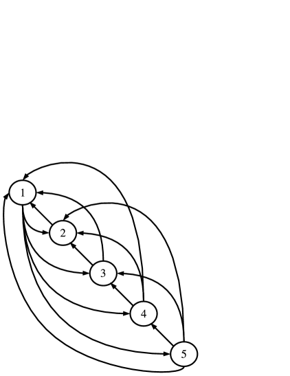
Figure 2. Dictatorial network on $5$ vertices.

If we apply Procedure Initial-Solution to the dictatorial networks in Figure 2, we obtain $U=\{1,2,3,4,5\}$ and $U^{\prime}=\emptyset$. Procedure Optimization returns $U=\{1\}$ and $U^{\prime}=\{2,3,4,5\}$. Finally, Procedure Nested gives $d=4$ and $U_{1}:=\{1\}\subset U_{2}:=\{1,5\}\subset U_{3}:=\{1,4,5\}\subset U_{4}:=\{1,3,4,5\}\subset U_{5}:=\{1,2,3,4,5\}=V$. In general, since the dictatorial network on $n$ vertices is such that

$$\partial\{1\} = \{n\}$$

$$\partial\{1,n\} = \{n-1\}$$

$$\partial\{1,n-1,n\} = \{n-2\}$$

$$\vdots$$

$$\partial\{1,3,\ldots,n\} = \{2\},$$

then algorithm Dominant–Vertices returns $d=n-1$ and $U_{1}=\{1\}\subset U_{2}=\{1,n\}\subset U_{3}=\{1,n-1,n\}\dots\subset U_{n}=V$. Of course, the dominant set that is produced by the algorithm is of minimal cardinality.

4.1.3. Democratic Networks

In contrast to the previous family of examples, here we present a collection of networks on $2n$ vertices, whose dominant sets have cardinality of at least $n$. They are bi–directional circuits on an even number of vertices, which we define as follows. The vertex set is $V:=\{0,2,\ldots,2n-1\}$, and arrows $A:=\{(u,v)\in V\times V:\ u-v\equiv 1(\mod 2n)\ \text{ or }u-v\equiv 2n-1(\mod 2n)\}$. The corresponding adjacency matrix has the form

$$M_{A}:=\left(\begin{matrix}0&1&0&0&\dots&0&0&1\\ 1&0&1&0&\dots&0&0&0\\ 0&1&0&1&\dots&0&0&0\\ 0&0&1&0&\dots&0&0&0\\ \vdots&&&&&&&\vdots\\ 0&0&0&0&\dots&1&0&1\\ 1&0&0&0&\dots&0&1&0\\ \end{matrix}\right).$$

We will refer to the network just defined as the democratic network on $2n$ vertices.

Figure 3 shows the democratic network on $6$ vertices, the set $\{0,3,4\}$ determines $\{1,3,5\}$, and vice versa.

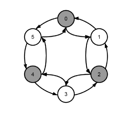
Figure 3. Democratic network on $6$ vertices.

Applying Procedure Initial-Solution to the democratic networks in Figure 3, we obtain $U=\{0,1,2,3,4\}$ and $U^{\prime}=\emptyset$. Procedure Optimization returns $U=\{0,2,4\}$ and $U^{\prime}=\{1,3,5\}$. Finally, Procedure Nested gives $d=1$ and $U_{1}:=\{0,2,4\}\subset U_{2}:=\{0,1,2,3,4,5\}=V$. In general, algorithm Dominant–Vertices returns $d=1$ and $U_{1}=\{0,2,4,\ldots,2n-2\}\subset U_{2}=\{0,1,2,3,\ldots,2n-1\}=V$. This is because

$$\partial\{0,2,4,6,\ldots,2n-2\} = \{1,3,5,\ldots,2n-1\}$$

$$\partial\{1,3,5\ldots,2n-1\} = \{0,2,4,6,\ldots,2n-2\}.$$

Notice that the dominant set that is produced by the algorithm is of minimal cardinality.

In the three examples examined so far, the dominant set $U$ determined by the Algorithm Dominant–Vertices is of minimal cardinality, and the complement $U^{\prime}=V\setminus U$ is dominant as well, but this is not the general case. Furthermore, even when $U^{\prime}=V\setminus U$ is dominant, the number of steps needed to determine $U$ from $U^{\prime}$ can be different from the number $d$ given by the algorithm. This is in particular the case of the dictatorial networks.

4.2. Inhering Dominance

To illustrate how dominance is inherited to subnetworks, we will consider three supergraphs of the dictatorial network in Figure 2, which we present in Figure 4. Starting with the network at left, we obtained the other two by eliminating an increasing number of arrows, keeping a strongly connected network each time. For the graph at left, $\{1,2,3\}$ is the dominant set of vertices given by the Algorithm Dominant–Vertices. Applying the same algorithm to the network at the center of the figure, we obtain $\{1,2\}$ as the dominant set. Finally, for the dictatorial network on $5$ vertices, vertex number $1$ is the dominant vertex the algorithm returns.

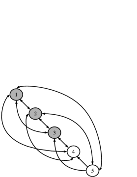
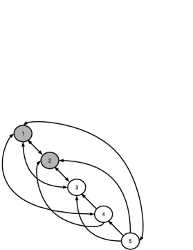
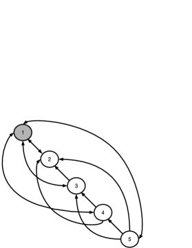
Figure 4. Supernetworks of the dictatorial network on $5$ vertices. Their respective dominant vertices are colored in gray.

5. Numerical Examples

In this section we consider two families of random networks, and we determine a dominant set of vertices by means of the Algorithm Dominant–Vertices. We will characterize the structural complexity of the network through the expected size of the dominant set $U$ and the number of steps $d$ needed to determine $V$ from $U$.

5.1. Erdos̈–Rényi networks

An Erdos̈–Rényi digraph is constructed as follows. Fix a set of vertices $V$ and $p\in(0,1]$. The arrow set $A\subseteq V\times V$ is such that for each $u,v\in V$, $\mathbb{P}\{(u,v)\in A\}=p$. According to this, a given arrow $(u,v)$ belongs to the digraph with probability $p$, and the inclusion of different vertices are independent and identically distributed random variables (for more details on random graphs and their dynamical construction see [5] for instance).

For $p=0.1,0.2,\ldots,1$ and $\#V=50,100,200$, we have generated 100 Erdos̈–Rényi digraphs, and for each one of those 3000 networks, we have computed a dominant set of vertices $U$ and a depth $d$, by using Algorithm Dominant–Vertices. On top of Figure 5 we show the expected number of dominant vertices $\mathbb{E}(\#U)$ the Algorithm Dominant–Vertices returns, and in error bars the size of the fluctuations $s(\#U):=\sqrt{\mathbb{E}(\#U-\mathbb{E}(\#U))^{2}}$, both as a function of $p$, and for the three scenarios $\#V=50,100,200$. In the lower frame of the same figure we plot the expected number of steps $\mathbb{E}(d)$ given by the same algorithm, with error bars proportional to the corresponding standard deviation $s(d):=\sqrt{\mathbb{E}(d-\mathbb{E}(d))^{2}}$, both as a function of the connection probability $p$.

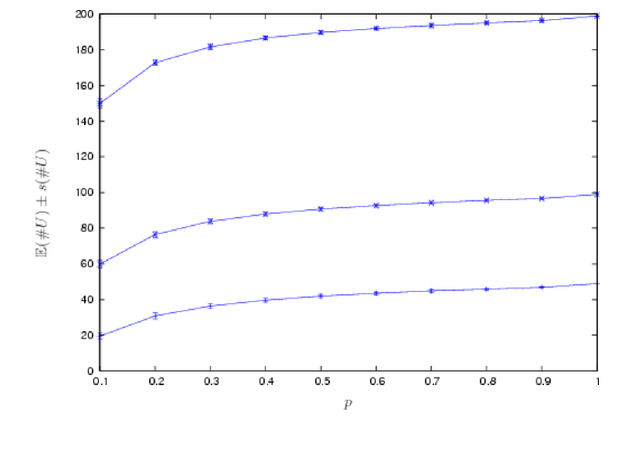
Figure 5. On top, the expected number of dominant vertices $\mathbb{E}(\#U)$, with error bars corresponding to the fluctuation $s(\#U):=\sqrt{\mathbb{E}(\#U-\mathbb{E}(\#U))^{2}}$, both as a function of $p$. On bottom, the mean depth $\mathbb{E}(d)$, with error bars proportional to the corresponding standard deviation $s(d):=\sqrt{\mathbb{E}(d-\mathbb{E}(d))^{2}}$, both as a function of the connection probability $p$. In both frames we compare the three scenarios $\#V=50,100$ and $200$, and their corresponding curves appeared ordered from bottom to top.

In Figure 6 we show a realization of an Erdos̈–Rényi network on $100$ vertices, with probability of connection $p=0.1$. For this example, the Algorithm Dominant–Vertices retunrs $\#U=58$ and $d=13$.

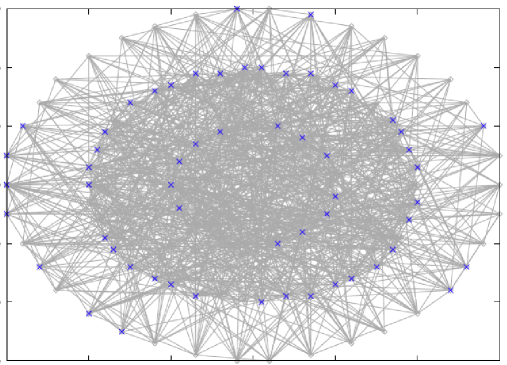
Figure 6. Realization of an Erdos̈–Rényi Network on 100 vertices. The dominant vertices determined by the Algorithm Dominant–Vertices are marked with a $\times$.

For the completely connected network on $N$ vertices, any dominant set has cardinality $N-1$ and depth $d=1$. Our numerical results show how the Erdos̈–Rényi networks approaches this situation as the probability of connection goes to 1. More specifically, as $p\to 1$, the size of the dominant set $\mathbb{E}(\#U)\to N$, while $\mathbb{E}(d)\to 1$.

5.2. Barabási–Albert Networks

We implemented a dynamical construction of scale–free graphs similar to the one proposed by Barabási and Albert. We start, at $n=0$, with a kernel graph $\mathcal{G}_{0}$, which is the complete simple graph on $m_{0}$ vertices. Then, for each $n\geqslant 1$, we add a new vertex $v_{n+1}$ to the preceding graph $\mathcal{G}_{n}:=(E_{n},V_{n})$. This new vertex form new edges with randomly chosen vertices in $V_{n}$. A given vertex $v\in V_{n}$ has probability proportional to its degree to be selected, and we have

$$\{v_{n+1},v\}\in E_{n}\text{ with probability }p_{n}(v):=\frac{\#\{u\in V_{n}:\ \{u,v\}\in E_{n}\}}{\#E_{n}}.$$

The graph at the $(n+1)$–th step is $\mathcal{G}_{n+1}$, with $V_{n+1}:=V_{n}\cup\{v_{n+1}\}$, and an enlarged edge set $E_{n+1}$. This random iteration continues until a predetermined number of vertices is obtained. In our dynamical construction it is possible to add several edge at each iteration, in opposition to the traditional scheme where only one edge is added at each time step. We finally assign directions to the edges in $E_{N-m_{0}}$, by choosing one of the two possible directions with probability $1/4$, and both directions with probability $1/2$ (for a rigorous study of scale–free and related random graphs, see [5]).

For $\#V=50,100,200$, and $m_{0}=0.06\times\#V,0.10\times\#V,0.14\times\#V,\ldots,0.38\times\#V$, we have generated 100 Barabási–Albert networks, and for each one of those 2700 digraphs, we have computed $U$ and $d$, by using Algorithm Dominant–Vertices. Figure 7 is the analogous to Figure 5 above. It shows in the upper frame the behavior of $\mathbb{E}(\#U)-m_{0}$, the expected number of dominant vertices exceeding the kernel of size, as a function of the relative size of the kernel $m_{0}/\#V$. In error bars we plot the size of the corresponding fluctuations $s(\#U):=\sqrt{\mathbb{E}(\#U-\mathbb{E}(\#U))^{2}}$. The frame at bottom shows the mean depth $\mathbb{E}(d)$ given by the same algorithm, and error bars proportional to the corresponding standard deviation $s(\#d):=\sqrt{\mathbb{E}(d-\mathbb{E}(d))^{2}}$, also as a function of the relative size of the kernel. In both frames we compare the three scenarios $\#V=50,100$ and $200$.

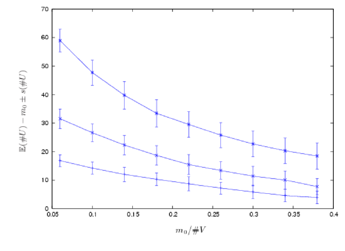
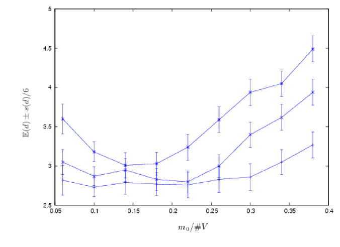
Figure 7. In top, the behavior of $\mathbb{E}(\#U)-m_{0}$ as a function of the relative size of the kernel $m_{0}/\#V$. The fluctuations $s(\#U):=\sqrt{\mathbb{E}(\#U-\mathbb{E}(\#U))^{2}}$ are indicated by the error bars. At bottom, the mean depth $\mathbb{E}(d)$, and error bars proportional to the corresponding standard deviation $s(\#d):=\sqrt{\mathbb{E}(d-\mathbb{E}(d))^{2}}$, both as functions of the relative size of the kernel. In both frames we compare the three scenarios $\#V=50,100$ and $200$, and their corresponding curves appeared ordered from bottom to top.

In Figure 8 we show a realization of a Barabási–Albert network on $100$ vertices, with kernel size $m_{0}=6$. For this example, the Algorithm Dominant–Vertices retunrs $\#U=37$ and $d=3$.

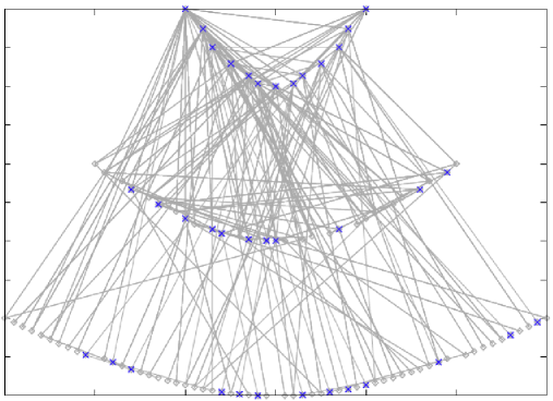
Figure 8. Realization of a Barabási–Albert Network on 100 vertices. The dominant vertices determined by the Algorithm Dominant–Vertices are marked with a $\times$.

We observed that the size of the dominant set for a Barabási–Albert network increases as the relative size of the kernel grows, in a similar way as in the Erdos̈–Rényi case. Nevertheless, there is an important difference. Since the kernel is build from a complete graph, the size of the dominant set is expected to be at least as large as the kernel. We observe that number extra vertices needed to complete the dominant set decreases with the size of the kernel. At the same time, the depth of the dominant set follows a non–monotonic behavior.

6. Final comments

Our definition of dominant vertices depends only on the structure of the underlying network, and for orbits (or forced trajectories) uniform separated from the discontinuity set, those vertices capture the dynamical state of the whole network. In the general case, for orbits accumulating at the discontinuity set, another definition of domination should be considered. Nevertheless, since uniform separation from the discontinuity set is typical, our algorithm determines observation (or control) nodes, in all but a negligible proportion of the cases.

One could interpret our main result as the existence of a effective network, smaller than the underlying network, which could be constructed from the dominant set of vertices. The dynamics on the effective network would be equivalent to the original one. Though such a network reduction can be attempted, specially in the case of $a=0$ (instantaneous degradation), the resulting dynamical system is not necessarily simpler that the original one.

The algorithm we propose is non–deterministic, and several alternative formulations can be considered. For instance, in the procedure Initial-Solution one chooses vertices with minimal input degree, amongst those of maximal output degree. Alternatively, one could choose vertices maximizing the output degree, amongst those of minimal input degree. We have considered this alternative, and we have found that in general it produces larger dominant sets. In spite of this, we expect that this algorithm can be improved, but that was not our aim in this work. Instead, we have tested the efficiency of the algorithm on examples where the dominant sets of vertices can be explicitly determined, and we have found optimal or almost optimal results.

Finally, the properties of dominant sets of vertices can be used to characterize the complexity of a given network. We have done this for the Erdos̈–Rényi and for the Barabási–Albert ensembles of random networks. This topological characterization has to be contrasted with a dynamical one, and this is what we intend to do in a future work.

References

- [1] M. Andrecut and S. A. Kauffman, “Mean-field model of genetic regulatory networks”, New Journal of Physics 8 (2006) 158–212.
- [2] R. Coutinho, B. Fernandez, R. Lima and A. Meyroneinc, “Discrete–time Piecewise Affine Models of Genetic RegulatoryNetworks”, Journal of Mathematical Biology 52 (4) (2006) 524–570.
- [3] A. Cros, A. Morante and E. Ugalde, “Regulatory Dynamics on Random Networks: Asymptotic Periodicity and Modularity”, submitted (2007). Available at http://lanl.arxiv.org/abs/0707.1551
- [4] H. de Jong, “Modeling and Simulation of Genetic Regulatory Systems: A Literature Review”, Journal of Computational Biology 9(1) (2002) 69–105.
- [5] R. Durret “Random Graph Dynamics” Cambridge Series in Statistical and Probabilistic Mathematics 20, Cambridge University Press 2007.
- [6] R. Edwards, “Analysis of Continuous–time Switching Networks”, Physica D 146 (2000) 165–199.
- [7] K. Glass and S. A. Kauffman “The Logical Analysis of Continuous, Nonlinear Biochemical Control Networks”, Journal of Theoretical Biology 44 (1974) 167-190.
- [8] T. Haynes, S. Hedetniemi and P. Slater, “Fundamentals of Domination in graphs”, CRC Press 1998.
- [9] S. A. Kauffman, “Metabolic Stability and Epigenesis in Randomly Constructed Genetic Nets”, Journal of Theoretical Biology 22 (1969) 437–467.
- [10] T. Mestl, E. Plathe, and S. W. Omholt, “A Mathematical Framework for Describing and Analyzing Gene Regulatory Networks”, Journal of Theoretical Biolology 176 (1995) 291–300.
- [11] R. Lima and E. Ugalde, “Dynamical Complexity of Discrete–time Regulatory Networks”, Nonlinearity 19 (1) (2006), 237–259.
- [12] M. E. J. Newman, “The structure and function of complex networks”, SIAM Review 45 (2003) 167–256.
- [13] D. Thieffry and R. Thomas, “Dynamical Behavior of Biological Networks”, Bulletin of Mathematical Biology 57 (2)(1995) 277–297.
- [14] D. Volchenkov and R. Lima, “Random Shuffling of Switching Parameters in a Model of Gene Expression Regulatory Network”, Stochastics and Dynamics 5 (1) (2005), 75–95.