De Sitter cosmology from Gauss-Bonnet dark energy with quantum effects

Abstract

A Gauss-Bonnet dark energy model is considered, which is inspired in string/M-theory and takes also into account quantum contributions. Those are introduced from a conformal quantum anomaly. The corresponding solutions for the Hubble rate, $H$, are studied starting from the Friedmann-Robertson-Walker equation. It is seen that, as a pure effect of the quantum contributions, a new solution for $H$ exists in some region, which does not appear in the classical case. The behavior of all encountered solutions is studied with care, in particular, the role played by the quantum correction term—which depends on the number of matter fields—on the stability of the solutions around its asymptotic value. It is argued that, contrary to what happens in the classical case, quantum effects remarkably lead to the realization of a de Sitter stage which corresponds to the inflation/dark energy stages, even for positive values of the $f_{0}$ constant (coupling of the field with the Gauss-Bonnet invariant).

I Introduction

One of the most intriguing questions in today’s Physics concerns the nature of the dark energy known to be present in the Universe we live in. The existence of such energy—with an almost uniform density distribution and a substantial negative pressure—which completely dominates all other forms of matter at present time, is inferred from several astronomical observations SuNv . In particular, according to recent astrophysical data analysis, this dark energy seems to behave very similarly to a cosmological constant, which is responsible for the accelerating expansion of the observable universe. Furthermore, there are strong reasons to believe that answering this question will have much to do with the possibility to explain the physics of the very early Universe.

Models of dark energy are abundant. One of the proposed candidates for it is the so-called phantom field, thus named because it corresponds to a negative-energy field. The peculiar properties of a phantom scalar (with negative kinetic energy) in a space with non-zero cosmological constant have been discussed in an interesting paper by Gibbons Gibbons . As indicated there, phantom properties bear some similarity with quantum effects phtmtr . An important property of the investigation in Gibbons is that it is easily generalizable to other constant-curvature spaces, such as Anti-de Sitter (AdS) space. Presently, there is considerable interest in such spaces, coming in particular from the AdS/CFT correspondence. According to it, the AdS space may have cosmological relevance cvetic , e.g. by increasing the number of particles created on a given subspace jcap . It could also be used to study a cosmological AdS/CFT correspondence b494 : the study of a phantom field in AdS space may give us hints about the origin of this field via the dual description. In the supergravity formulation one may think of the phantom as of a special renormalization group (RG) flow for scalars in gauged AdS supergravity. (Actually, such a RG flow may correspond to an imaginary scalar.)

Another candidate for dark energy is the tachyon EEQJ1 ; snsdo . This is an unstable field, actually. The interest of models exhibiting a tachyon is motivated by its role in the Dirac-Born-Infeld (DBI) action as a description of the D-brane action copeland ; s1 ; s2 . In spite of the fact that the tachyon represents an unstable field, its role in cosmology is generally still considered to be useful, as a source of dark matter snsdo ; Gibbons2 and, depending on the form of the associated potential Paddy ; Bagla ; AF ; AL ; GZ , it can actually lead to a period of inflation. On the other hand, it is important to realize that a tachyon with negative kinetic energy (yet another type of phantom) can also be introduced hao . In that phantom/tachyon model the thermodynamical parameter $w$ is naturally negative. In this case, the late-time de Sitter attractor solution is admissible, and this is one of the main reasons why it can be considered as an interesting model for dark energy hao . Moreover, in order to understand the role of the tachyon in cosmology it is necessary to study its effects on other backgrounds, as in the case of an Anti-de Sitter background EEQJ1 .

Another remarkable proposal is that the origin of the dark energy could in fact be related with the problem of the cosmological constant. One of the most interesting approaches to this paradigm is modified gravity. Actually, it is not absolutely clear why standard General Relativity should be trusted at large cosmological scales (thus, through an enormous range of orders of magnitude). One may assume that, considering minimal modifications, the gravitational action contains some additional terms growing slowly in the presence of decreasing curvature (see, e.g., capozziello ; NOPRD ; ln ; tr ; sasaki ; sami ; string and, for a review, see GB2 ), which could be responsible for the current acceleration. Within such scenario one of the most accepted approaches is the model of modified Gauss-Bonnet (GB) gravity. In this model additional terms in the gravitational action are introduced by means of a function which depends on the scalar curvature, $R$, and on the Gauss-Bonnet invariant, $G$ GB1 . It is possible to demonstrate that such models lead to a plausible effective cosmological constant, quintessence, or phantom eras. From these results one can conclude that, concerning its role as a gravitational alternative for DE, modified GB gravity may become a very strong candidate GB-gravity .

In the present paper we will consider a Gauss-Bonnet model for gravity, together with the first contributions coming from quantum effects. A stringy correction will be added to the ordinary General Relativity action, that is, a term proportional to the GB invariant $G$. We will duely take into account the quantum effects coming from matter, and their influence on the stability of the de Sitter universe will be carefully discussed.

II THE MODEL

We consider the model consisting of a scalar field, $\phi$, coupled with gravity in a rather non-trivial way and, as advanced, we will also take into account quantum effects.

As a stringy correction, the term proportional to the Gauss-Bonnet invariant, $G$, is written as:

$$G=R^{2}-4R_{\mu\nu}R^{\mu\nu}+R_{\mu\nu\rho\sigma}R^{\mu\nu\rho\sigma}\ .$$ (1)

The starting action is given by

$$S=\int d^{4}x\sqrt{-g}\left\{\frac{1}{2\kappa^{2}}R-\frac{\gamma}{2}\partial_{\mu}\phi\partial^{\mu}\phi-V(\phi)+f(\phi)G\right\}\ .$$ (2)

Here $\gamma=\pm 1$. Action (2) has been proposed as a stringy dark energy model in sasaki . It is interesting to note that one can also add to this system $R^{3}$ and $R^{4}$ stringy corrections sami ; sami1 (for a general introduction to modified gravity, see GB2 ; snsd1 ). Moreover, action (2) is able to solve the initial singularity problem ART ; nick For the canonical scalar, $\gamma=1$ and, at least when the GB term is not included, the scalar behaves as a phantom only when $\gamma=-1$ caldwell , showing in this case properties similar to those of a quantum field phtmtr . In analogy with the model in coupled —where also a non-trivial coupling of the scalar Lagrangian with some power of the curvature was considered—one may expect that a GB coupling term of this kind can be relevant for the explanation of the dark energy dominance nowadays.

Doing the same as in Ref. sasaki , by varying over $\phi$, one obtains

$$0=\gamma\nabla^{2}\phi-V^{\prime}(\phi)+f^{\prime}(\phi)G\ .$$ (3)

On the other hand, performing the variation over the metric $g_{\mu\nu}$ (as in gcsnsdosz ), gives

$$0 = \frac{1}{\kappa^{2}}\left(-R^{\mu\nu}+\frac{1}{2}g^{\mu\nu}R\right)+\gamma\left(\frac{1}{2}\partial^{\mu}\phi\partial^{\nu}\phi-\frac{1}{4}g^{\mu\nu}\partial_{\rho}\phi\partial^{\rho}\phi\right)+\frac{1}{2}g^{\mu\nu}\left(-V(\phi)+f(\phi)G\right)$$ (4)

$$-2f(\phi)RR^{\mu\nu}+2\nabla^{\mu}\nabla^{\nu}\left(f(\phi)R\right)-2g^{\mu\nu}\nabla^{2}\left(f(\phi)R\right)$$

$$+8f(\phi)R^{\mu}_{\ \rho}R^{\nu\rho}-4\nabla_{\rho}\nabla^{\mu}\left(f(\phi)R^{\nu\rho}\right)-4\nabla_{\rho}\nabla^{\nu}\left(f(\phi)R^{\mu\rho}\right)$$

$$+4\nabla^{2}\left(f(\phi)R^{\mu\nu}\right)+4g^{\mu\nu}\nabla_{\rho}\nabla_{\sigma}\left(f(\phi)R^{\rho\sigma}\right)-2f(\phi)R^{\mu\rho\sigma\tau}R^{\nu}_{\ \rho\sigma\tau}+4\nabla_{\rho}\nabla_{\sigma}\left(f(\phi)R^{\mu\rho\sigma\nu}\right)\,.$$

And using the identities obtained from the Bianchi identity,

$$\nabla^{\rho}R_{\rho\tau\mu\nu} = \nabla_{\mu}R_{\nu\tau}-\nabla_{\nu}R_{\mu\tau}\ ,$$

$$\nabla^{\rho}R_{\rho\mu} = \frac{1}{2}\nabla_{\mu}R\ ,$$

$$\nabla_{\rho}\nabla_{\sigma}R^{\mu\rho\nu\sigma} = \nabla^{2}R^{\mu\nu}-{1\over 2}\nabla^{\mu}\nabla^{\nu}R+R^{\mu\rho\nu\sigma}R_{\rho\sigma}-R^{\mu}_{\ \rho}R^{\nu\rho}\ ,$$

$$\nabla_{\rho}\nabla^{\mu}R^{\rho\nu}+\nabla_{\rho}\nabla^{\nu}R^{\rho\mu} = {1\over 2}\left(\nabla^{\mu}\nabla^{\nu}R+\nabla^{\nu}\nabla^{\mu}R\right)-2R^{\mu\rho\nu\sigma}R_{\rho\sigma}+2R^{\mu}_{\ \rho}R^{\nu\rho}\ ,$$

$$\nabla_{\rho}\nabla_{\sigma}R^{\rho\sigma} = {1\over 2}\Box R\ ,$$ (5)

one can rewrite (4) as

$$0 = \frac{1}{\kappa^{2}}\left(-R^{\mu\nu}+\frac{1}{2}g^{\mu\nu}R\right)+\gamma\left(\frac{1}{2}\partial^{\mu}\phi\partial^{\nu}\phi-\frac{1}{4}g^{\mu\nu}\partial_{\rho}\phi\partial^{\rho}\phi\right)+\frac{1}{2}g^{\mu\nu}\left(-V(\phi)+f(\phi)G\right)$$ (6)

$$-2f(\phi)RR^{\mu\nu}+4f(\phi)R^{\mu}_{\ \rho}R^{\nu\rho}-2f(\phi)R^{\mu\rho\sigma\tau}R^{\nu}_{\ \rho\sigma\tau}+4f(\phi)R^{\mu\rho\sigma\nu}R_{\rho\sigma}$$

$$+2\left(\nabla^{\mu}\nabla^{\nu}f(\phi)\right)R-2g^{\mu\nu}\left(\nabla^{2}f(\phi)\right)R-4\left(\nabla_{\rho}\nabla^{\mu}f(\phi)\right)R^{\nu\rho}-4\left(\nabla_{\rho}\nabla^{\nu}f(\phi)\right)R^{\mu\rho}$$

$$+4\left(\nabla^{2}f(\phi)\right)R^{\mu\nu}+4g^{\mu\nu}\left(\nabla_{\rho}\nabla_{\sigma}f(\phi)\right)R^{\rho\sigma}-4\left(\nabla_{\rho}\nabla_{\sigma}f(\phi)\right)R^{\mu\rho\nu\sigma}\ .$$

The above expression is valid in arbitrary spacetime dimensions. In four dimensions, the terms proportional to $f(\phi)$ without derivatives are canceled among themselves, and vanish, since the GB invariant is a total derivative in four dimensions.

Quantum effects can be included by taking into account the contribution of the conformal anomaly, $T_{A}$, defined as follows:

$$T_{A}=b\left(F+{2\over 3}\Box R\right)+b^{\prime}G+b^{\prime\prime}\Box R\ ,$$ (7)

where $F$ is the square of a 4d Weyl tensor and $G$ is the Gauss-Bonnet curvature invariant. They are given by

$$F = (1/3)R^{2}-2R_{ij}R^{ij}+R_{ijkl}R^{ijkl}\,,$$

$$G = R^{2}-4R_{ij}R^{ij}+R_{ijkl}R^{ijkl}\,.$$ (8)

In general, with $N$ scalar, $N_{1/2}$ spinor, $N_{1}$ vector fields, $N_{2}$ ($=0$ or $1$) gravitons, and $N_{\rm HD}$ higher-derivative conformal scalars, the coefficients $b$ and $b^{\prime}$ take the form

$$b={N+6N_{1/2}+12N_{1}+611N_{2}-8N_{\rm HD}\over 120(4\pi)^{2}}\,,$$

$$b^{\prime}=-{N+11N_{1/2}+62N_{1}+1411N_{2}-28N_{\rm HD}\over 360(4\pi)^{2}}\,.$$ (9)

We have that $b>0$ and $b^{\prime}<0$ for usual matter, except for higher derivative conformal scalars. Notice that $b^{\prime\prime}$ can be shifted by a finite renormalization of the local counterterm $R^{2}$, thus $b^{\prime\prime}$ can be arbitrary.

In terms of the corresponding energy density nojiri ; tsujikawa , $\rho_{A}$, and of the pressure density, $p_{A}$, $T_{A}$ is given by $T_{A}=-\rho_{A}+3p_{A}$. Using the energy conservation law in the Friedmann-Robertson-Walker (FRW) universe,

$$\dot{\rho}_{A}+3H\left(\rho_{A}+p_{A}\right)=0\,,$$ (10)

we can eliminate $p_{A}$, as

$$T_{A}=-4\rho_{A}-\dot{\rho}_{A}/H\,.$$ (11)

This yields the following expression for $\rho_{A}$:

$$\rho_{A} = -\frac{1}{a^{4}}\int{\rm d}t\,a^{4}HT_{A}$$ (12)

$$= -\frac{1}{a^{4}}\int{\rm d}t\,a^{4}H\Bigl{[}-12b\dot{H}^{2}+24b^{\prime}(-\dot{H}^{2}+H^{2}\dot{H}+H^{4})$$

$$-(4b+6b^{\prime\prime})\left(\dddot{H}+7H\ddot{H}+4\dot{H}^{2}+12H^{2}\dot{H}\right)\Bigr{]}\,.$$

Now, for the FRW universe metric,

$$ds^{2}=-dt^{2}+a(t)^{2}\sum_{i=1}^{3}\left(dx^{i}\right)^{2}\ ,$$ (13)

taking into account the contribution from the quantum anomaly, $T_{A}$, the equation of motion (4) becomes

$$0=-\frac{3}{\kappa^{2}}H^{2}+\frac{\gamma}{2}{\dot{\phi}}^{2}+V(\phi)-24\dot{\phi}f^{\prime}(\phi)H^{3}+\rho_{A}\ .$$ (14)

An equation of this sort (14) was also obtained for dilatonic gravity brevik99 ; quiroga7 . On the other hand, Eq. (2) becomes

$$0=-\gamma\left(\ddot{\phi}+3H\dot{\phi}\right)-V^{\prime}(\phi)+24f^{\prime}(\phi)\left(\dot{H}H^{2}+H^{4}\right)\ .$$ (15)

In the above equations it has been assumed that $\phi$ only depends on time.

Postulating the de Sitter solution, i.e. looking for solutions of the form $a=a_{0}\exp{(Ht)}$, where $H$ and the scalars are constant, we have for $\rho_{A}$ that

$$\rho_{A}=-6b^{\prime}H\,.$$ (16)

After this, Eq. (14) becomes

$$0=-\frac{3}{\kappa^{2}}H^{2}+V(\phi)-6b^{\prime}H\ .$$ (17)

And, since we are looking for solutions with $H=$ const, we are now interested in solving the equations of motion in the form

$$-V^{\prime}(\phi)+24f^{\prime}(\phi)(\dot{H}H^{2}+H^{4}) = 0\,,$$ (18)

$$-\frac{3}{\kappa^{2}}H^{2}+V(\phi)-6b^{\prime}H = 0\,.$$ (19)

We may now consider the case when $V(\phi)$ and $f(\phi)$ are given as exponents, with some constant parameters $V_{0}\,,f_{0}\,\mbox{and}\,\phi_{0}$,

$$V=V_{0}\ {\rm e}^{-\frac{2\phi}{\phi_{0}}}\ ,\quad f(\phi)=f_{0}\ {\rm e}^{\frac{2\phi}{\phi_{0}}}\,,$$ (20)

these are string-inspired values for the potentials. Assuming the scale factor to behave as $a=a_{0}\exp{(Ht)}$, we get the following equations of motion

$$\frac{2}{\phi_{0}}V_{0}{{\rm e}^{-\frac{2\phi}{\phi_{0}}}}+48\left(\frac{f_{0}}{\phi_{0}}\right){\rm e}^{\frac{2\phi}{\phi_{0}}}H^{4} = 0\,,$$ (21)

$$-\frac{3}{\kappa^{2}}H^{2}+V_{0}{\rm e}^{-\frac{2\phi}{\phi_{0}}}-6b^{\prime}H = 0\,.$$ (22)

Now, combining Eqs. (21) and (22) we find the following equation for $H$:

$$H^{3}+\left(\frac{{\rm e}^{-\frac{2\phi}{\phi_{0}}}}{8f_{0}\kappa^{2}}\right)H+\frac{b^{\prime}}{4f_{0}}{\rm e}^{-\frac{2\phi}{\phi_{0}}}=0\,.$$ (23)

If we switch off the quantum effects ($b^{\prime}=0$), then we find for $H^{2}$:

$$H^{2}=-\frac{V}{8V_{0}f_{0}\kappa^{2}}\,.$$ (24)

This is the pure classical solution, which was obtained in sasaki . This solution may require the coupling $f_{0}$ to be negative, otherwise the solution may not exist. Furthermore, since the Hubble rate can be determined by the initial condition ($H=H_{0}$), the choice of $\phi_{0}$ is fully arbitrary.

Returning to Eq. (23), in looking for a solution which takes into account quantum effects, we easily find a numerical one by rewriting Eq. (23) in terms of the potential $V$, as follows,

$$H^{3}+\frac{V}{8f_{0}V_{0}\kappa^{2}}H+\frac{b^{\prime}V}{4V_{0}f_{0}}=0\,.$$ (25)

This equation has the form of a reduced cubic equation and thus it is possible to find a solution by using Cartan’s formula. The discriminant of the cubic equation is

$$D=\frac{V^{3}}{(24)^{3}f_{0}^{3}V_{0}^{3}\kappa^{6}}\left(1+\frac{216b^{\prime 2}f_{0}V_{0}\kappa^{6}}{V}\right)\,.$$ (26)

As seen from (26), for the cubic equation (23) the sign of the discriminant depends on the sign of $f_{0}$, since we define $V_{0}$ to be positive.

For the analysis of the solutions of Eq. (25) in this case, we will better consider numerical solutions and look for the behavior of the Hubble rate $H$ as a function of the potential $V$. Let us consider, as a first case, the solution with the following values for the parameters: $f_{0}=-0.5,\ V_{0}=1,\ b^{\prime}=-0.5$, and $\kappa=16\pi G$, where $G=6.63\times 10^{-8}$ is the gravitational constant. For those, the behavior of $H$ is illustrated in Fig. 1.

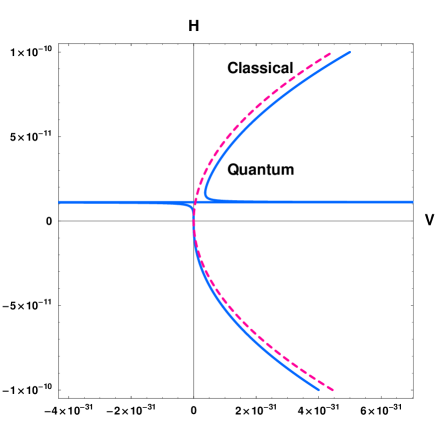
Figure 1: Behavior of the Hubble rate $H$ as a function of the potential $V$, for several values of $V$.

We immediately see from this figure that we indeed have three possible ways to define $H$ as a function of the potential $V$. That is, of course, a consequence of the three possible solutions of the cubic equation (25). We will be interested only in the case when $H$ has positive values for positive values of the potential $V$.

As seen in the plot, the Hubble rate $H$ is growing as the potential grows, starting from some minimal positive value. From another side, it is important to remark that there is a positive solution for $H$ which is very close to the classical solution (dashed line), up to the point where the continuous-line solution tends asymptotically to a very small value. This case clearly shows that quantum effects are only a perturbation to the classical solution. It is also clear from Fig. 1 the interesting feature that the asymptotic value of $H$ depends on the quantum correction term $b^{\prime}$, which on its turn depends on the number of fields $N$. This means that the asymptotic value attains a greater positive value if $N$ is larger. In the absence of the $b^{\prime}$ term this discontinuous behavior of the solution for $H$ disappears. This leads to the conclusion that the instability of the solution around its asymptotic value is exclusively due to quantum effects.

It is remarkable that there exists, owing to the quantum effects, another possible solution for $H$ with a positive value for $f_{0}$. This solution exists in a very small region, as a pure effect of quantum contributions since it turns out that in the classical case sasaki it is not possible to obtain any positive solutions for $H$—as seen from Eq. (24). In Fig. 2 the situation we have just discussed is shown, corresponding to a positive value for $f_{0}$.

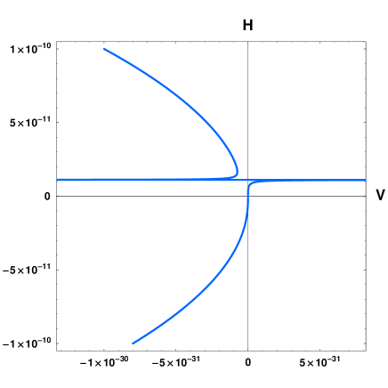
Figure 2: Behavior of the Hubble rate $H$ for several values of $V$, with a positive coupling of the scalar field with the Gauss-Bonnet invariant: $f_{0}>0$.

III CONCLUSIONS

To summarize, a number of quite interesting conclusions can be drawn from the present study of the influence of a combination of quantum effects and modified gravity as a possible way for interpreting dark energy in an accelerated inflationary de Sitter universe. In particular, it is expected that for large values of the curvature ($R=6\dot{H}+12H^{2}$) the de Sitter epoch thus described corresponds to early-time inflation.

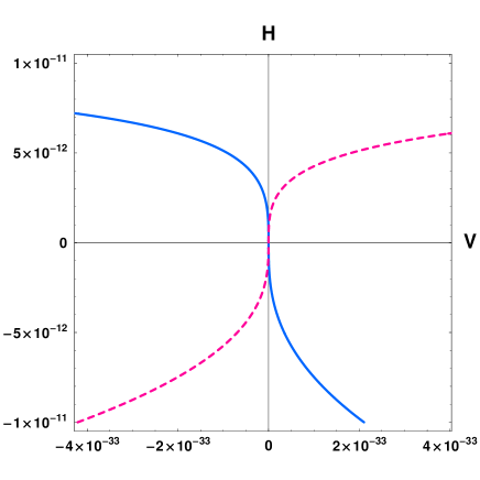
Figure 3: Behavior of the Hubble rate $H$ near its value at the dark energy stage. The dashed line corresponds to the positive coupling case, $f_{0}>0$, and the continuous line to the negative case, $f_{0}<0$.

From another point of view, for small values of curvature [$R\sim(10^{-33}$eV$)^{2}$] we expect that the de Sitter era realized in this model will correspond to the dark energy stage. However, as seen in Fig. 3, this occurs for both positive and negative values of the potential, depending on the sign of $f_{0}$. This result clearly shows that, contrary to what happens in the classical case, quantum effects lead in fact to the realization of the de Sitter era corresponding to the dark energy stage, even for positive values of the $f_{0}$ constant. Such situation may potentially have interesting cosmological consequences.

In a similar fashion, the coupling of GB dark energy with $F(R)$ gravity could be considered, too. This should not represent a big problem, in principle, owing to the fact that the curvature is constant on the solutions. That possibility deserves further investigation.

Acknowledgments

We are grateful to S.D. Odintsov for very helpful discussions. The research of JQH and HIA has been supported by Grants-in-Aid for Scientific Research, No 3-07-05 at the Universidad Tecnológica de Pereira, Colombia. The research of EE was partly done while on leave at the Department of Physics & Astronomy, Dartmouth College, 6127 Wilder Laboratory, Hanover, NH 03755, USA. EE was supported in part by MEC (Spain), project PR2006-02842, and by AGAUR (Generalitat de Catalunya), grant 2007BE-1003 and contract 2005SGR-00790.

References

- (1) S. Perlmutter et al., Astrophys. J. 517, 565 (1999); A. Riess et al., Astron. J. 116, 1009 (1998).
- (2) G. Gibbons, hep-th/0302199.
- (3) S. Nojiri and S.D. Odintsov, Phys. Lett. B562, 147 (2003), hep-th/0303117.
- (4) M. Cvetic, S. Nojiri and S.D. Odintsov, Phys. Rev. D69, 023513 (2004), hep-th/0306031.
- (5) S. Nojiri and S.D. Odintsov, JCAP 06, 004 (2003), hep-th/0303011.
- (6) S. Nojiri and S.D. Odintsov, Phys. Lett. B494, 135 (2000), hep-th/0008160.
- (7) E. Elizalde and J. Quiroga Hurtado, Int. J. Mod. Phys. D 14, 1439 (2005), gr-qc/0412106.
- (8) S. Nojiri and S.D. Odintsov, Phys. Lett. B571, 1 (2003), hep-th/0306212.
- (9) E.J. Copeland, M.R. Garousi, M. Sami, S. Tsujikawa, Phys. Rev. D 71, 043003 (2005), hep-th/0411192.
- (10) A. Sen, JHEP 0204, 048 (2002); JHEP 0207, 065 (2002); Mod. Phys. Lett. A17, 1797 (2002); Physica Scripta T 117, 70 (2005), hep-th/0312153.
- (11) A. Sen, JHEP 9910, 008 (1999); M.R. Garousi, Nucl. Phys. B584, 284 (2000); Nucl. Phys. B 647, 117 (2002); JHEP 0305, 058 (2003); E.A. Bergshoeff, M. de Roo, T.C. de Wit, E. Eyras, S. Panda, JHEP 0005, 009 (2000); J. Kluson, Phys. Rev. D 62, 126003 (2000); D. Kutasov and V. Niarchos, Nucl. Phys. B 666, 56 (2003).
- (12) G.W. Gibbons, Phys. Lett. B 537, 1 (2002); M. Fairbairn and M.H.G. Tytgat, Phys. Lett. B 546, 1 (2002); A. Feinstein, Phys. Rev. D 66, 063511 (2002); S. Mukohyama, Phys. Rev. D 66, 024009 (2002); D. Choudhury, D. Ghoshal, D.P. Jatkar and S. Panda, Phys. Lett. B 544, 231 (2002); G. Shiu and I. Wasserman, Phys. Lett. B 541, 6 (2002); L. Kofman and A. Linde, JHEP 0207, 004 (2002); M. Sami, Mod. Phys. Lett. A 18, 691 (2003); A. Mazumdar, S. Panda and A. Perez-Lorenzana, Nucl. Phys. B 614, 101 (2001); J.C. Hwang and H. Noh, Phys. Rev. D 66, 084009 (2002); Y.S. Piao, R.G. Cai, X.M. Zhang and Y.Z. Zhang, Phys. Rev. D 66, 121301 (2002); J.M. Cline, H. Firouzjahi and P. Martineau, JHEP 0211, 041 (2002); G.N. Felder, L. Kofman and A. Starobinsky, JHEP 0209, 026 (2002); S. Mukohyama, Phys. Rev. D 66, 123512 (2002); M.C. Bento, O. Bertolami and A.A. Sen, Phys. Rev. D 67, 063511 (2003); J.G. Hao and X.Z. Li, Phys. Rev. D 66, 087301 (2002); C.J. Kim, H.B. Kim and Y.B. Kim, Phys. Lett. B 552, 111 (2003); T. Matsuda, Phys. Rev. D 67, 083519 (2003); A. Das and A. DeBenedictis, Gen. Rel. Grav. 36, 1741 (2004), gr-qc/0304017; Z.K. Guo, Y.S. Piao, R.G. Cai and Y.Z. Zhang, Phys. Rev. D 68, 043508 (2003); G.W. Gibbons, Class. Quant. Grav. 20, S321 (2003); M. Majumdar and A.C. Davis, Phys. Rev. D 69, 103504 (2004), hep-th/0304226; E. Elizalde, J.E. Lidsey, S. Nojiri and S.D. Odintsov, Phys. Lett. B 574, 1 (2003), hep-th/0307177; D.A. Steer and F. Vernizzi, Phys. Rev. D 70, 043527 (2004); V. Gorini, U. Moschella and V. Pasquier, Phys. Rev. D 69, 123512 (2004); L.P. Chimento, Phys. Rev. D 69, 123517 (2004); M.B. Causse, astro-ph/0312206; B.C. Paul and M. Sami, Phys. Rev. D 70, 027301 (2004); G. N. Felder and L. Kofman, Phys. Rev. D 70, 046004 (2004); J.M. Aguirregabiria and R. Lazkoz, Mod. Phys. Lett. A 19, 927 (2004); L.R. Abramo, F. Finelli and T.S. Pereira, Phys. Rev. D 70, 063517 (2004), astro-ph/0405041; G. Calcagni, Phys. Rev. D 70, 103528 (2004), hep-th/0406006; J. Raeymaekers, JHEP 0410, 057 (2004); G. Calcagni and S. Tsujikawa, Phys. Rev. D 70, 103514 (2004), astro-ph/0407543; S.K. Srivastava, gr-qc/0409074; N. Barnaby and J.M. Cline, Int. J. Mod. Phys. A 19, 5455 (2004), hep-th/0410030.
- (13) T. Padmanabhan, Phys. Rev. D 66, 021301 (2002).
- (14) J. S. Bagla, H. K. Jassal and T. Padmanabhan, Phys. Rev. D 67, 063504 (2003).
- (15) L.R.W. Abramo and F. Finelli, Phys. Lett. B 575, 165 (2003).
- (16) J.M. Aguirregabiria and R. Lazkoz, Phys. Rev. D 69, 123502 (2004).
- (17) Z.K. Guo and Y.Z. Zhang, JCAP 0408, 010 (2004).
- (18) J.-G. Hao and X.-Z. Li, Phys. Rev. D68, 043501 (2003), hep-th/0305207; Phys. Rev. D68, 083514 (2003), hep-th/0306033.
- (19) S. Capozziello, Int. J. Mod. Phys. D 11, 483 (2002); S. Capozziello, S. Carloni and A. Troisi, astro-ph/0303041; S.M. Carroll, V. Duvvuri, M. Trodden and M.S. Turner, Phys. Rev. D 70, 043528 (2004), astro-ph/0306438.
- (20) S. Nojiri and S.D. Odintsov, Phys. Rev. D 68, 123512 (2003), hep-th/0307288.
- (21) S. Nojiri and S.D. Odintsov, Gen. Rel. Grav. 36, 1765 (2004), hep-th/0308176; S. Nojiri and S.D. Odintsov, hep-th/0608008; S. Capozziello, S. Nojiri, S.D. Odintsov and A. Troisi, Phys. Lett. B639, 135 (2006), astro-ph/0604431; X. Meng and P. Wang, Phys. Lett. B 584, 1 (2004), hep-th/0309062.
- (22) D. Easson, F. Schuller, M. Trodden and M. Wohlfarth, Phys. Rev. D 72, 043504 (2005), astro-ph/0506392.
- (23) S. Nojiri, S.D. Odintsov and M. Sasaki, Phys. Rev. D71, 2005, 123509, hep-th/0504052.
- (24) S. Nojiri, S.D. Odintsov and M. Sami, Phys. Rev. D74, 2006, 0460004, hep-th/0605039.
- (25) M. Sami, A. Toporensky, P. Trejakov and S. Tsujikawa, Phys. Lett. B619, 193 (2005), hep-th/0504154; G. Calcagni, S. Tsujikawa and M. Sami, Class. Quant. Grav. 22, 3977 (2005), hep-th/0505193; B.M.N. Carter and I. P. Neupane, Phys. Lett. B638, 94 (2006), hep-th/0510109.
- (26) S. Nojiri and S.D. Odintsov, hep-th/0601213.
- (27) S. Nojiri and S.D. Odintsov, Phys. Lett. B631,1 (2005), hep-th/0508049; S. Nojiri, S.D. Odintsov and O. Gorbunova, J. Phys. A 39, 6627 (2006), hep-th/0510183.
- (28) G. Cognola, E. Elizalde, S. Nojiri, S.D. Odintsov and S. Zerbini, Phys. Rev. D75, 086002 (2007)), hep-th/0611198.
- (29) E. Elizalde, S. Jhingan, S. Nojiri, S.D. Odintsov, M. Samiand and I. Thomgkool, ArXiv/0705.1211[hep-th]
- (30) S. Nojiri, S.D. Odintsov, hep-th/0611071.
- (31) I. Antoniadis, J. Rizos, K. Tamvakis, Nucl. Phys. B 415, 497 (1994) arXiv:hep-th/9305025; P. Kanti, J. Rizos and K. Tamvakis, Phys. Rev. D 59, 083512 (1999) arXiv:gr-qc/9806085.
- (32) N.E. Mavromatos and J. Rizos, Phys. Rev. D 62, 124004 (2000) arXiv:hep-th/0008074 ; JHEP 0207, 045 (2002) arXiv:hep-th/0205099 ; Int. J. Mod. Phys. A 18, 57 (2003) arXiv:hep-th/0205299.
- (33) R. Caldwell, Phys. Lett. B 545, 23 (2002) arXiv:astro-ph/9908168.
- (34) S. Nojiri and S.D. Odintsov, Phys. Lett. B 599, 137 (2004) arXiv:astro-ph/0403622 .
- (35) G. Cognola, E. Elizalde, S. Nojiri, S.D. Odintsov and S. Zerbini, Phys. Rev. D 73, 084007 (2006) hep-th/0601008.
- (36) S. Nojiri and S.D. Odintsov, Phys. Lett. B 595, 1 (2004) arXiv:hep-th/0405078 ; Phys. Rev. D 70, 103522 (2004) arXiv:hep-th/0408170 ; E. Elizalde, S. Nojiri and S.D. Odintsov, Phys. Rev. D 70, 043539 (2004) arXiv:hep-th/0405034 .
- (37) S. Nojiri, S.D. Odintsov and S. Tsujikawa, Phys. Rev. D 71, 063004 (2005) arXiv:hep-th/0501025.
- (38) I. Brevik and S.D. Odintsov, Phys. Lett. B 455, 104 (1999), hep-th/9902184.
- (39) I. Brevik and J. Quiroga Hurtado, Gen. Rel. Grav. 36, 1431 (2004), gr-qc/0311041.