Experimental Falsification of Leggett’s Non-Local Variable Model

Abstract

Bell’s theorem guarantees that no model based on local variables can reproduce quantum correlations. Also some models based on non-local variables, if subject to apparently “reasonable” constraints, may fail to reproduce quantum physics. In this paper, we introduce a family of inequalities, which allow testing Leggett’s non-local model versus quantum physics, and which can be tested in an experiment without additional assumptions. Our experimental data falsify Leggett’s model and are in agreement with quantum predictions.

Introduction. Quantum physics provides a precise rule to compute the probability that the measurement of $A$ and $B$ performed on two physical systems in the state $|\Psi\rangle$ will lead to the outcomes $(r_{A},r_{B})$:

$$P_{Q}(r_{A},r_{B}|A,B) = \langle\Psi|{\cal P}_{r_{A}}\otimes{\cal P}_{r_{B}}|\Psi\rangle$$ (1)

where ${\cal P}_{r}$ is the projector on the subspace associated to the measurement result $r$. For entangled states, this formula predicts that the outcomes are correlated, irrespective of the distance between the two measurement devices. A natural explanation for correlations established at a distance is pre-established agreement: the two particles have left the source with some common information $\lambda$, called a local variable (LV), that allows them to compute the outcomes for each possible measurement; formally, $r_{A}=f_{A}(A,\lambda)$ and $r_{B}=f_{B}(B,\lambda)$. Satisfactory as it may seem a priori, this model fails to reproduce all quantum correlations: this is the celebrated result of John Bell bell , by now tested in a very large number of experiments. The fact that quantum correlations can be attributed neither to LV nor to communication below the speed of light is referred to as quantum non-locality.

While non-locality is a striking manifestation of quantum entanglement, it is not yet clear how fundamental this notion really is: the essence of quantum physics may be somewhere else pr94 . For instance, non-determinism is another important feature of quantum physics, with no a priori link with non-locality. Generic theories featuring both non-determinism and non-locality have been studied, with several interesting achievements nlnd ; but it is not yet clear what singles quantum physics out. In order to progress in this direction, it is important to learn which other alternative models are compatible with quantum physics, which are not. Bell’s theorem having ruled out all possible LV models, we have to move on to models based on non-local variables (NLV). The first example of testable NLV model was the one by Suarez and Scarani sua97 , falsified in a series of experiments a few years ago zbi01 . A different such model was proposed more recently by Leggett leg03 . This model supposes that the source emits product quantum states $\mbox{$|\alpha\rangle$}\otimes\mbox{$|\beta\rangle$}$ with probability density $\rho(\alpha,\beta)$, and enforces that the marginal probabilities must be compatible with such states:

$$P(r_{A}|A) = \int d\rho(\alpha,\beta)\mbox{$\langle\alpha|{\cal P}_{r_{A}}|\alpha\rangle$}\,,$$ (2)

$$P(r_{B}|B) = \int d\rho(\alpha,\beta)\mbox{$\langle\beta|{\cal P}_{r_{B}}|\beta\rangle$}\,.$$ (3)

The correlations however must include some non-local effect, otherwise this would be a (non-deterministic) LV model and would already be ruled out by Bell’s theorem. What Leggett showed is that the simple requirement of consistency (i.e., no negative probabilities should appear at any stage) constrains the possible correlations, even non-local ones, to satisfy inequalities that are slightly but clearly violated by quantum physics. A recent experiment gro07 demonstrated that state-of-the-art setups can detect this violation in principle. However, their falsification of the Leggett model is flawed by the need for additional assumptions, because the inequality they used suppl , just as the original one by Leggett, supposes that data are collected from infinitely many measurement settings. In this paper, we present a family of inequalities, which allow testing Leggett’s model against quantum physics with a finite number of measurements. We show their experimental violation by pairs of polarization-entangled photons. We conclude with an overview of what has been learned and what is still to be learned about NLV models.

Theory. We restrict our theory to the case where the quantum degree of freedom under study is a qubit. We consider von Neumann measurements, that can be labeled by unit vectors in the Poincaré sphere $\mathcal{S}$: $A\rightarrow\vec{a}$ and $B\rightarrow\vec{b}$; their outcomes will be written $r_{A},r_{B}\in\{+1,-1\}$. Pure states of single particles can also be labeled by unit vectors $\vec{u},\vec{v}$ in $\mathcal{S}$. Leggett’s model requires

$$P(r_{A},r_{B}|\vec{a},\vec{b}) = \int d\rho(\vec{u},\vec{v})P_{\vec{u},\vec{v}}(r_{A},r_{B}|\vec{a},\vec{b})$$ (4)

with

$$P_{\vec{u},\vec{v}}(r_{A},r_{B}|\vec{a},\vec{b}) = \frac{1}{4}\Big{[}1+r_{A}\vec{a}\cdot\vec{u}+r_{B}\vec{b}\cdot\vec{v}$$ (5)

$$+r_{A}r_{B}C(\vec{u},\vec{v},\vec{a},\vec{b})\Big{]}\,.$$

The correlation coefficient $C(\vec{u},\vec{v},\vec{a},\vec{b})$ is constrained only by the requirement that (5) must define a probability distribution over $(r_{A},r_{B})$ for all choice of the measurements $\vec{a},\vec{b}$. Remarkably, this constraint is sufficient to derive inequalities that can be violated by quantum physics leg03 . The inequality derived in suppl (see also par07 for a subsequent shorter derivation) reads

$$\left|E_{1}(\varphi)+E_{1}(0)\right|+\left|E_{2}(\varphi)+E_{2}(0)\right| \leq 4-\frac{4}{\pi}\left|\sin\frac{\varphi}{2}\right|$$ (6)

where the quantities $E_{j}(\theta)$ are defined from the correlation coefficients

$$C(\vec{a},\vec{b}) = \sum_{r_{A},r_{B}}r_{A}r_{B}P(r_{A},r_{B}|\vec{a},\vec{b})$$ (7)

as follows. The index $j$ refers to a plane $\{\vec{a}\in\mathcal{S}|\vec{a}\cdot\vec{n}_{j}\ =0\}$ in the Poincaré sphere (for $\vec{n}_{j}\in\mathcal{S}$), and the two planes $j=1,2$ that appear in (6) must be orthogonal (i.e. $\vec{n}_{1}\cdot\vec{n}_{2}=0$). For each unit vector $\vec{a}_{j}$ of plane $j$, let’s define $\vec{a}_{j}^{\,\perp}=\vec{n}_{j}\times\vec{a}_{j}$. $E_{j}(\theta)$ is then the average of $C(\vec{a}_{j},\vec{b}_{j})$ over all directions $\vec{a}_{j}$, with $\vec{b}_{j}=\cos\theta\,\vec{a}_{j}+\sin\theta\,\vec{a}_{j}^{\,\perp}$ . This is a problematic feature of inequality (6): it can be checked only by performing an infinite number of measurements or by adding the assumption of rotational invariance of the correlation coefficients $C(\vec{a},\vec{b})$, as in gro07 . It is thus natural to try and replace the average over all possible settings with an average on a discrete set. This is done by the following estimate. Let $\vec{w}$ and $\vec{c}$ be two unit vectors, and let $R_{N}$ be the rotation by $\frac{\pi}{N}$ around the axis orthogonal to ($\vec{w}$,$\vec{c}$). Then

$$\frac{1}{N}\sum_{k=0}^{N-1}\left|\left(R_{N}^{k}\,\vec{c}\right)\cdot\vec{w}\right| \geq u_{N}=\frac{1}{N}\cot\frac{\pi}{2N}\,.$$ (8)

Indeed, let $\tilde{\xi}$ be the angle between $\vec{w}$ and $\vec{c}$, and $\xi=(\tilde{\xi}-\frac{\pi}{2})\bmod\frac{\pi}{N}$, such that $\xi\in[0,\frac{\pi}{N}[$: then it holds $\sum_{k=0}^{N-1}|(R_{N}^{k}\vec{c})\cdot\vec{w}|=\sum_{k=0}^{N-1}|\cos(\tilde{\xi}+\frac{k\pi}{N})|=\sum_{k=0}^{N-1}\sin(\xi+\frac{k\pi}{N})=\sin\xi+Nu_{N}\cos\xi\geq Nu_{N}$ as announced.

Replacing the full average by the discrete average (8) in the otherwise unchanged proofs suppl ; par07 , we obtain the following family of inequalities:

$$\left|E_{1}^{N}(\vec{a}_{1},\varphi)+E_{1}^{N}(\vec{a}_{1},0)\right| + \left|E_{2}^{N}(\vec{a}_{2},\varphi)+E_{2}^{N}(\vec{a}_{2},0)\right|$$

$$\equiv L_{N}(\vec{a}_{1},\vec{a}_{2},\varphi) \leq 4-2u_{N}\left|\sin\frac{\varphi}{2}\right|$$ (9)

where

$$E_{j}^{N}(\vec{a}_{j},\theta) = \frac{1}{N}\sum_{k=0}^{N-1}C\big{(}\vec{a}_{j}^{\,k},\vec{b}_{j}^{\,k}\big{)}$$ (10)

with $\vec{b}_{j}=\cos\theta\,\vec{a}_{j}+\sin\theta\,\vec{a}_{j}^{\,\perp}$ and the notation $\vec{c}^{\,k}=(R_{N,j})^{k}\,\vec{c}$ (the $\frac{\pi}{N}$-rotation is along $\vec{n}_{j}$). This defines $2N$ and $4N$ settings on each side. For a pure singlet state, the quantum mechanical prediction for $L_{N}(\vec{a}_{1},\vec{a}_{2},\varphi)$ is

$$L_{\Psi^{-}}(\varphi) = 2(1+\cos\varphi)$$ (11)

independent of $N$ and of the choice of $\vec{a}_{1},\vec{a}_{2}$ since the state is rotationally invariant.

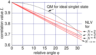
Figure 1: Dependency of the combined correlation parameters $L(\varphi)$ as a function of the separation angle $\varphi$ for the quantum mechanical prediction for a pure singlet state, and bounds for non-local variable models assuming an averaging over various numbers of directions $N$.

The inequality for $N=1$ cannot be violated because $u_{1}=0$ . Already for $N=2$, however, quantum physics violates the inequality: this opens the possibility for our falsification of Leggett’s model without additional assumptions . For $N\rightarrow\infty$, $u_{N}\rightarrow\frac{2}{\pi}$: one recovers inequality (6). The suitable range of difference angles $\varphi$ for probing a violation of the inequalities (9) can be identified from figure 1. The largest violation for an ideal singlet state would occur for $|\sin\frac{\varphi}{2}|=\frac{u_{N}}{4}$, i.e. at $\varphi=14.4^{\circ}$ for $N=2$, increasing with $N$ up to $\varphi=18.3^{\circ}$ for $N\rightarrow\infty$.

Figure 2: Experimental setup. Polarization-entangled photon pairs are generated in Barium-beta-borate (BBO) by parametric down conversion of light from an Ar ion pump laser (PL). After walk-off compensation ($\lambda/2$, CC), down-converted light is collected behind interference filters (IF) into birefringence-compensated (FPC) single mode optical fibers (SMF). Polarization measurements are carried out with a combination of a quarter wave plate ($\lambda/4$) and polarization filters (PF) in front of photon counting detectors D_1,2. The measurement basis for each arm (1,2) is chosen by rotation of the wave plate and polarizing filter by angles $\alpha_{1,2},\beta_{1,2}$ accordingly.

Experiment. We begin with a traditional parametric down conversion source kwiat:95 for polarization-entangled photon pairs with optimized collection geometry in single mode optical fibers kurtsiefer:01 (Fig. 2). Light from a continuous-wave Ar-ion laser at 351 nm is pumping a 2 mm thick barium-beta-borate crystal, cut for type-II parametric down conversion to degenerate wavelengths of 702 nm with a Gaussian spectral distribution of 5 nm (FWHM). We chose a pump power of about 40 mW to ensure both single frequency operation of the pump laser and to avoid saturation effects in the photodetectors. Collection of down-converted light into single mode optical fibers ensures a reasonably high polarization entanglement to begin with. In this configuration, we observed visibilities of polarization correlations of $>98\%$ both in the HV and $\pm 45^{\circ}$ linear basis for polarizing filters located before the fibers. In order to avoid a modulation of the collection efficiency with optical components due to wedge errors in the wave plates, we placed subsequent polarization analyzing elements behind the fiber.

The projective polarization measurements for the different settings of the two observers were carried out using quarter wave plates, rotated by motorized stages by respective angles $\alpha_{1,2}$, and absorptive polarization filters rotated by angles $\beta_{1,2}$ in a similar way with an accuracy of 0.1 degree. This combination allows to project on arbitrary elliptical polarization states. Finally, photodetection was done with passively quenched silicon avalanche diodes, and photon pairs originating from a down conversion process were identified by coincidence detection. The compensator crystals (CC) and fiber birefringence compensation (FPC) were adjusted such that we were able to detect photon pairs in a singlet state.

After birefringence compensation of the optical fibers, we observed the corresponding polarization correlations between both arms with a visibility of $99.5\pm 0.2$% in the HV basis, $99.0\pm 0.2$% in the $\pm 45^{\circ}$ linear basis, and $98.2\pm 0.2$% in the circular polarization basis. Typical count rates were 10100 s^-1 and 8000 s^-1 for single events in both arms, and about 930 s^-1 for coincidences for orthogonal polarizer positions. We measured an accidental coincidence rate using a delayed detector signal of $0.41\pm 0.07\,$s^-1, corresponding to a time window of 5 ns.

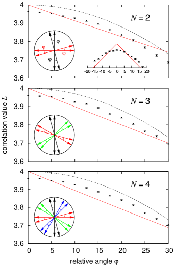
Figure 3: Experimental results for the observed correlation parameters $L_{N}$ (dots), the quantum mechanical prediction for a pure singlet state (curved lines, dashed), and the bounds for the non-local variable models (almost straight lines). In all cases, our experiment exceeds the NLV bounds for appropriate difference angles $\varphi$.

The two orthogonal planes we used in the Poincaré sphere included all the linear polarizations for one, and H/V linear and circular polarizations for the other. That way, we intended to take advantage of the better polarization correlations in the ’natural’ basis HV for the down conversion crystal. Each of the $4N$ correlation coefficients $C(\vec{a},\vec{b})$ in (9,10) was obtained from four settings of the polarization filters via

$$C\big{(}\vec{a},\vec{b}\big{)}=\frac{n_{\vec{a},\vec{b}}+n_{-\vec{a},-\vec{b}}-n_{-\vec{a},\vec{b}}-n_{\vec{a},-\vec{b}}}{n_{\vec{a},\vec{b}}+n_{-\vec{a},-\vec{b}}+n_{-\vec{a},\vec{b}}+n_{\vec{a},-\vec{b}}}$$ (12)

from the four coincident counts $n_{\pm\vec{a},\pm\vec{b}}$ obtained for a fixed integration time of $T=4$ s each. For $N=2,3$ and 4, we carried out the full generic set of 8, 12, and 16 setting groups, respectively, with each $E_{j}^{N}(0)$ containing a HV analyzer setting.

A summary of the values of $L$ corresponding to inequalities for $N=2$, 3 and 4 are shown in Fig. 3, together with the corresponding bounds (9) and the quantum expectation for a pure singlet state (11). The corresponding standard deviations in the results were obtained through usual error propagation assuming Poissonian counting statistics and independent fluctuations on subsequent settings. For $N=2$, we already observe a clear violation of the NLV bound; the largest violation we found was for $N=4$ with about 17 standard deviations above the NLV bound. As expected, the experimental violation increases with growing number of averaging settings $N$. Selected combinations of ($N,\varphi$) violating NLV bounds are summarized in table 1.

$N$	$\varphi$	$L_{\rm NLV}$	$L_{\rm exp}\pm\sigma$	$L_{\rm exp}-L_{\rm NLV}$
2	12.5∘	3.8911	$3.9127\pm 0.0033$	6.45 $\sigma$
2	15∘	3.8695	$3.8970\pm 0.0036$	7.59 $\sigma$
2	17.5∘	3.8479	$3.8638\pm 0.0042$	3.83 $\sigma$
3	12.5∘	3.8743	$3.9140\pm 0.0027$	14.77 $\sigma$
3	15∘	3.8493	$3.8930\pm 0.0030$	14.58 $\sigma$
3	17.5∘	3.8243	$3.8608\pm 0.0034$	10.67 $\sigma$
3	20∘	3.7995	$3.8400\pm 0.0036$	11.15 $\sigma$
4	12.5∘	3.8686	$3.9091\pm 0.0024$	17.01 $\sigma$
4	15∘	3.8424	$3.8870\pm 0.0026$	16.84 $\sigma$
4	17.5∘	3.8164	$3.8656\pm 0.0029$	17.11 $\sigma$

Table 1: Selected values of $L$ violating the NLV bounds $L_{\rm NLV}$ for different averaging numbers $N$.

Our results are well-described assuming residual colored noise in the singlet state preparation cabello:05 . We attribute the small asymmetry of $L_{\rm exp}$ in $\varphi$ (see inset in Fig. 3) to polarizer alignment accuracy.

Overview and Perspectives. After the very general motivation sketched in the introduction, we have focused on Leggett’s model. Let’s now set this model in a broader picture. Non-locality having being demonstrated, the only classical mechanism left to explain quantum correlations is the exchange of a signal. It is therefore natural to assume, as an alternative model to quantum physics, that the source produces independent particles, which later exchange some communication. Sure, this communication should travel faster than light, so the model has to single out the frame in which this signal propagates: it can be either a preferred frame (“quantum ether”), in which case even signaling is not logically contradictory ebe ; or a frame defined by the measuring devices, in which case the model departs from the quantum predictions when the devices are set in relative motion sua97 ; zbi01 . Obviously, there are NLV models that do reproduce exactly the quantum predictions. Explicit examples are Bohmian Mechanics bohm and, for the case of two qubits, the Toner-Bacon model ton03 . Both are deterministic. Now, in Bohmian mechanics, if the first particle to be measured is A, then assumption (2) can be satisfied, but assumption (3) is not. This remark sheds a clearer light on the Leggett model, where both assumptions are enforced: the particle that receives the communication is allowed to take this information into account to produce non-local correlations, but it is also required to produce outcomes that respect the marginals expected for the local parameters alone.

As a conclusion, it must be said that the broad goal sketched in the introduction, namely, to pinpoint the essence of quantum physics, has not been reached yet. However, Leggett’s model and its conclusive experimental falsification reported here have added a new piece of information towards this goal.

Acknowledgements. We are grateful to Anthony J. Leggett, Artur Ekert and Jean-Daniel Bancal for fruitful discussions. C.B. acknowledges the hospitality of the National University of Singapore. This work was partly supported by ASTAR grant SERC-052-101-0043, by the European QAP IP-project and by the Swiss NCCR “Quantum Photonics”.

References

- (1) J.S. Bell, Physics 1, 195 (1964)
- (2) S. Popescu and D. Rohrlich, Found. Phys. 24, 379–385 (1994).
- (3) See e.g. N.J. Cerf, N. Gisin, S. Massar, S. Popescu, Phys. Rev. Lett. 94, 220403 (2005); N. Brunner, N. Gisin, V. Scarani, New J. Phys. 7, 88 (2005); N. Linden, S. Popescu, A.J. Short, A. Winter, quant-ph/0610097; H. Barnum, J. Barrett, M. Leifer, A. Wilce, quant-ph/0611295.
- (4) A.Suarez, V. Scarani, Phys. Lett. A 232, 9 (1997)
- (5) H. Zbinden, J. Brendel, N. Gisin, W. Tittel, Phys. Rev. A 63, 022111 (2001); A. Stefanov, H. Zbinden, N. Gisin, A. Suarez, Phys. Rev. Lett. 88, 120404 (2002)
- (6) A.J. Leggett, Found. Phys. 33, 1469 (2003)
- (7) S. Gröblacher, T. Paterek, R. Kaltenbaek, Č. Brukner, M. Zukowksi, M. Aspelmeyer, A. Zeilinger, Nature 446, 871 (2007)
- (8) Supplementary information of Ref. gro07 .
- (9) S. Parrott, arXiv:0707:3296
- (10) P.G. Kwiat, K. Mattle, H. Weinfurter, A. Zeilinger, A.V. Sergienko, Y. Shih, Phys. Rev. Lett. 75, 4337 (1995)
- (11) C. Kurtsiefer, M. Oberparleiter, H. Weinfurter, Phys. Rev. A 64, 023802 (2001)
- (12) A. Cabello, A. Feito, A. Lamas-Linares, Phys. Rev. A 72, 052112 (2005)
- (13) Ph. Eberhard, A Realistic Model for Quantum Theory with a Locality Property, in: W. Schommers (ed.), Quantum Theory and Pictures of Reality (Springer, Berlin, 1989)
- (14) D. Bohm, B.J. Hiley, The undivided universe (Routledge, New York, 1993)
- (15) B. F. Toner, D. Bacon, Phys. Rev. Lett. 91, 187904 (2003)