Conversion of electron spectrum associated with fission into the antineutrino spectrum

Abstract

The accuracy of the procedure that converts the experimentally determined electron spectrum associated with fission of the nuclear fuels ²³⁵U, ²³⁹Pu, ²⁴¹Pu, and ²³⁸U into the $\bar{\nu}_{e}$ spectrum is examined. By using calculated sets of mutually consistent spectra it is shown that the conversion procedure can result in a small $\sim$1% error provided several conditions are met. Chief among them are the requirements that the average nuclear charge $\langle Z\rangle$ as a function of the $\beta$ decay endpoint energy is independently known and that the $\bar{\nu}_{e}$ spectrum is binned into bins that are several times larger than the width of the slices used to fit the electron spectrum.

I Introduction

Good knowledge of the $\bar{\nu}_{e}$ spectra of nuclear power reactors is an important ingredient of the study of neutrino oscillations with reactors RMP . The next generation of oscillation experiments (e.g. Daya-Bay Daya and Double Chooz DCH ) aim at an unprecendented accuracy in their search for the mixing angle $\theta_{13}$. Even though the multi-detector scheme used in them will greatly reduce the dependence on knowledge of the reactor spectrum, a better understanding of it, and the corresponding error bars, would be clearly beneficial. Nuclear reactor monitoring with neutrinos is another potential application of the reactor $\bar{\nu}_{e}$ detection Cribier . Again, good understanding of the spectrum and its errors is a necessary condition for its success.

The power in nuclear reactors originates in the (time dependent) contribution of fission of four nuclear fuels: ²³⁵U, ²³⁹Pu, ²⁴¹Pu, and ²³⁸U. During a typical fuel cycle the dominant contribution of ²³⁵U at the beginning of the cycle slowly decreases, and the contribution of the reactor produced nuclei ²³⁹Pu and ²⁴¹Pu increases. While ²³⁸U represents $\sim$ 97% of the fresh fuel rods, its fission, caused only by the fast neutrons, contributes only about 10% of the reactor power and changes little during the refueling cycle. In order to determine the reactor $\bar{\nu}_{e}$ spectrum, and its time development, one has to know, therefore, the corresponding $\bar{\nu}_{e}$ spectra associated with the delayed $\beta$ decay of the neutron rich fission fragments of these four fuels.

There are two principal approaches to the determination of the $\bar{\nu}_{e}$ spectra of the individual nuclear fuels. One of them combines knowledge of the fission yields, i.e., the probabilities of populating the individual fission fragments characterized by their mass $A$ and charge $Z$, with the knowledge of their, often complex, $\beta$ decay. The $\bar{\nu}_{e}$ spectrum is then the sum of the contributions of all $\beta$ branches of all fission fragments. The main source of uncertainty of this method is the fact that the $\beta$ decay characteristics of some fission fragments are unknown (or poorly determined), particularly for those with very short lifetimes and hence high $Q$ values. It is then necessary to use various nuclear models in order to characterize the $\beta$ decay of these “unknown” nuclei.

The other approach is based on the experimentally determined electron spectrum associated with fission of the individual fuels which is “converted” into the $\bar{\nu}_{e}$ spectrum. The resulting spectrum uncertainty is then a combination of the experimental uncertainties of the electron spectrum and the uncertainty of the conversion procedure. The accuracy of the conversion procedure is the topic of the present work.

The electron spectra corresponding to the thermal neutron fission of ²³⁵U, ²³⁹Pu and ²⁴¹Pu were measured in a series of experiments using the beta spectrometer BILL at the ILL High Flux Reactor in Grenoble Schreck in 1982-1989. In the quoted papers the electron spectra were converted into the $\bar{\nu}_{e}$ spectra. These spectra, supplanted by the calculated spectrum of ²³⁸U (typically from Ref. Vog ), were used in the analysis of essentially all oscillation experiments performed so far. At short distances from the reactor they agree quite well with the measured $\bar{\nu}_{e}$ signal RMP .

The conversion procedure used in Refs. Schreck is only briefly described there. The corresponding error is estimated to be 3-4% with a weak energy dependence. Since the statistical and normalization errors of the electron spectra usually exceeded the estimated conversion uncertainty, its precise value was less important so far. Here, I wish to return to this issue, two decades later, in order to determine the uncertainty in the conversion procedure more firmly, and study its possible optimization.

II Conversion for one nucleus

Throughout this work it is assumed that all relevant $\beta$ decays have the allowed shape. The possible effects associated with the unique first forbidden decays (and higher order forbidden decays) are neglected. Thus, the electron spectrum is assumed to be of the shape

$$N(E_{e})=k(E_{0},Z)E_{e}p_{e}(E_{0}-E_{e})^{2}F(Z+1,E_{e})~{},$$ (1)

where $k(E_{0},Z)$ is the normalization constant, $E_{e}$ and $p_{e}$ are the full electron energy and momentum, and $F(Z+1,E_{e})$ describes the Coulomb effect on the outgoing electron. The $\bar{\nu}_{e}$ spectrum as a function of the antineutrino energy $E_{\nu}$ is obtained from eq.(1) by substituting $E_{\nu}=E_{0}-E_{e}$ in the above formula.

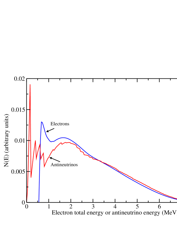
Figure 1: (Color online) Example of complex electron and corresponding $\bar{\nu}_{e}$ spectra. This example is for a hypothetical $\beta$ decay of a $Z=45$ nucleus with 40 branches. The endpoints are randomly distributed, with average spacing of 200 keV, and the largest kinetic energy of the electrons is 8 MeV. The branching ratios are also randomized.

For a single branch decay, therefore, the conversion procedure is a trivial one. Note the basic differences between the electron and $\bar{\nu}_{e}$ spectrum in that case. There is a finite probability of emission of an electron with vanishing momentum. Thus, the electron spectrum begins at a finite value at $E_{e}=m_{e}~{}(p_{e}=0)$, while the $\bar{\nu}_{e}$ spectrum vanishes for $E_{\nu}=0$. On the other hand, near the endpoint the electron spectrum vanishes as $E_{e}\rightarrow E_{0}$, while the $\bar{\nu}_{e}$ spectrum approaches a finite value as $E_{\nu}\rightarrow E_{0}-m_{e}$. Moreover, since electrons are attracted to the positively charged nucleus the electron spectrum reaches its maximum at lower energies than the $\bar{\nu}_{e}$ spectrum.

An illustrative example of a complex spectrum is shown in Figure 1. Note that the full electron energy is used on the x-axis; hence the electron spectrum begins at $m_{e}$. Due to the differences listed above the smooth electron spectrum is associated with a jagged $\bar{\nu}_{e}$ spectrum. That is most noticeable at low energies, while at higher energies the two spectra are quite similar. (The very upper edge is not shown. Naturally the electron spectrum extends $m_{e}$ further than the $\bar{\nu}_{e}$ spectrum.)

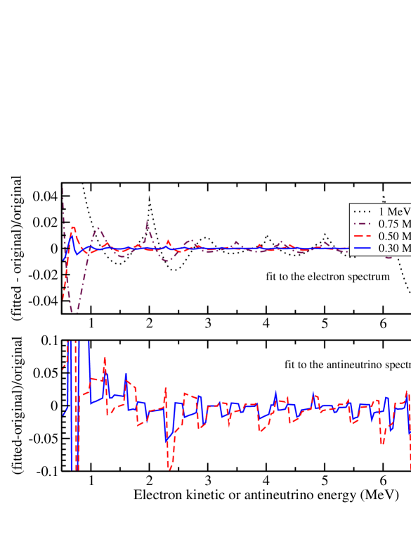
Figure 2: (Color online) The fit to the complex spectra in Figure 1. In the upper panel the smooth electron spectrum is fitted. The size of the slices and the corresponding notation is indicated. The plotted quantity is the normalized deviation of the fitted spectrum from the original one. In the lower panel the endpoints and intensities of the fitted branches from the electron spectrum are used to reconstruct the $\bar{\nu}_{e}$ spectrum. Its normalized deviation from the true original $\bar{\nu}_{e}$ spectrum is plotted for two slice intervals (300 keV - full line and 500 keV - dashed line). Note the change of scale between the panels.

Let assume that the electron spectrum in Fig. 1 has been experimentally determined, but the endpoints and intensities of the individual branches remain unknown. How can one convert the electron spectrum into the $\bar{\nu}_{e}$ one? The procedure used in Refs. Schreck is sensible and practical. The electron spectrum is divided into a number $n$ of slices. In Schreck these slices are all of equal width, and that choice again is simplest and economical, since it minimizes the number of free parameters. Then, starting with the highest energy slice, one assumes the allowed shape, Eq.(1), and fits for the corresponding endpoint and intensity. Once these parameters were determined, the resulting branch spectrum is extended down to $E_{e}=m_{e}$ and subtracted from the full spectrum. The procedure is then repeated for the next slice, etc., until all $n$ slices (or assumed branches) are characterized by their endpoints and intensities. The free parameter $n$, the number of assumed branches, is then optimized so that the true original experimental electron spectrum, and the fitted one, are as close to each other as possible.

Since the electron spectrum is always a smooth function of energy, the procedure works well, as demonstrated in the upper panel of Fig. 2. For slices of 0.3 or 0.5 MeV width the maximum deviation is less than 1%, except for the lowest and highest electron energies. (Since the spectrum is assumed to be measured in a finite number of points, every 50 keV in this example, the number of slices $n$ is constrained also from above.) Having approximated the complex $\beta$ decay scheme by $n$ fictitious branches characterized by their endpoints and branching ratios, one can construct the corresponding $\bar{\nu}_{e}$ spectrum. Comparing it to the true original spectrum, one can see that the fit is less perfect (see the lower panel in Fig. 2). That is not surprising. The steps associated with true endpoints cannot be faithfully reproduced by the fit, hence the jagged form in Fig. 2. For practical application this is less important; if the $\bar{\nu}_{e}$ spectrum is binned in bins wider than the slices of the fit, the up and down features in Fig. 2 would be smoothed out.

III Spectrum of fission fragments

The fission fragments are broadly distributed in nuclear masses and charges. For example, the calculations used in Ref. Vog were based on 1153 different fission fragments ranging from $Z,A$ = 23,66 to 72,172. Most of them are radioactive, and many have complex $\beta$ decay schemes. The resulting electron and $\bar{\nu}_{e}$ spectra are therefore superpositions of many thousands of $\beta$ decay transitions.

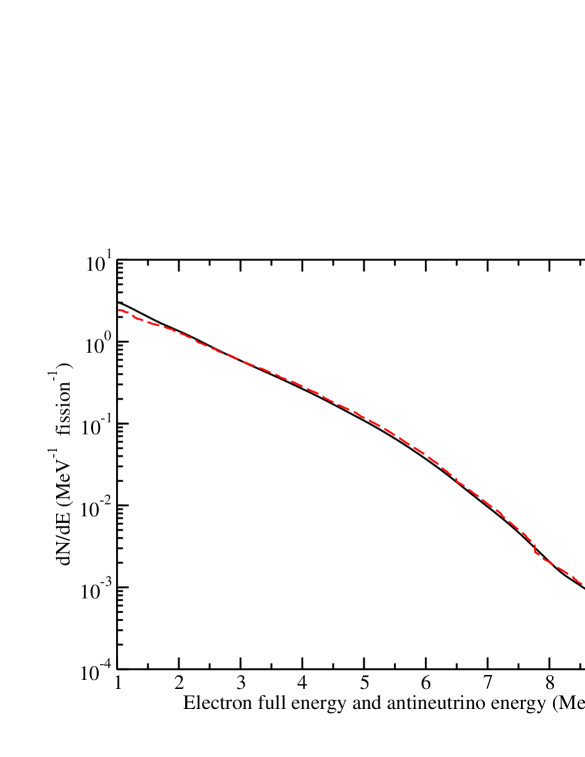
Figure 3: (Color online) Calculated spectra of electrons and $\bar{\nu}_{e}$ corresponding to the thermal neutron fission of ²³⁵U at equilibrium.

An example of the calculated electron and $\bar{\nu}_{e}$ spectra is shown in Fig. 3. They correspond to the thermal neutron fission of ²³⁵U using the data files in Ref. Vog . Clearly, within the rather coarse scale of the figure, the two spectra are essentially identical; thus the conversion procedure should work well. Both spectra, calculated with a fine step of 10 keV, appear to be smooth. In the case of $\bar{\nu}_{e}$ this is so because so many $\beta$ decays contribute that the step at the endpoint of each of them is not noticeable.

The equilibrium spectrum in Fig. 3 is calculated using

$$\frac{dN}{dE_{e}}=\Sigma_{A,Z}Y(Z,A)\Sigma_{i}b_{i}E_{e}p_{e}(E_{0}^{i}-E_{e})^{2}F(Z+1,E_{e})~{},$$ (2)

where $Y(Z,A)$ are the cummulative fission yields, and $b_{i}$ are the $\beta$ decay branching ratios of the $i$th branch of the fragment $Z,A$ with endpoints $E_{0}^{i}$. The $\bar{\nu}_{e}$ spectrum is obtained from the same formula by the substitution $E_{\nu}=E_{0}^{i}-E_{e}$ for every branch.

As stated above, the allowed shape is assumed for all $\beta$ branches. This assumption should not affect the conclusions of this work, which is based on the consistent comparison of the converted $\bar{\nu}_{e}$ spectrum with the calculated spectrum using Eq. (2). On the other hand, the actual spectrum associated with fission will clearly contain a number of forbidden $\beta$ transitions. Among them the nonunique first forbidden ones have usually allowed shapes anyway, and the higher order forbidden decays could be safely neglected. It is difficult to estimate the error associated with the neglect of the known shape factor of the unique first forbidded $\beta$ decays, but it is not expected to be significant, since the converted $\bar{\nu}_{e}$ spectra agree well with measurements at close distances from the reactor RMP .

Now, let us use the conversion procedure described above and convert the electron spectrum, assumed to be known accurately, into the $\bar{\nu}_{e}$ spectrum. When the smooth electron spectrum is divided into $n$ slices of sufficiently narrow width, each slice can be well reproduced as a piece of the allowed spectrum, Eq.(1). There is only one parameter to fit for each slice, the endpoint $E_{0}$, while the normalization is determined automatically. The dependence on the nuclear charge $Z$ is rather weak, a good fit is obtained with a constant $Z$.

Figure 4: (Color online) Deviations of the fit for the electron (dashed line; deviations very small and not visible in the plot) and $\bar{\nu}_{e}$ spectra, calculated with a constant $Z$ = 47. The fit with 100 keV slices is the jagged line; interpolating the antineutrino spectrum over 250 keV wide bins the smoother line results. The spectra are for the thermal neutron fission of ²³⁵U at equilibrium as in Fig. 3.

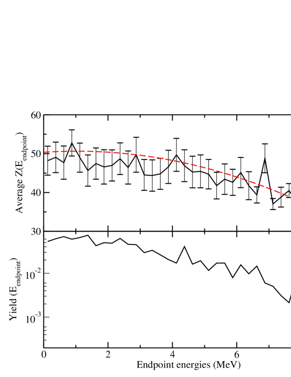
Figure 5: (Color online) Average nuclear charge $\langle Z\rangle$ as a function of the $\beta$ decay endpoint energy (in 0.25 MeV steps) for the ²³⁵U fission by thermal neutrons. (For the definition of $\langle Z\rangle$ and its variance see text). The quadratic polynomial $Z(E_{0})$ that gave the best fit to the $\bar{\nu}_{e}$ spectrum is shown by the dashed line. The lower panel shows, in log scale, the fission yield as a function of $E_{endpoint}$.

Having the set of $n$ endpoints and branching ratios, one can again reconstruct the $\bar{\nu}_{e}$ spectrum and compare it with the $\bar{\nu}_{e}$ spectrum derived from eq. (1). There one encounters two problems. First, instead of many thousands of branches, there is now a much smaller number $n$ of branches. Hence, the steps at the endpoint of each branch become more pronounced in comparison with the true $\bar{\nu}_{e}$ spectrum. Second, the choice of the nuclear charge $Z$ becomes important, unlike in the fit of the electron spectrum. These features are illustrated in Fig.4. There, the fit was performed with a constant Z = 92/2+1 = 47, with slices 100 keV wide which were also rebinned to 250 keV wide bins. The electron spectrum, with or without binning, is reproduced perfectly, with deviations of $\sim 10^{-4}$. On the other hand, the $\bar{\nu}_{e}$ spectrum is not fitted very well. Without binning one can clearly see the steps caused by the fit. They disappear with binning, but the overall fit, particularly at higher energies, is not very good. That is caused by the choice of the fixed nuclear charge $Z$.

It turns out that different $Z$ values contribute to different parts of the spectrum. This is shown in Fig. 5. There, for each bin with the endpoint $E_{0}$ the quantity $\langle Z\rangle$ is calculated as

$$\langle Z\rangle(E_{0})=\frac{\Sigma_{A,Z}Y(Z,A)\Sigma_{i}b_{i}(E_{0}^{i})Z}{\Sigma_{A,Z}Y(Z,A)\Sigma_{i}b_{i}(E_{0}^{i})}~{}~{},~{}~{}\Delta<Z>=(\langle Z^{2}\rangle-\langle Z\rangle^{2})^{1/2}~{}.$$ (3)

The error bars in Fig. 5 are the dispersion $\Delta<Z>$ of the $Z$ values within each bin. One can see clearly the slope of the $\langle Z\rangle(E_{0})$ function; the $\langle Z\rangle$ values are decreasing with increasing $E_{0}$. At the same time, in the lower panel of Fig. 5, one can see that the total fission yield decreases very rapidly with increasing $E_{0}$.

The smooth dashed line in the upper panel of Fig. 5 shows the average nuclear charge $Z$ giving fit to the $\bar{\nu}_{e}$ spectrum that agrees with the original spectrum within 1% in the relevant interval of energies. It is represented by a quadratic polynomial in $E_{0}$ as in some of the Refs. Schreck . The dashed line is above the corresponding $<Z>$ due to the fact that in the eq.(1) $Z+1$ should be used. The quadratic polynomial fits of the form $Z=a+b\times E_{0}+c\times E_{0}^{2}$ were used for all four nuclear fuels, resulting in deviation that does not exceed $\sim$1% as shown in Fig. 6. The corresponding parameters $a,b,c$ are listed in Table I. The procedures (width of the slices and interpolating bins) used in the fits shown in Fig. 6 appear to be close to the optimum required for the precision conversion procedure.

The calculated electron and $\bar{\nu}_{e}$ spectra used for testing the accuracy of the conversion procedure were mutually consistent, but did not contain the small but nonnegligible QED and weak magnetism corrections. In conversion using the experimentally measured electron spectra these corrections should be included. The corresponding formulae can be found e.g. in Refs. Vogel84 ; Fayans85 ; Kurylov03 .

Table 1: Parameters of the polynomial fit $\langle Z\rangle=a+b\times E_{0}+c\times E_{0}^{2}$ of the average nuclear charge as a function of the endpoint energy for the indicated isotopes

nucleus	$a$	$b$	$c$
235U	50.0	0.825	-0.269
239Pu	50.0	0.825	-0.250
241Pu	50.0	0.825	-0.220
238U	50.5	0.825	-0.220

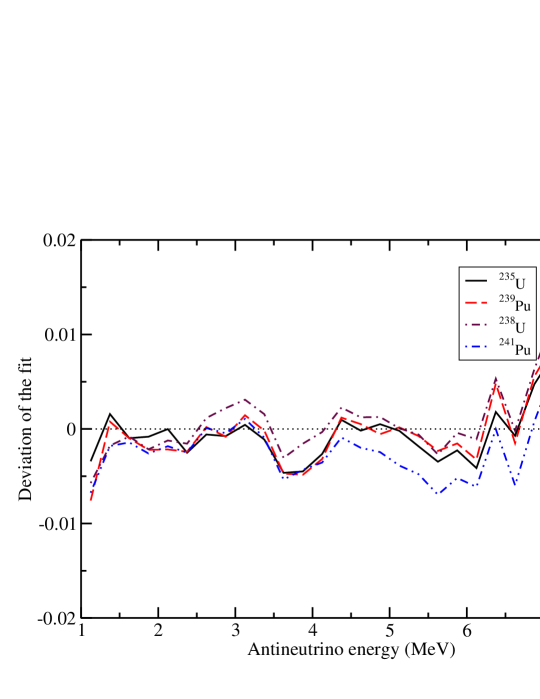
Figure 6: (Color online) Deviations of the $\bar{\nu}_{e}$ fits using the quadratic polynomial expression for nuclear charge dependence on the endpoint, $Z(E_{0})$ (see Table I), for the indicated nuclear fuels. Input spectra with 10 keV intervals were fitted in 100 keV wide slices which were then interpolated into 250 keV wide bins.

IV Conclusion

Using the mutually consistent sets of the realistic electron and $\bar{\nu}_{e}$ spectra corresponding to the fission of the nuclear fuels ²³⁵U, ²³⁹Pu, ²⁴¹Pu, and ²³⁸U I have shown that the electron spectrum can be converted into the $\bar{\nu}_{e}$ spectrum with an error that does not exceed $\sim$1% in the energy interval 1 - 8 MeV. However, such accurate conversion can be obtained only if several conditions are met:

• The slices into which the electron spectrum is divided are sufficiently fine.

• The converted $\bar{\nu}_{e}$ spectrum is smoothed out by binning in bins that are several times larger than the width of the original slices.

• The optimum average nuclear charge $\langle Z\rangle$ is independently known as a function of the endpoint energy $E_{0}$.

Not all these criteria were fulfilled in Refs. Schreck , hence the larger uncertainties associated with the conversion procedure assigned there cannot be safely reduced. The electron spectra in Schreck were published in 250 keV wide bins. The number of bins and the number of slices for the conversion procedure were the same (or nearly so). The smooth electron spectra were expressed in the Fermi-Kurie representation which made the corresponding fits possible. And the $\bar{\nu}_{e}$ spectra were not rebinned, thus the steps at the edges of slices were not smoothed out. However, as already pointed out above, the statistical and systematic errors of the measured electron spectra mostly exceeded the errors of the conversion procedure, so even if it would be somehow possible to minimize the uncertainty of the conversion procedure, it would affect the spectra of Refs. Schreck only minimally. They remain the best existing source of the fission associated $\bar{\nu}_{e}$ spectra.

The main purpose of the present work is an examination of the conversion procedure per se. While there are no immediate plans to repeat and/or improve the results of the experiments in Refs. Schreck , there exist measurements of the $\beta$ spectra of many individual neutron rich fission fragments (see, e.g. Allek ; Tengb ). These, in turn, can be converted into the $\bar{\nu}_{e}$ spectra using the procedure described here, and combined with the fission yields to obtain the full $\bar{\nu}_{e}$ spectrum. Similar measurements of individual short lived (and high $Q$ value) fission fragments can be performed with the modern isotope separation facilities. Thus, significant improvements of the determination of the reactor $\bar{\nu}_{e}$ spectra is possible. The present work is part of that effort.

V Acknowledgment

The work reported here was supported in part by the US Department of Energy contract DE-FG02-05ER41361. The author deeply appreciates the hospitality of Prof. Cristina Volpe and the Institut de Physique Nucléaire, Orsay, where part of this research was performed.

References

- (1) C. Bemporad, G. Gratta and P. Vogel, Rev. Mod. Phys. 74, 297 (2002).
- (2) Daya-Bay collaboration, arXiv: hep-ex/0701029.
- (3) F. Ardellier et al., arXiv:hep-ex/0606025.
- (4) M. Cribier, arXiv:0704.0548; arXiv:0704:0891.
- (5) F. von Feilitzsch, A.A.Hahn and K. Schreckenbach, Phys. Lett. 118B, 162 (1982); K. Schreckenbach, G. Colvin, W. Gelletly and F. von Feilitzsch, Phys. Lett. 160B, 325 (1985); A. A. Hahn et al. Phys. Lett. 218B, 365 (1989).
- (6) B. R. Davis, P. Vogel, F. M. Mann and R. E. Schenter, Phys. Rev C19, 2259 (1979); P. Vogel, G. K. Schenter, F. M. Mann and R. E. Schenter, Phys. Rev. C24, 1543 (1981).
- (7) P. Vogel, Phys. Rev. D29, 1918 (1984).
- (8) S. A. Fayans, Sov. J. Nucl. Phys. 42, 590 (1985).
- (9) A. Kurylov, M. J. Ramsey-Musolf and P. Vogel, Phys. Rev. C67, 035502 (2003).
- (10) K. Aleklett, G. Nyman, and G. Rudstam, Nucl. Phys. A246, 425 (1977).
- (11) O. Tegblad et al., Nucl. Phys. A503, 136 (1989).