We present a novel approach to look for the existence of maximum entanglement in a system of two identical quantum dots coupled by the Fö rster process and interacting with a classical laser field. Our approach is not only able to explain the existing treatments, but also provides further detailed insights into the coupled dynamics of quantum dots systems. The result demonstrates that there are two ways for generating maximum entangled states, one associated with far off-resonance interaction, and the other associated with the weak field limit. Moreover, it is shown that exciton decoherence results in the decay of entanglement.

1 Introduction

Quantum dots are semiconductor structures containing a small number of electrons within a region of space with typical sizes in the sub-micrometer range [1]. Coupling of two quantum dots leads to double quantum dots, which in analogy with atomic and molecular physics, is described as two-level systems with controllable level-spacing and one additional transport electron [2]. This rather suggests the analogy with a simple model for an atom, in particular if it comes to interaction with external fields such as photons or phonons. Many properties of such systems can be investigated by transport, if the dots are fabricated between contacts acting as source and drain for electrons which can enter or leave the dot. The possibility of using pairs of quantum dots coupled by the dipole-dipole interaction as effective three- or four-level systems whose transmission for an optical beam at some frequency may be switched on or off using a second optical beam has been explored [3]. In contrast to real atoms, quantum dots are open systems with respect to the number of electrons which can easily be tuned with external parameters such as gate voltages or magnetic fields [4, 5].

The experimental realization of optically induced entanglement of excitons in a single quantum dot [6] and theoretical study on coupled quantum dots [7] have been reported recently. In those investigations a classical laser field is applied to create the electron-hole pair in the dot(s). Several groups have performed transport experiments with double quantum dots, with lateral structures offering experimental advantages over vertical dots with respect to their tunability of parameters [8]. However, in contrast to atomic systems carrier lifetimes in the solid state are much shorter because of the continuous density-of-states of charge excitations and stronger environment coupling [9, 10].

Recently a major advancement in the field has come from different types of local optical experiments, that allow the investigation of individual quantum dots thus avoiding inhomogeneous broadening and simple coherent-carrier control in single dots [11]. Some quantum information processing schemes have been proposed exploiting exchange and/or direct Coulomb interactions between spatially separated excitonic qubits in coupled quantum dots systems [7, 12, 13, 14]. Using far-field light excitation to globally address two and three quantum dots in a spatially symmetric arrangement and preparations of both Bell and Greenberger-Horne-Zeilinger entangled states of excitons have been discussed [12, 13]. Also, an alternative scheme for a three-qubit entangled state generation by nonlinear optical state truncation has been introduced [15].

Based on adiabatic elimination treatment [2], the creation of two-particle entangled states in a system of coupled quantum dots have been discussed. The authors of this study avoided dealing with the exact solution of the problem and employed the adiabatic elimination as an approximate treatment. However, one should be aware that its predictions for any coupled system need to be checked against the exact solution of the complete coupled equations. In order to avoid such limitations, one must begin by ignoring any approximation and try to find an analytical solution of the coupled equations that govern the system. At this point, there is no generally established approach that can provide a complete description of the dynamics for the system. It is the purpose of this paper to present such an approach with illustrative applications. The basic idea relies on the discretization of the coupled system, which is thus replaced in the formulation by only linear solvable equation. Related treatments based on either adiabatic elimination [2, 16, 17], discussing entangled state generation conditions, or the coupled equations without the detuning dependence, have been presented in the literature [5].

What we study and present below is essentially a most general case of the complete equations of the two-quantum dots system. Most interestingly, it is shown that features of the degree of entanglement are influenced significantly by different values of the involved parameters and exciton decoherence. With this approach we could create a two-particle entangled state between the vacuum and bi-exciton states or single-exciton entangled state, without using the approximation method adopted in previous studies.

The outline of this paper is arranged as follows: in section 2, we give notation and definitions of the model. To reach our goal, an analytical approach for obtaining exact-time dependent expressions for the probability amplitudes is developed in section 2.1 and exciton decoherence is discussed in section 2.2. Having obtained the solution, in section 3, we analyze the time evolution of the populations of the quantum levels for various values of the system parameters. In section 4, we study the evolution of the degree of entanglement, measured by the negativity measure for the partial transpose density matrix. Finally, our conclusion is presented in section 5.

2 Model

The model under consideration consists of two identical quantum dots coupled by the Förster process [18, 19, 20, 21]. This process originates from the Coulomb interaction whereby an exciton can hop between the two dots [18]. The quantum dots contain no net charge and interact with a high frequency laser pulse. This in effect means that the present model has three processes: (i) the coupling of the carrier system with a classical laser field, (ii) the interdot Förster interaction and (iii) the single-exciton, keeping in mind the fact that all constant energy terms may be ignored. The total Hamiltonian for the quantum-dot system is given by [22],

$$\hat{H} = \frac{\hbar}{2}\sum\limits_{j=1,2}\left(\Omega\exp\left[-i\omega t+i\phi\right]\widehat{e}_{j}^{\dagger}\widehat{\psi}_{j}^{\dagger}+\Omega^{\ast}\exp\left[i\omega t-i\phi\right]\widehat{\psi}_{j}\widehat{e}_{j}\right)$$ (1)

$$-\frac{1}{2}\sum\limits_{j=1}^{2}\left\{\sum\limits_{k=1}^{2}\hbar\eta\left(\widehat{e}_{j}^{\dagger}\widehat{\psi}_{k}\widehat{e}_{k}\widehat{\psi}_{j}^{\dagger}+\widehat{\psi}_{j}\widehat{e}_{k}^{\dagger}\widehat{\psi}_{k}^{\dagger}\widehat{e}_{j}\right)-\varepsilon\left(\widehat{e}_{j}^{\dagger}\widehat{e}_{j}-\widehat{\psi}_{j}\widehat{\psi}_{j}^{\dagger}\right)\right\},$$

where $\Omega$ represents the laser-quantum dot coupling and $\hbar\Omega=\mu E$, where $\mu$ is the coupling strength and $E$ is the laser field amplitude. The parameters $\omega$ and $\phi$ describe the angular frequency and phase of the laser field, respectively. The operator $\widehat{e}_{j}(\widehat{\psi}_{j})$ is the electron (hole) annihilation operator and $\widehat{e}_{j}^{\dagger}(\widehat{\psi}_{j}^{\dagger})$ is the electron (hole) creation operator in the $j^{\underline{th}}$ quantum dot. We denote by $\varepsilon$ the band gap energy of the quantum dot and $\eta$ the inter-dot process hopping rate.

For a coupled two-quantum-dot system, it is useful to write the Hamiltonian of equation (1) in the basis $|0\rangle=|0,0\rangle,$ $|1\rangle=\left(|1,0\rangle+|0,1\rangle\right)/\sqrt{2},$ and $|2\rangle=|1,1\rangle$ which describe the vacuum state, the single exciton state, and the biexciton state, respectively. In this system the antisymmetric state $|a\rangle=\left(|1,0\rangle-|0,1\rangle\right)/\sqrt{2}$ is completely decoupled from the remaining states. Then the simple three-state representation of the two-quantum-dot system can be employed with $|0\rangle,$ $|1\rangle$ and $|2\rangle.$ Since the density matrix of the system is diagonal and the symmetric state $|1\rangle$ is a maximally entangled state, an entanglement can be produced in this model by a suitable population of the state $|1\rangle$.

Applying the rotating wave approximation and a unitary transformation, the resulting Hamiltonian may be written as

$$H=2\hbar\Delta\widehat{A}_{22}+\hbar(\Delta-\eta)\widehat{A}_{11}+\frac{\hbar}{\sqrt{2}}\left[\frac{{}}{{}}\Omega e^{i\phi}\left(\widehat{A}_{01}+\widehat{A}_{12}\right)+H.c.\right],$$ (2)

where $\widehat{A}_{ij}=|i\rangle\langle j|,$ related to the above states $|0\rangle,$ $|1\rangle$ and $|2\rangle.$ We denote by $\Delta$ the detuning of the laser frequency from exact resonance ($\hbar\Delta=\varepsilon-\hbar\omega)$.

It is worth mentioning here that, one can take advantage of the Förster interaction between two quantum dots and apply a finite rectangular pulse and sub-picosecond duration to generate a Bell state such as $\alpha|00\rangle+\beta|11\rangle$ where $|11\rangle$ denotes the simultaneous presence of two excitons in a double dot structure. Also, formations of an entangled state between the vacuum and the exciton (or the biexciton) state have been discussed [23, 24].

2.1 An analytic solution

We devote the present section to find an explicit expression for the wave function in Schrödinger picture. We use an analytic approach that seeks to reduce the coupled equations system (probability amplitudes) to a solvable linear equation in order to study in detail the types of interaction that exist between them. To reach our goal we assume that the wave function of the complete system may be expanded in terms of the well known eigenstates $\left|i\right\rangle$, $(i=0,1,2)$, namely

$$\left|\Psi(t)\right\rangle=B_{0}(t)\left|0\right\rangle+B_{1}(t)\left|1\right\rangle+B_{2}(t)\left|2\right\rangle.$$ (3)

The time dependence of the amplitudes in equation (3) is governed by the Schrödinger equation with the Hamiltonian given by equation (2), therefore we obtain

$$i\frac{\partial B_{j}(t)}{\partial t}=\sum\limits_{k=0}^{2}\xi_{jk}B_{k}(t),$$ (4)

where $\xi_{jk}=\left\langle j\right|\hat{H}\left|k\right\rangle.$ In this case and using equations (2) and (3), we obtain $\xi_{01}=\left(\xi_{10}\right)^{\ast}$ $=\xi_{12}=\left(\xi_{21}\right)^{\ast}$ $=\Omega^{\prime}e^{-i\phi},$ $\xi_{11}=\Delta-\eta,$ $\xi_{22}=2\Delta,$ $\Omega^{\prime}=\Omega/\sqrt{2}$  otherwise $\xi_{ij}=0.$

In order to solve equation (4), we introduce the following function [25]

$$G(t)=B_{0}(t)+xB_{1}(t)+yB_{2}(t),$$ (5)

which leads to the equation

$$i\frac{dG(t)}{dt}=\beta\left(B_{0}(t)+\frac{\gamma_{1}}{\beta}B_{1}(t)+\frac{\gamma_{2}}{\beta}B_{2}(t)\right),$$ (6)

where $\beta=x\xi_{10},\gamma_{1}=\xi_{12}+x\xi_{11}+y\xi_{21}$ and${\ \ }\gamma_{2}=x\xi_{12}+y\xi_{22}.$ Now let us seek a solution of $G(t)$ such that $\dot{G}(t)=-izG(t)$. This holds if and only if $z=\beta,x=\gamma_{1}/\beta$ and $\ y=\gamma_{2}/\beta.$

After some minor algebra this leads to a qubic equation which contains $3$ eigenvalues (to determine the $z_{i}$) corresponding to the same number of the eigenfunctions $G_{j}(t)=G_{j}(0)\exp(-iz_{j}t).$ Using equation (5), one can write

$$G_{j}(t)=\sum\limits_{l=1}^{3}O_{jl}\overline{B}_{l}(t),$$ (7)

where $O_{jl}$ is a $3\times 3$ matrix whose elements are $O_{j1}=1,O_{j2}=x_{j}$ and $O_{j3}=y_{j}$ and $\overline{B}_{l}=B_{l+1}.$

Now, we can express the unperturbed state amplitude $\overline{B}_{j}(t)$ in terms of the dressed state amplitudes $G_{j}(t)$ in this form $\overline{B}_{i}(t)=\sum\limits_{j=1}^{3}\left(O^{-1}\right)_{ij}G_{j}(0)\exp(-iz_{j}t).$  Using the above equations, we have

$$\overline{B}_{j}(t)=\lambda_{j1}\exp\left(-iz_{1}t\right)+\lambda_{j2}\exp\left(-iz_{2}t\right)+\lambda_{j3}\exp\left(-iz_{3}t\right),$$ (8)

where

$$z_{j} = -\frac{\xi_{10}}{3}\left[\alpha_{1}+2\left(\alpha_{1}^{2}-3\alpha_{2}\right)^{\frac{1}{2}}\cos\left(\frac{1}{3}\arccos\left(\frac{9\alpha_{1}\alpha_{2}-2\alpha_{1}^{3}-27\alpha_{3}}{2(\alpha_{1}^{2}-3\alpha_{2})^{3/2}}\right)+[j-1]/3\right)\right],$$

$$\alpha_{1} = -\frac{\xi_{11}+\xi_{22}}{\xi_{01}^{\ast}},{\ \ \ \ }\alpha_{2}=-\frac{\xi_{11}\xi_{22}+2|\xi_{01}|^{2}}{\left(\xi_{01}^{\ast}\right)^{2}},{\ \ \ }\alpha_{3}=-\frac{\xi_{22}}{\xi_{01}^{\ast}}.$$

The parameter $\lambda_{ij}=\left(O^{-1}\right)_{ij}G_{j}(0)$ where $\left(O^{-1}\right)_{ij}$ is the ij element of the matrix $O^{-1}$ which is the inverse of the matrix $O$. We have thus completely determined an analytic solution of the coupled quantum dots system in presence of the detuning parameter and phase.

2.2 Quantum decoherence

The original meaning of decoherence was specifically designated to describe the loss of coherence in the off-diagonal elements of the density operator in the energy eigenbasis [26]. Amongst the most crucial requirements for the implementation of quantum logic devices is a high degree of quantum coherence. Coherence is lost when a qubit interacts with other quantum degrees of freedom in its environment and becomes entangled with them. Exciton decoherence in semiconductor quantum dots is affected by many environmental effects, however it is dominated by acoustic phonon scattering at low temperatures [27]. The decoherence effects due to the exciton–acoustic-phonon coupling on the generation of an exciton maximally entangled state in quantum dots were studied in [28]. This process is governed by the Hamiltonian [29]

$$\widehat{H}_{T}=\widehat{H}+\sum_{k}\omega_{k}a_{k}^{{\dagger}}a_{k}+\sum_{k}g_{k}J_{z}\left(a_{k}^{{\dagger}}+a_{k}\right),$$ (9)

where $\widehat{H}$ is given by equation (1) and $a_{k}^{{\dagger}}(a_{k})$ stands for the creation (annihilation) operator of the acoustic phonon with wave vector $k$ and $g_{k}$ the coupling between the dots and the field. By the general procedure, we can deduce a master equation for the density operator $\rho(t)$ of the total system in the following form

$$\frac{\partial}{\partial t}\rho(t)=J\rho(t)+\pounds_{1}\rho(t),$$ (10)

with

$$\pounds_{1}\rho(t)=-i\Gamma[J_{z},[J_{z},\rho(t)]],$$

where the superoperator $J$ is defined as $J\rho(t)=-i[\widehat{H},\rho(t)]$ and $\Gamma$ is the decoherence rate [5]. However its dependence on the mode distribution of phonons as well as a cutoff frequency is given by [30],

$$\Gamma=\int d\omega^{\prime}\omega^{\prime n}\exp\left(\frac{-\omega^{\prime}}{\omega_{c}}\right)(1+2N(\omega^{\prime},T)),$$ (11)

with $n$ depending on the dimensionality of the phonon field, $\omega_{c}$ is a cut-off frequency and $N(\omega^{\prime},T)$ is the phonon occupation factor. Here, we consider pure decoherence effects that do not involve energy relaxation of excitons. The solution of equation (10) can be formally written as

$$\rho(t)=\exp[t\left(J+\pounds_{1}\right)]\rho(0).$$ (12)

Here $\rho(0)$ is the initial state of the system. The decoherence parameter $\Gamma$ is temperature dependent and it amounts for $20-60$ $\mu eV$ for typical semiconductor quantum dots in a temperature range from $10$ $K$ to $30$ $K$ [27, 30]. The results of this analysis are more closely related to experimental situations, which are usually strongly affected by decoherence and relaxation. However, because time scales are very long the relaxation processes are not considered here.

3 Occupation probabilities

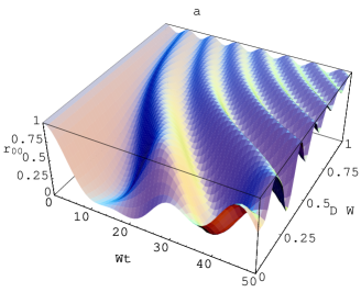
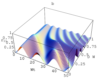
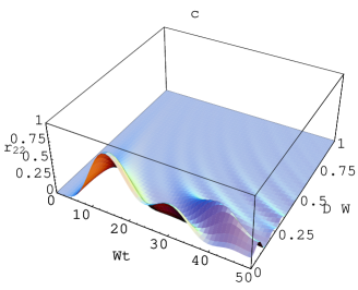
Figure 1: The probability amplitudes as functions of $\Omega t$ and $\Delta/\Omega$. The parameters used in these figures are $\phi=0,\eta/\Omega=0.1$ and $\Gamma=0$.

By making use of the theoretical treatment in the previous section, one can investigate the statistical properties of the system. Using the final state $\left|\Psi(t)\right\rangle$ or $\rho(t)$ all relevant quantities can be computed. In this section, our motivation is to investigate the occupation probabilities associated with two identical quantum dots coupled by the Förster process and interacting with a classical laser field. The expressions $\rho_{ii}(t)=|B_{i}(t)|^{2},$ ($i=0,1,2$) represent the probabilities that at time $t,$ the coupled quantum dots is in the state $|i\rangle$.

In figure 1, we plot the probability amplitudes as functions of the dimensionless parameters $\Omega t$ and $\Delta/\Omega$. The parameters used in these figures are $\phi=0,\eta/\Omega=0.1$ and $\Gamma=0$. It implies that the complete Rabi oscillations between the localized states occur. Once the detuning parameter is taken into account, the populations of biexciton state is decreased (see figure 1c). On further increase of the detuning parameter $\Delta$ one finds that the occupation probability of this level tends to zero, while the oscillations of the other levels show fast oscillations with small amplitudes (see figures 1). From this point of view, the transition can be considered as existing only between two states $|0>$ and $|1>$for larger detuning, which means that the biexciton state is decoupled.

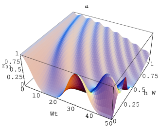
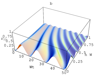
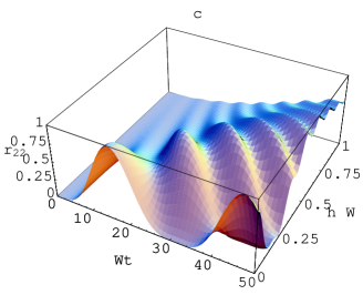
Figure 2: The probability amplitudes as functions of $\Omega t$ and $\eta/\Omega$. Calculations assume that $\phi=0,\Delta/\Omega=0,$ and $\Gamma=0$.

One, possibly not very surprising, principal observation is that the numerical calculations corresponding to the same parameters, which have been considered in [2], gives nearly the same behavior, but with different scaled time. The important consequence of this observation is that using smaller values of the laser-quantum dot coupling, the creation of a two-particle entangled state between the vacuum and the bi-exciton states or a two-particle entangled state between vacuum and single-exciton states, depends essentially on controlling the detuning parameter.

Apart from helping us to know different conditions for creating maximum entangled states, using our exact solution, that would otherwise be very hard to figure out, some of our testing results are of interest. A particularly non-intuitive one is the following: previously, we used to think that increasing the detuning parameter always decreases the populations of the single-exciton state or bi-exciton state, depending on its relation with the laser-dot coupling parameter. But, in figure 2 even with fixing the detuning parameter to be $\Delta=0,$ a maximum entangled state between the vacuum and bi-exciton states is obtained when $\eta/\Omega$ takes larger values (see figure 2).  When we first encountered this result (quite rare depending on the detuning), the problem becomes interesting and needs more investigations. Promisingly, we find that further small reductions in the laser-dot coupling parameter contribution will lead to significant improvements in entanglement.

Whereas the previous section dealt with the general behavior of the probability amplitudes and their indications to the entangled states generation, the next section introduces another view of the realization of the maximum entanglement.

4 Degree of entanglement

The characterization and classification of entanglement in quantum mechanics is one of the cornerstones of the emerging field of quantum information theory. Although an entangled two-qubit state is not equal to the product of the two single-qubit states contained in it, it may very well be a convex sum of such products. In general it is known that microscopic entangled states are found to be very stable, for example electron-sharing in atomic bonding and two-qubit entangled photon states generated by parametric down conversion [19].

In this article, we take the measure of negative eigenvalues for the partial transposition of the density operator as an entanglement measure. According to the Peres and Horodecki’s condition for separability [31, 32], a two-qubit state for the given set of parameter values is entangled if and only if its partial transpose is negative. The measure of entanglement can be defined in the following form [33, 34]

$$E_{\rho}\left(t\right)=\max\left(0,-2\sum\limits_{i}\lambda_{i}\right),$$ (13)

where the sum is taken over the negative eigenvalues of the partial transposition of the density matrix $\rho$ of the system. In the two qubit system ($C^{2}\otimes C^{2}),$ it can be shown that the partial transpose of the density matrix can have at most one negative eigenvalue [32].

The entanglement measure then ensures the scale between $0$ and $1$ and monotonously increases as entanglement grows. An important situation is that, when $E_{\rho}\left(t\right)=0$ the two qubits are separable and $E_{\rho}\left(t\right)=1$ indicates maximum entanglement between the two qubits. It was proved [35] that the negativity is an entanglement monotone, and hence is a good entanglement measure.

In figure 3, we plot the entanglement degree $E_{\rho}\left(t\right)$ as a function of the dimensionless parameter $\Omega t$ and $\Delta/\Omega$ $(\eta/\Omega)$. From figure 3a, we see that the first maximum entanglement as well as the disentanglement ($E_{\rho}\left(t\right)=0$) occurs at earlier times when the detuning parameter is increased. These results are thus not in conflict with the well-established theory of adiabatic elimination. As soon as we take the detuning effects into consideration it is easy to realize the decreasing of the amplitudes of the oscillations with increasing the value of the detuning parameter. Furthermore if we take the parameter $\Delta$ large enough then one can see that the entanglement degree tends to zero and the quantum dots become disentangled. This means that, any change of the detuning parameter leads to changing in the entanglement. It is interesting also seeing that the number of oscillations is increased with increasing the detuning however, with smaller amplitude. In all these cases, it should be noted that the entanglement vanish for some periods of the interaction time (except for the case $\Delta=\eta)$.

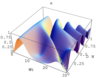
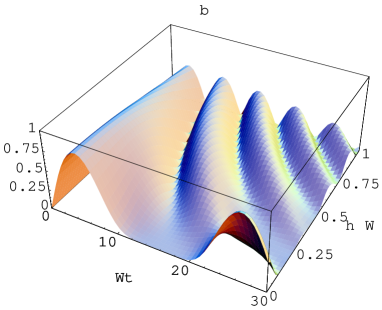
Figure 3: The entanglement $E_{\rho}\left(t\right)$ as a function of $\Omega t$ and $\Delta/\Omega$ ($\eta/\Omega)$. The parameters used in these figures are (a) $\phi=0,\eta/\Omega=0.1$ and $\Gamma=0,$ (b) $\Delta/\Omega=0$, and $\Gamma=0.$

For a very small value of $\eta$ (say $\eta=0.01)$, the situation becomes surprisingly interesting, at the initial period of the interaction time the entanglement is strong between the two quantum dots, but as the time goes on we have seen long survival of the disentanglement. This result indicates that the quantum dots will return to a pure state and completely disentangle from each other for a long period of the interaction time ($12\leq\Omega t\leq 19$). Finally, we may say that, it is possible to obtain a long surviving disentanglement using small values of inter-dot process hopping rate. Which means that the inter-dot process hopping rate plays an important role in the quantum entanglement.

An interesting question is whether or not the entanglement is affected by different values of the decoherence parameter $\Gamma/\Omega$. Figure 4a displays the effect of $\Gamma/\Omega$ on the entanglement, where $\Gamma/\Omega=0.01$. Evidently the evolution dynamics of $E_{\rho}\left(t\right)$ is sensitive to changes in the decoherence parameter $\Gamma/\Omega$. In the long time limit, the two quantum dots will be damped into their vacuum state due to the decoherence effect and entanglement decays to zero. Which means that the decoherence plays an important role in the reduction of the degree of entanglement. If the decoherence parameter is increased further, for the system with fixed values of the inter-dot coupling, the decrease in the amount of entanglement is faster (see figure 4b). It is likely that future source improvements will give values close to those expected for different initial states: the laser-dot coupling must be reduced to obtain sufficient entanglement to generate maximum entangled states. The oscillations in degree of entanglement between the quantum dots quickly damp out with an increase in $\Gamma/\Omega$. The subsystems will disentangle from each other and the steady state is reached at earlier interaction time. The change in $(\eta/\Omega)$ does not show much effect in the general structure of the degree of entanglement in contrast to the case $\Gamma=0$

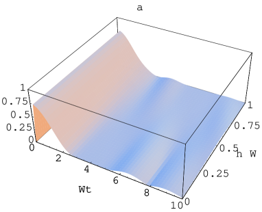
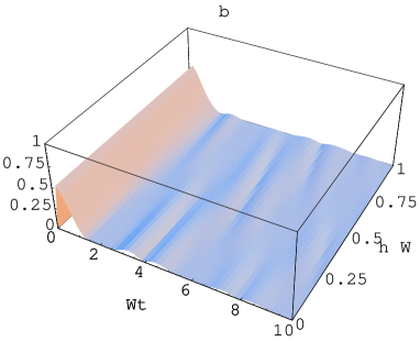
Figure 4: The entanglement $E_{\rho}\left(t\right)$ as a function of $\Omega t$ and $\eta/\Omega$. The parameters used in these figures are (a) $\Delta/\Omega=0$, and $\Gamma/\Omega=0.01$ and (b) $\Delta/\Omega=0$ and $\Gamma/\Omega=0.05.$

It would be also worthwhile to use different initial states setting, which would strongly help in creating the maximum entangled states. In a recent experimental work [36], it has been demonstrated that quantum superpositions and entanglement can be surprisingly robust.  This adds to the growing experimental evidence that robust manipulation of entanglement is feasible [38] with today’s technology. Entangling many degrees of freedom, or equivalently many qubits (quantum dots), remains a challenge, however, these experimental results are encouraging [36]. Also, in connection to the foundations of quantum theory, a deeper understanding of entanglement decoherence is expected to lead to new insights into the foundations of quantum mechanics  [37].

The remaining task is to identify and compare the results presented above for the entanglement degree with another accepted entanglement measure such as the concurrence [39]. One, possibly not very surprising, principal observation is that the numerical calculations corresponding to the same parameters, which have been considered above, give nearly the same behavior. This means that estimating the entanglement either using the negativity or concurrence measures gives qualitatively the same results.

5 Conclusion

We presented an analytical treatment for performing a maximum entangled states between two qubits in adjacent semiconductor quantum dots, formed through the interdot Förster interaction. The developed approach is capable of providing exact solutions to a class of problems which have only been treated approximately through previous studies. An important aspect is the insight gained by the possibility to combine the exact solution with the numerical treatments to generate maximum entangled states. More explicitly, in the exciton system, the large values of the detuning helps in generating maximum entangled states.  Nevertheless, the calculations indicate the maximum entangled states can still exist, even for the resonant case, when the electron and hole are driven by a suitable laser field (weak field limit).

We have extended our studies by giving an analysis and explanation of the predicted entanglement taking into account the decoherence effect. A remarkable property of the decoherence effect is that entanglement can fall abruptly to zero for a very long time and the entanglement will not be recovered i.e. the state will stay in the disentanglement separable state. Needless to say, there is still much work to be done and technical and general questions to be addressed: in particular, sources of three and four entangled quanta have very recently been reported [40], which in turn allows one to extend the question beyond two quantum dots to many-particle systems. This is also an exciting area for future study, both theoretically and experimentally.

Acknowledgments: We are grateful to the referees for very constructive comments and for suggesting various improvements in the manuscript. Also, we would like to thank E. Paspalakis for stimulating communications.

References

- [1] T. Brandes, Phys. Rep. 408, 315 (2005)
- [2] E. Paspalakis and A. F. Terzis, Phys. Lett. A 350, 396 (2006)
- [3] J. Gea-Banacloche, M. Mumba, and M. Xiao, Phys. Rev. B 74, 165330 (2006)
- [4] R. M. Stevenson, R. J. Young, P. See, D. G. Gevaux, K. Cooper, P. Atkinson, I. Farrer, D. A. Ritchie and A. J. Shields, Phys. Rev. B 73, 033306 (2006)
- [5] D. Loss and D.P. DiVincenzo, Phys. Rev. A 57, 120 (1998); Y.H. Shih and C.O. Alley, Phys. Rev. Lett. 61, 2921 (1988); X. X. Yi, G. R. Jin, and D. L. Zhou, Phys. Rev. A 63, 062307 (2001)
- [6] G. Chen, N.H. Bonadeo, D.G. Steel, D. Ganmon, D.S. Datzer, D. Park, and L.J. Sham, Science 289, 1906 (2000).
- [7] J.H. Reina, L. Quiroga, and N.F. Johnson, Phys. Rev. A 62, 012305 (2000); Y.-x. Liu, S. K. Özdemir, M. Koashi and N. Imoto, Phys. Rev. A 65, 042326 (2002).
- [8] W.G. van der Wiel, S. De Franceschi, J.M. Elzerman, T. Fujisawa, S. Tarucha, L.P. Kouwenhoven, Rev. Mod. Phys. 75, 1 (2003).
- [9] Z.-B. He, Y.-J. Xiong, Phys. Lett. A 349, 276 (2006).
- [10] W. Pötz, Appl. Phys. Lett. 71, 395 (1997); Phys. Rev. Lett. 79, 3262 (1997).
- [11] U. Hohenester, F. Rossi, and E. Molinari, Solid State Commun. 111, 187 (1999); N.H. Bonadeo, J. Erland, D. Gammon, D.S. Katzer, D. Park, and D.G. Steel, Science 282, 1473 (1998); Y. Toda, T. Sugimoto, M. Nishioka, and Y. Arakawa, Appl. Phys. Lett. 76, 3887 (2000).
- [12] E. Biolatti, R.C. Iotti, P. Zanardi, and F. Rossi, Phys. Rev. Lett. 85, 5647 (2000)
- [13] B. W. Lovett, J.H. Reina, A. Nazir, and G.A.D. Briggs, Phys. Rev. B 68, 205319 (2003)
- [14] W. Yin, J. Q. Liang and Q. W. Yan, J. Phys.: Condens. Matter 18, 9975 (2006)
- [15] R. S. Said, M. R. B. Wahiddin and B. A. Umarov, J. Phys. B: At. Mol. Opt. Phys. 39, 1269 (2006).
- [16] A. Nazir, B.W. Lovett, S.D. Barrett, T.P. Spiller, G.A.D. Briggs, Phys. Rev. Lett. 93, 150502 (2004) .
- [17] E. Paspalakis, Phys. Rev. B 67, 233306 (2003).
- [18] M. A. Nielsen and I. L. Chuang, Quantum Computation and Quantum Information (Cambridge University Press, Cambridge, 2000).
- [19] A. Olaya-Castro and N. F. Johnson, ”Handbook of Theoretical and Computational Nanotechnology” ed. M. Rieth and W. Schommers, American Scientific Publishers, 2006.
- [20] B. E. Kane, Nature 393, 133 (1998).
- [21] R. Vrijen, E. Yablonovitch, K. Wang, H. W. Jiang, A. Balandin, V. Roychowdhury, T. Mor, and D. DiVincenzo, Phys. Rev. A 62, 012306 (2000).
- [22] F.J. Rodrıguez, L. Quiroga, and N.F. Johnson, Phys. Rev. B 66, 161302(R) (2001).
- [23] Z. Kis and E. Paspalakis, J. Appl. Phys. 96, 3435-3439 (2004).
- [24] P. Zhang, C. K. Chan, Qi-Kun Xue and X.-G. Zhao, Phys. Rev. A 67, 012312 (2003).
- [25] J. H. Mc-Guire, K. K. Shakov and K. Y. Rakhimov, J. Phys. B: At. Mol. Opt. Phys. 36, 3145 (2003).
- [26] H. Moya-Cessa, Phys. Rep. 432, 1 (2006); H.-P. Breuer and F. Petruccione The theory of open quantum systems, Oxford University Press, Oxford, (2002)
- [27] T. Takagahara, Phys. Rev. B 60, 2638 (1999), T. Kuhn: in ”Theory of Trnasport Praperties of Semiconductor Nanostructuers”, ed E. Schőll (Hall a Chapman London 1999) p 173 and see alos G. Bukard, D. Loss and D.P. DiVincezo, Phys Rev. B 59, 2070 (1999).
- [28] X.X. Yi, C. Li, and J.C. Su, Phys. Rev. A 62, 013819 (2000)
- [29] L. Quiroga and N.F. Johnson, Phys. Rev. Lett. 83, 2270 (1999).
- [30] F.J. Rodriguez, L. Quiroga and N. F. Johnson, Phys. Stat. Sol. A 178, 403 (2000) and K. Kuroda et al J. Luminscence 122-123, 789 (2007).
- [31] A. Peres, Phys. Rev. Lett. 77, 1413 (1996).
- [32] M. Horodecki, P. Horodecki, and R. Horodecki, Phys. Lett. A 223, 1 (1996)
- [33] J. Lee and M. S. Kim, Phys. Rev. Lett. 84, 4236 (2000).
- [34] J. Lee, M. S. Kim, Y. J. Park and S. Lee, J. Mod. Opt. 47, 2151 (2000).
- [35] A. Messikh, Z. Ficek and M. R. B. Wahiddin, J. Opt. B: Quantum Semiclass. Opt. 5, L1 (2003); L. Zhou, H. S. Song and C. Li, J. Opt. B: Quantum Semiclass. Opt. 4, 425 (2002)
- [36] S. Fasel, M. Halder, N. Gisin and H. Zbinden, New J. Phys. 8, 13 (2006)
- [37] N. Gisin, Phys Lett A 210, 151 (1996); T. Yu and J. H. Eberly, Phys. Rev. B 68,165322 (2003).
- [38] R. T. Thew, A. Acın, H. Zbinden and N. Gisin, Phys. Rev. Lett. 93, 010503 (2004); D. N. Matsukevich, Phys. Rev. Lett. 95, 040405 (2005); R. T. Thew, S. Tanzilli, W. Tittel, H. Zbinden and N. Gisin, Phys. Rev. A 66, 062304 (2002); G. Ribordy, J.-D. Gautier, N. Gisin, O. Guinnard and H. Zbinden, J. Mod. Opt. 47, 517 (2000)
- [39] F. Mintert and A. Buchleitner, Phys. Rev. A 72, 012336 (2005)
- [40] P. Walther, J.-W. Pan, M. Aspelmeyer, R. Ursin, S. Gasparoni, A. Zeilinger, Nature 429, 158 (2004); M. W. Mitchell, J. S. Lundeen, and A. M. Steinberg, Nature 429, 161 (2004)