Azimuthal decorrelation of forward jets in Deep Inelastic Scattering

Abstract

We study the azimuthal angle decorrelation of forward jets in Deep Inelastic Scattering. We make predictions for this observable at HERA describing the high energy limit of the relevant scattering amplitudes with quasi–multi–Regge kinematics together with a collinearly improved evolution kernel for multiparton emissions.

CERN–PH–TH/2007–130
DESY–07–113

1 Introduction

In previous publications [1, 2, 3] we have studied the azimuthal angle decorrelation between Mueller–Navelet jets at different hadron colliders within the Balitsky–Fadin–Kuraev–Lipatov (BFKL) formalism [4] beyond leading order accuracy [5]. In the present work we extend these studies to predict the decorrelation in azimuthal angle between the electron and a forward jet associated to the proton in Deep Inelastic Scattering (DIS). When the separation in rapidity space, $Y$, between the scattered electron and the forward jet is large and the transverse momentum of the jet is similar to the virtuality of the photon resolving the hadron, then the dominant terms in the scattering amplitude are of the form $\sim(\alpha_{s}Y)^{n}$. These terms can be resummed to all orders by means of the BFKL integral equation. The calculation for this process is very similar to that of Mueller–Navelet jets, the only difference being the substitution of one jet vertex by a vertex describing the coupling of the electron to the NLO BFKL gluon Green’s function via a quark–antiquark pair.

This observable was previously investigated in the leading logarithmic approximation (LO) in Ref. [6]. In the following we build on that work while still using the LO approximation for the jet vertex and the virtual photon impact factor. However, we improve the calculation by considering the BFKL kernel to next–to–leading (NLO) accuracy, i.e. we also keep $\sim\alpha_{s}(\alpha_{s}Y)^{n}$ terms in the gluon Green’s function, a process–independent quantity which governs the dependence on $Y$ of the cross section, previous analysis in this direction can be found in Ref. [7]. The NLO terms in the impact factors should be relevant only in the regions of moderate $Y$, to include them in our analysis one could use Ref. [8] for the leptonic part and Ref. [9] for the forward jet vertex. We will leave this task for future work.

2 Forward jet cross section

For the production of a forward jet in DIS it is necessary to extract a parton with a large longitudinal momentum fraction $x_{\rm FJ}$ from the proton. When the jet is characterized by a hard scale it is possible to use conventional collinear factorization to describe the process. Consequently, the jet production rate may be written as

$$\sigma(s)=\int dx_{\rm FJ}\;f_{\rm eff}(x_{\rm FJ},\mu_{F}^{2})\hat{\sigma}(\hat{s}),$$ (1)

with $\hat{\sigma}(\hat{s})$ denoting the partonic cross section, and the effective parton density [10] being

$$f_{\rm eff}(x,\mu_{F}^{2})=G(x,\mu_{F}^{2})+\frac{4}{9}\sum_{f}\left[Q_{f}(x,\mu_{F}^{2})+\bar{Q}_{f}(x,\mu_{F}^{2})\right],$$ (2)

where the sum runs over all quark flavors, and $\mu_{F}$ stands for the factorization scale.

At partonic level we show a typical configuration contributing to $\hat{\sigma}(\hat{s})$ in Fig. 1. At the leptonic vertex, we treat the quark–antiquark pair inclusively, while we focus on the outgoing electron, which carries momentum $k_{1}$, and the gluon, which couples to the Green’s function with momentum $q_{1}$. In our notation the azimuthal angle of $k_{1}$ is $\alpha_{1}$ and that of $q_{1}$ is $\theta_{1}$.

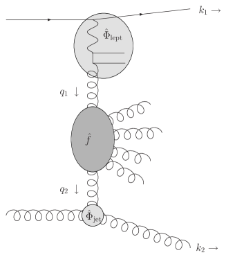
Figure 1: Kinematics of the partonic cross section.

We also work with commonly used DIS variables such as the proton momentum $P$, the photon’s momentum $q_{\gamma}$, its virtuality $Q^{2}=-q_{\gamma}^{2}$, the Bjorken scaling variable $x_{\rm Bj}=\frac{Q^{2}}{2Pq_{\gamma}}$ and the inelasticity $y=\frac{Pq_{\gamma}}{P(q_{\gamma}+k_{1})}$. Making use of the relation ${\bf k}_{1}^{2}=(1-y)Q^{2}$ and the specific structure of the leptonic vertex, we can write the partonic cross section in the form

$$\hat{\sigma}(\hat{s}) = \frac{\pi^{2}\bar{\alpha}_{s}^{2}}{2}\int d^{2}{{\bf k}_{1}}\int d^{2}{{\bf k}_{2}}\int\frac{d\omega}{2\pi i}e^{\omega Y}\langle{\bf k}_{1}|\hat{\Phi}_{\rm leptonic}\hat{f}_{\omega}\hat{\Phi}_{\rm jet}|{\bf k}_{2}\rangle$$ (3)

where the rapidity is defined as $Y=\ln x_{\rm FJ}/x_{\rm Bj}$. In bold we denote the transverse Euclidean momenta. We can further decompose the integration and write

$$\hat{\sigma}(\hat{s}) = \frac{\pi^{2}\bar{\alpha}_{s}^{2}}{2}\sum_{n,n^{\prime}=-\infty}^{\infty}\int d\alpha_{1}\int dy\int d^{2}{{\bf k}_{2}}\int\frac{d\omega}{2\pi i}\int d^{2}{{\bf q}_{1}}\int d^{2}{{\bf q}_{2}}\int d\nu\int d\nu^{\prime}$$ (4)

$$\times\langle y,\alpha_{1}|\hat{\Phi}_{\rm leptonic}|{\bf q}_{1}\rangle\langle{\bf q}_{1}|\nu,n\rangle\langle n,\nu|\hat{f}_{\omega}|\nu^{\prime},n^{\prime}\rangle\langle n^{\prime},\nu^{\prime}|{\bf q}_{2}\rangle\langle{\bf q}_{2}|\hat{\Phi}_{\rm jet}|{\bf k}_{2}\rangle e^{\omega Y}.$$

We have introduced a Fourier expansion on conformal spins $n$, to be defined below. The integrals in transverse momenta are taken over the whole two dimensional space while the $\nu$ integrations go from $-\infty$ to $\infty$. The contour in the $\omega$–plane is to be taken to the right of all possible singularities.

In Eq. (4) we have used the transverse momentum representation defined by

$$\hat{\bf q}_{1}|{\bf q}_{1}\rangle= {\bf q}_{1}|{\bf q}_{1}\rangle \langle{\bf q}_{1}|{\bf q}_{2}\rangle= \delta^{(2)}\left({\bf q}_{1}-{\bf q}_{2}\right),$$ (5)

where the kernel in operator form $\hat{\mathcal{K}}$,

$$\mathcal{K}({\bf q}_{1},{\bf q}_{2})=\langle{\bf q}_{1}|\hat{\mathcal{K}}|{\bf q}_{2}\rangle,$$ (6)

defines the BFKL integral equation at NLO, i.e.,

$$\omega\,\hat{f}_{\omega}= \hat{1}+\hat{\mathcal{K}}\hat{f}_{\omega}.$$ (7)

To change representation we introduce the basis

$$\langle{\bf q}_{1}|\nu,n\rangle=\frac{1}{\pi\sqrt{2}}\left({\bf q}_{1}^{2}\right)^{i\nu-\frac{1}{2}}e^{in\theta_{1}},$$ (8)

where $\theta_{1}$ is the azimuthal angle of ${\bf q}_{1}$. The normalization in this new basis reads

$$\langle n^{\prime},\nu^{\prime}|\nu,n\rangle=\int d^{2}{{\bf q}_{1}}\frac{1}{2\pi^{2}}\left({\bf q}_{1}^{2}\right)^{i(\nu-\nu^{\prime})-1}e^{i(n-n^{\prime})\theta}=\delta(\nu-\nu^{\prime})\delta_{nn^{\prime}}.$$ (9)

In this $|n,\nu\rangle$ representation the eigenstates of the LO kernel are

$$\hat{\mathcal{K}}_{0}|\nu,n\rangle=\bar{\alpha}_{s}\chi_{0}\left(|n|,\frac{1}{2}+i\nu\right)|\nu,n\rangle,$$ (10)

with $\bar{\alpha}_{s}=\alpha_{s}N_{c}/\pi$ and

$$\chi_{0}(n,\gamma)=2\psi(1)-\psi\left(\gamma+\frac{n}{2}\right)-\psi\left(1-\gamma+\frac{n}{2}\right),$$ (11)

where $\psi(x)=\Gamma^{\prime}(x)/\Gamma(x)$, with $\Gamma$ being the Euler gamma function.

Unfortunately, to the best of our knowledge, the azimuthal angle correlation between the electron and a forward jet has not been extracted from the HERA data so far. For a future comparison with the experimental results in this work we implement the same kinematical cuts and constraints as those used at HERA. The ZEUS [11] and H1 [12] collaborations have imposed upper and lower cuts in the transverse momentum of the forward jet taking into account the photon virtuality $Q^{2}$. They performed these cuts in order to ensure that both ends of the gluon ladder have a similar characteristic transverse scale. More in detail, they imposed

$${\rm ZEUS:} \frac{1}{2}<\frac{{\bf k}_{2}^{2}}{Q^{2}}<2,$$ (12a)

$${\rm H1:} \frac{1}{2}<\frac{{\bf k}_{2}^{2}}{Q^{2}}<5.$$ (12b)

These requirements are intended to suppress DGLAP evolution without affecting the BFKL dynamics. The implementation in our jet vertex of these constraints is straightforward. For the ZEUS condition we have

$$\frac{1}{2}\int d{\bf k}_{2}^{2}\int d^{2}{{\bf q}_{2}}\;\langle n^{\prime},\nu^{\prime}|{\bf q}_{2}\rangle\langle{\bf q}_{2}|{\hat{\Phi}_{\rm jet}}|{\bf k}_{2}\rangle\\ =:c_{2}(\nu^{\prime})\frac{e^{-in^{\prime}\alpha_{2}}}{2\pi}=\frac{1}{\sqrt{2}}\frac{1}{\frac{1}{2}+i\nu^{\prime}}\left(\frac{Q^{2}}{2}\right)^{-i\nu^{\prime}-\frac{1}{2}}\left[1-\left(\frac{1}{4}\right)^{i\nu^{\prime}-\frac{1}{2}}\right]\frac{e^{-in^{\prime}\alpha_{2}}}{2\pi}.$$ (13)

In the case of the H1 condition the $1/4$ should be replaced for a $1/10$. For simplicity, in the following, we follow the ZEUS cut.

In Ref. [6] it was shown that the leptonic vertex, in our notation, reads

$$\langle y,\alpha_{1}|\hat{\Phi}_{\rm leptonic}|{\bf q}_{1}\rangle$$

$$= \int dQ^{2}\frac{4\alpha^{2}}{\pi^{2}N_{c}\;y\,Q^{2}}\sum_{q}e_{q}^{2}\int_{0}^{1}\int_{0}^{1}\frac{d\xi\,d\zeta}{\xi(1-\xi)Q^{2}+\zeta(1-\zeta){\bf q}_{1}^{2}}$$

$$\times\Bigg{\{}\left(\frac{1}{2}-\xi(1-\xi)-\zeta(1-\zeta)+2\xi(1-\xi)\zeta(1-\zeta)\right)y^{2}$$

$$\phantom{\times\Bigg{\{}}+\Big{(}1-2\xi(1-\xi)-2\zeta(1-\zeta)+12\xi(1-\xi)\zeta(1-\zeta)\Big{)}(1-y)$$

$$\phantom{\times\Bigg{\{}}-4\xi(1-\xi)\zeta(1-\zeta)(1-y)\cos\big{(}2(\theta_{1}-\alpha_{1})\big{)}\Bigg{\}}$$

$$=: \int dQ^{2}\left[2a_{1}^{(0)}({\bf q}_{1}^{2},y,Q^{2})+2a_{1}^{(2)}({\bf q}_{1}^{2},y,Q^{2})\cos\big{(}2(\theta_{1}-\alpha_{1})\big{)}\right],$$ (14)

where $\alpha$ denotes the electromagnetic fine structure constant and $\sum_{q}e_{q}^{2}$ is the sum over the electric charges of the produced quark–antiquark pairs.

To construct our cross sections we need to find the projection of this leptonic impact factor onto the $|\nu,n\rangle$ basis. We obtained

$$\int d^{2}{{\bf q}_{1}}\langle y,\alpha_{1}|\hat{\Phi}_{\rm leptonic}|{\bf q}_{1}\rangle\langle{\bf q}_{1}|\nu,n\rangle$$

$$= \int dQ^{2}\left[2A_{1}^{(0)}\left(\nu,y,Q^{2}\right)+A_{1}^{(2)}\left(\nu,y,Q^{2}\right)\left(\delta_{n,-2}e^{-2i\alpha_{1}}+\delta_{n,2}e^{2i\alpha_{1}}\right)\right],$$ (15)

with

$$A_{1}^{(n)}\left(\nu,y,Q^{2}\right)=\frac{1}{\sqrt{2}}\int d{\bf q}_{1}^{2}\;a_{1}^{(n)}({\bf q}_{1}^{2},y,Q^{2})\left({\bf q}_{1}^{2}\right)^{i\nu-\frac{1}{2}}.$$ (16)

To calculate these coefficients we need integrals of the type

$$\int_{0}^{1}d\xi\,(\xi(1-\xi))^{t_{\xi}}\int_{0}^{1}d\zeta\,(\zeta(1-\zeta))^{t_{\zeta}}\int_{0}^{\infty}d{\bf q}_{1}^{2}\frac{\left({\bf q}_{1}^{2}\right)^{i\nu-\frac{1}{2}}}{\xi(1-\xi)Q^{2}+\zeta(1-\zeta){\bf q}_{1}^{2}}=\\ \frac{\pi\left(Q^{2}\right)^{i\nu-\frac{1}{2}}}{\cosh(\pi\nu)}B\left(\frac{1}{2}+t_{\xi}+i\nu,\frac{1}{2}+t_{\xi}+i\nu\right)B\left(\frac{1}{2}+t_{\zeta}-i\nu,\frac{1}{2}+t_{\zeta}-i\nu\right),$$ (17)

with $B$ representing the Euler beta function. Using this formula for $t_{\xi/\zeta}\in\{0,1\}$ we obtained

$$A_{1}^{(0)}\left(\nu,y,Q^{2}\right)= \phantom{\times}\frac{\alpha^{2}\sqrt{2}}{y\,N_{c}}\left(Q^{2}\right)^{i\nu-\frac{1}{2}}\sum_{q}e_{q}^{2}\frac{1}{16\nu(\nu^{2}+1)}\frac{\tanh(\pi\nu)}{\cosh(\pi\nu)}$$

$$\times\left(\frac{4\nu^{2}+9}{2}y^{2}+(12\nu^{2}+11)(1-y)\right),$$ (18a)

$$A_{1}^{(2)}\left(\nu,y,Q^{2}\right)= \phantom{\times}\frac{\alpha^{2}\sqrt{2}}{y\,N_{c}}\left(Q^{2}\right)^{i\nu-\frac{1}{2}}\sum_{q}e_{q}^{2}\frac{1}{16\nu(\nu^{2}+1)}\frac{\tanh(\pi\nu)}{\cosh(\pi\nu)}$$

$$\times\left(-(4\nu^{2}+1)(1-y)\right).$$ (18b)

The last piece needed to complete Eq. (4) is the gluon Green’s function, which can be written as

$$\langle n,\nu|\hat{f}|\nu^{\prime},n^{\prime}\rangle=\int\frac{d\omega}{2\pi i}\,\langle n,\nu|\hat{f}_{\omega}|\nu^{\prime},n^{\prime}\rangle e^{\omega Y}=e^{\chi\left(|n|,\frac{1}{2}+i\nu,\bar{\alpha}_{s}\right)Y}\;\delta(\nu-\nu^{\prime})\delta_{nn^{\prime}},$$ (19)

with the eigenvalue of the BFKL kernel being

$$\chi\Big{(}n,\frac{1}{2}+i\nu,\bar{\alpha}_{s}\Big{)}=\bar{\alpha}_{s}\chi_{0}\Big{(}n,\frac{1}{2}+i\nu\Big{)}\\ +\bar{\alpha}_{s}^{2}\left(\chi_{1}\Big{(}n,\frac{1}{2}+i\nu\Big{)}-\frac{\beta_{0}}{8N_{c}}\chi_{0}\Big{(}n,\frac{1}{2}+i\nu\Big{)}h_{\rm rc}^{(n)}\left(\nu,y,Q^{2}\right)\right).$$ (20)

The action of the scale invariant sector of the NLO correction, given by the function $\chi_{1}(n,\gamma)$, was calculated in Ref. [13]. The last term in this equation stems from the scale dependent part of the NLO kernel, i.e. from the running of the coupling. Its explicit form, in our representation, depends on the impact factors as given below and is discussed in more detail in Refs. [1, 3].

$$h_{\rm rc}^{(0)}\left(\nu,y,Q^{2}\right)= -\frac{1}{2\nu^{2}+\frac{1}{2}}+\frac{3\ln(2)}{5-4\cos(\nu\,\ln 4)}$$

$$-i\Bigg{[}\pi\frac{\cosh(2\pi\nu)-3}{\sinh(2\pi\nu)}+\frac{4\sin(\nu\,\ln 4)\ln(2)}{5-4\cos(\nu\,\ln 4)}$$

$$\hphantom{-i\Bigg{[}}-8\nu\frac{y^{2}+6(1-y)}{9y^{2}+22(1-y)+4(y^{2}+6(1-y))\nu^{2}}$$

$$\hphantom{-i\Bigg{[}}+\frac{3\nu^{2}+1}{\nu(\nu^{2}+1)}-\frac{\nu}{\nu^{2}+\frac{1}{4}}\Bigg{]},$$ (21a)

$$h_{\rm rc}^{(2)}\left(\nu,y,Q^{2}\right)= -\frac{1}{2\nu^{2}+\frac{1}{2}}+\frac{3\ln(2)}{5-4\cos(\nu\,\ln 4)}$$

$$-i\Bigg{[}\pi\frac{\cosh(2\pi\nu)-3}{\sinh(2\pi\nu)}+\frac{4\sin(\nu\,\ln 4)\ln(2)}{5-4\cos(\nu\,\ln 4)}$$

$$\hphantom{-i\Bigg{[}}+\frac{3\nu^{2}+1}{\nu(\nu^{2}+1)}-\frac{3\nu}{\nu^{2}+\frac{1}{4}}\Bigg{]}.$$ (21b)

Blending together the leptonic vertex of Eq. (15), the Green’s function of Eq. (19) and the forward jet vertex given in Eq. (13), we obtain the cross section of Eq. (4), which can be expressed in differential form as

$$\frac{d\hat{\sigma}}{dy\,dQ^{2}\,d\phi}=\frac{\pi^{2}\bar{\alpha}_{s}^{2}}{2}\int d\nu\int d\nu^{\prime}\Bigg{[}A_{1}^{(0)}\left(\nu,y,Q^{2}\right)\langle 0,\nu|\hat{f}|\nu^{\prime},0\rangle c_{2}(\nu^{\prime})\\ +A_{1}^{(2)}\left(\nu,y,Q^{2}\right)\langle 2,\nu|\hat{f}|\nu^{\prime},2\rangle c_{2}(\nu^{\prime})\cos\,2\phi\Bigg{]},$$ (22)

where we have introduced the azimuthal angle $\phi=\alpha_{2}-\alpha_{1}$ between the electron and the forward jet. We have also made use of the relation $\langle n,\nu|\hat{f}|\nu^{\prime},n\rangle=\langle-n,\nu|\hat{f}|\nu^{\prime},-n\rangle$.

It is more convenient to write Eq. (22) as

$$\frac{d\hat{\sigma}}{d\phi\;dy\;dQ^{2}}=\frac{\pi^{2}\bar{\alpha}_{s}^{2}}{2}\left[B^{(0)}\left(y,Q^{2},Y\right)+B^{(2)}\left(y,Q^{2},Y\right)\cos 2\phi\right],$$ (23)

where the coefficients $B^{(n)}$ at LO read

$$B^{(n)}_{\rm LO}\left(y,Q^{2},Y\right)=\int d\nu\;A^{(n)}\left(\nu,y,Q^{2}\right)\,c_{2}(\nu)e^{Y\bar{\alpha}_{s}\chi_{0}\left(\left|n\right|,\nu\right)},$$ (24)

and at NLO:

$$B^{(n)}_{\rm NLO}\left(y,Q^{2},Y\right)=\int d\nu\;A^{(n)}\left(\nu,y,Q^{2}\right)\,c_{2}(\nu)\\ \times e^{{\bar{\alpha}}_{s}(Q^{2}){\rm Y}\left(\chi_{0}\left(\left|n\right|,\nu\right)+{\bar{\alpha}}_{s}(Q^{2})\left(\chi_{1}\left(\left|n\right|,\nu\right)-\frac{\beta_{0}}{8N_{c}}\chi_{0}(n,\frac{1}{2}+i\nu)h_{\rm rc}^{(n)}(\nu,y,Q^{2})\right)\right)}.$$ (25)

The BFKL resummation presents an instability in transverse momentum space when the NLO corrections are taken into account [14]. A prescription to increase the convergence of the perturbative expansion is to improve the original calculation by imposing compatibility of the scattering amplitudes with the collinear limit dominated by renormalization group evolution [15, 16]. In recent publications [2, 3] we have introduced these collinear improvements to describe azimuthal angle dependences in the context of Mueller–Navelet jets. Our results were later on reproduced in Ref. [17].

From a technical point of view, the collinearly–improved kernel of Ref. [2] differs from the one needed in the DIS case only in the term due to the running of the coupling in Eq. (20). This contribution changes the single and double poles of the original kernel in the form

$$a_{0}\quad\rightarrow\quad a_{0}-\frac{\beta_{0}}{8N_{c}}\left(\frac{7}{6}+\frac{1-y}{y\left(\frac{y}{2}-1\right)+1}\right),$$ (26)

$$a_{2}\quad\rightarrow\quad a_{2}-\frac{\beta_{0}}{8N_{c}}\left(\frac{107}{30}+\frac{5\ln 2}{3}\right),$$ (27)

$$b_{n}\quad\rightarrow\quad b_{n}+\frac{\beta_{0}}{4N_{c}}.$$ (28)

These equations hence replace Eqs. (24, 25) of Ref. [2].

3 Phenomenology

Besides the particular experimental cuts in the forward jet taken into account when calculating the jet vertex of Eq. (13), we also used the following experimentally motivated [18] constraints in the leptonic sector:

$$20~{}{\rm GeV}^{2}<Q^{2}<100~{}{\rm GeV}^{2},$$

$$0.05<y<0.7,$$

$$5\cdot 10^{-3}>x_{\rm Bj}>4\cdot 10^{-4}.$$ (29)

The final expression for the cross section at hadronic level reads

$$\frac{d\sigma}{dY\;d\phi}=:C_{0}(Y)+C_{2}(Y)\cos 2\phi,$$ (30)

with

$$C_{n}(Y)=\frac{\pi^{2}\bar{\alpha}_{s}^{2}}{2}\int_{\rm cuts}dx_{\rm FJ}\,dQ^{2}\,dy\,f_{\rm eff}(x_{\rm FJ},Q^{2})B^{(n)}(y,Q^{2},Y)\delta\left(x_{\rm FJ}-\frac{Q^{2}e^{Y}}{ys}\right),$$ (31)

where we performed the convolution with the effective parton distribution of Eq. (2). The index in the integral sign refers to the particular cuts of Eq. (29). The integration over the longitudinal momentum fraction $x_{\rm FJ}$ of the forward jet involves a delta function fixing the rapidity $Y=\ln x_{\rm FJ}/x_{\rm Bj}$. It is noteworthy that any additional experimental upper cut on $x_{\rm FJ}$ would modify the coefficients $C_{n}$, with a negligible change in their ratios.

Since the structure of the electron vertex singles out the components with conformal spin 0 and 2, the number of observables related to the azimuthal angle dependence is limited when compared to the Mueller–Navelet case. The most relevant observable is the dependence of the average $<\cos 2\phi>=C_{2}/C_{0}$ with the rapidity difference between the forward jet and outgoing lepton. It is natural to expect that the forward jet will be more decorrelated from the leptonic system as the rapidity difference is larger since the phase space for further gluon emission opens up. This is indeed what we observe in our numerical results shown in Fig. 2. We find similar results to the Mueller–Navelet jets case where the most reliable calculation is that with a collinearly–improved kernel. The main effect of the higher order corrections is to increase the azimuthal angle correlation for a given rapidity difference, while keeping the decrease of the correlation as $Y$ grows.

Figure 2: $<\cos 2\phi>$ at the $ep$ collider HERA at leading (solid), next to leading order (dashed), and for resummed kernel (dash-dotted).

It is interesting to point out that, even for very small $Y$, the inclusive quark–antiquark pair (produced to couple the electron to the gluon evolution) generates in the case of no gluon emission some angular decorrelation between the forward jet and the electron.

Finally, we estimate the theoretical uncertainties derived from not including the NLO impact factors by varying the scale $s_{0}$, and those related to the running of the coupling by doing the same with the renormalization scale $\mu$. The range of variation in both parameters is between $1/2$ and 2 and the result is shown in Fig. 3.

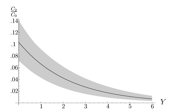
Figure 3: $<\cos 2\phi>$ at the $ep$ collider HERA for resummed kernel (dash-dotted). The gray band reflects the uncertainty in $s_{0}$ and in the renormalization scale $\mu$.

At present, the data taken at the HERA collider provide the only possibility to experimentally test our prediction. Nevertheless there are proposals to upgrade the Large Hadron Collider (LHC) at CERN to a Large Electron Hadron Collider [19]. The projected center of mass energy $\sqrt{s}=1.4~{}{\rm TeV}$ is more than four times bigger than at HERA and would allow for a larger rapidity separation between the electron and the forward jet. We use the same cuts as for HERA (Eq. (29)) apart from an adjusted lower bound for $x_{\rm Bj}$ of $2\cdot 10^{-5}$. Fig. 4 is a plot of our results, which are very similar to those presented in Fig. 3.

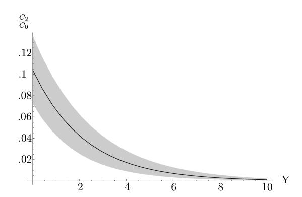
Figure 4: $<\cos 2\phi>$ at a possible $ep$ collider LHeC with a gray band reflecting the uncertainty in $s_{0}$ and in the renormalization scale $\mu$.

4 Conclusions

We have studied the effect of higher order corrections to the BFKL equation on the angular decorrelation of forward jets in Deep Inelastic Scattering. The effect of these additional terms is similar to the previously studied case of Mueller–Navelet jets at hadron colliders. As the rapidity difference between the outgoing lepton and the forward jet increases, the two systems decorrelate in azimuthal angle due to the extra emission of soft gluons and higher order terms largely increase the amount of correlation when compared to the leading order calculations. It would be very interesting to extract this dependence from the HERA data with forward jets and study how important BFKL effects are for this observable. If the experience at the Tevatron is valid in this case, the BFKL prediction will probably lie below the data, with a gradual improvement of the fits as the rapidity difference increases.

Acknowledgments

We would like to thank J. Bartels, D. Dobur, H. Jung, L. Motyka and J. Terrón for very interesting discussions. F.S. is supported by the Graduiertenkolleg “Zukünftige Entwicklungen in der Teilchenphysik”.

References

• [1] A. Sabio Vera, Nucl. Phys.  B 746 (2006) 1.
• [2] A. Sabio Vera and F. Schwennsen, Nucl. Phys.  B 776 (2007) 170.
• [3] F. Schwennsen, DESY-THESIS-2007-001, hep-ph/0703198.
• [4] V.S. Fadin, E.A. Kuraev and L.N. Lipatov, Phys. Lett. B60 (1975) 50; E.A. Kuraev, L.N. Lipatov and V.S. Fadin, Zh. Eksp. Teor. Fiz. 71 (1976) 840 [Sov. Phys. JETP 44 (1976) 443]; 72 (1977) 377 [45 (1977) 199]; Ya.Ya. Balitskii and L.N. Lipatov, Sov. J. Nucl. Phys. 28 (1978) 822.
• [5] V.S. Fadin and L.N. Lipatov, Phys. Lett. B429 (1998) 127; M. Ciafaloni and G. Camici, Phys. Lett. B430 (1998) 349.
• [6] J. Bartels, V. Del Duca, and M. Wusthoff, Z. Phys. C76, 75 (1997).
• [7] O. Kepka, C. Royon, C. Marquet and R. Peschanski, hep-ph/0609299, hep-ph/0612261.
• [8] J. Bartels, S. Gieseke and C. F. Qiao, Phys. Rev. D63, 056014 (2001); J. Bartels, S. Gieseke and A. Kyrieleis, Phys. Rev. D65, 014006 (2002); J. Bartels, D. Colferai, S. Gieseke and A. Kyrieleis, Phys. Rev. D66, 094017 (2002); J. Bartels and A. Kyrieleis, Phys. Rev. D70, 114003 (2004); G. Chachamis, DESY-THESIS-2006-031; V. S. Fadin, D. Y. Ivanov and M. I. Kotsky, Phys. Atom. Nucl. 65, 1513 (2002); V. S. Fadin, D. Y. Ivanov and M. I. Kotsky, Nucl. Phys. B658, 156 (2003).
• [9] J. Bartels, D. Colferai and G. P. Vacca, Eur. Phys. J.  C 24 (2002) 83; Eur. Phys. J.  C 29 (2003) 235.
• [10] B. L. Combridge and C. J. Maxwell, Nucl. Phys. B239, 429 (1984).
• [11] ZEUS, S. Chekanov et al., Phys. Lett. B632, 13 (2006).
• [12] H1, A. Aktas et al., Eur. Phys. J. C46, 27 (2006).
• [13] A. V. Kotikov and L. N. Lipatov, Nucl. Phys. B582, 19 (2000).
• [14] D. A. Ross, Phys. Lett. B431, 161 (1998).
• [15] G. P. Salam, JHEP 07, 019 (1998).
• [16] A. Sabio Vera, Nucl. Phys. B722, 65 (2005).
• [17] C. Marquet and C. Royon, arXiv:0704.3409.
• [18] D. Dobur, private communications.
• [19] J. B. Dainton, M. Klein, P. Newman, E. Perez and F. Willeke, JINST 1 (2006) P10001.