A census of metals and baryons in stars in the local Universe

Abstract

We combine stellar metallicity and stellar mass estimates for a large sample of galaxies drawn from the Sloan Digital Sky Survey Data Release Two (SDSS DR2) spanning wide ranges in physical properties, in order to derive an inventory of the total mass of metals and baryons locked up in stars in the local Universe. Physical parameter estimates are derived from galaxy spectra with high signal-to-noise (S/N) ratio (of at least 20). Coadded spectra of galaxies with similar velocity dispersions, absolute $r$-band magnitudes and 4000Å-break values are used for those regions of parameter space where individual spectra have lower S/N. We estimate the total density of metals $\rho_{Z}$ and of baryons $\rho_{\ast}$ in stars and, from these two quantities, we obtain a mass- and volume-averaged stellar metallicity of $\langle Z_{\ast}\rangle=1.04\pm 0.14~{}Z_{\odot}$, i.e. consistent with solar. We also study how metals are distributed in galaxies according to different properties, such as mass, morphology, mass- and light-weighted age, and we then compare these distributions with the corresponding distributions of stellar mass. We find that the bulk of metals locked up in stars in the local Universe reside in massive, bulge-dominated galaxies, with red colours and high 4000Å-break values corresponding to old stellar populations. Bulge-dominated and disc-dominated galaxies contribute similar amounts to the total stellar mass density, but have different fractional contributions to the mass density of metals in stars, in agreement with the mass-metallicity relation. Bulge-dominated galaxies contain roughly 40 percent of the total amount of metals in stars, while disc-dominated galaxies less than 25 percent. Finally, at a given galaxy stellar mass, we define two characteristic ages as the median of the distributions of mass and metals as a function of age. These characteristic ages decrease progressively from high-mass to low-mass galaxies, consistent with the high formation epochs of stars in massive galaxies.

1 Introduction

Constraining the star formation and chemical evolution histories of galaxies is one of the fundamental goals in observational cosmology. The evolution of the global star formation rate (SFR) has to map the evolution over cosmic time of its products, i.e. the baryonic and metal content of the Universe.

The most direct way to constrain the star formation and chemical evolution history over cosmic times is to trace back galaxy properties (star formation rate, metallicity, stellar mass) through observations at different redshifts. Several studies on the evolution of the rest-frame UV emission density of galaxies, converted into star formation or metal ejection rates, have converged into a picture in which the maximum of galaxy star formation activity occurs over the redshift range $1\la z\la 2$ and declines sharply from $z=1$ towards the present (Lilly et al., 1996; Connolly et al., 1997; Cowie et al., 1999). While several recent studies have built a consistent picture of the decline in cosmic star formation rate from $z\sim$1 to the present (e.g. Hopkins & Beacom, 2006, and references therein), more uncertain is the behaviour at redshift higher than 2, because of the poor understanding of the effect of dust on the SFR derived from UV Spectral Energy Distributions (SED) of high-redshift galaxies (Madau et al., 1996; Steidel et al., 1999; Ivison et al., 2002). A broad peak of high star formation over the redshift range $z\sim 1-2$ and then a rapid decline toward the present are features predicted (or reproduced) also by both chemical evolution models (Pei & Fall, 1995; Edmunds & Phillipps, 1997; Pei et al., 1999) and by semianalytic models of galaxy formation (e.g. Baugh et al., 1998).

A complementary approach is to study the chemical and star formation history over cosmic times through the so-called ‘fossil cosmology’, i.e. determining the past history of the Universe from its present contents. This approach has benefited from large spectroscopic surveys in the local Universe, such as the 2dF Galaxy Redshift Survey (2dFGRS, Colless et al., 2001) and the Sloan Digital Sky Survey (SDSS, York et al., 2000), which provide detailed spectral information for hundreds of thousands of galaxies. Based on such surveys, Baldry et al. (2002) and Glazebrook et al. (2003) have constrained the cosmic star formation history (SFH) from the ‘cosmic optical spectrum’, which represents the average emission from all the objects in a representative volume of the Universe and has the advantage of being fitted by simpler models of star formation histories than those needed for individual objects. Heavens et al. (2004) and Jimenez et al. (2005) have applied a data compression algorithm (MOPED, Heavens et al., 2000) to extract the SFH of $\sim 100,000$ SDSS DR1 galaxies from their optical spectra. This work has been recently extended to the SDSS DR3 (three times larger sample) by Panter et al. (2006), with improvements both in the data and in the modelling sides (see also Tojeiro et al. 2007, Ocvirk et al. 2006 and Cid Fernandes et al. 2007 for similar methods to recover stellar content and star formation histories from galaxy spectra). This allowed them to derive the cosmic SFH from the ‘fossil record’ and study it as a function of the present-day stellar mass of galaxies.

The contribution to the global SFR by galaxies of different mass is being studied not only in the local Universe but also at higher redshift. Juneau et al. (2005) studied the dependence of the cosmic SFH directly on the stellar mass at the epoch of observation over the redshift range $0.8<z<2$, based on a near-infrared selected sample from the Gemini Deep Deep Survey (GDDS, Abraham et al., 2004). Similarly, Bundy et al. (2005) have quantified the decrease with redshift of the mass limit above which star formation appears to be quenched, based on a sample of more than 8000 galaxies in the redshift range $0.4<z<1.4$ drawn from the DEEP2 Galaxy Redshift Survey (Davis et al., 2003). These results confirm those previously found by Brinchmann & Ellis (2000) for $0<z<1$. While high- and intermediate-mass galaxies have transitioned to a quiescent phase of star formation by $z\sim 1$, less massive systems dominate the star formation rate density till the present epoch. It appears, though, that the global star formation rate has been declining since $z\sim$1 for all galaxies populations, at a rate which is independent of stellar mass, as shown by Zheng et al. (2007) estimating SFRs of $\sim$15000 COMBO-17 galaxies from UV and IR luminosities and accounting for individually IR-undetectable galaxies (Zheng et al., 2006).

An important consistency check for all these studies comes from the comparison of the density of stellar mass and of metals at different epochs expected from the cosmic star formation and chemical enrichment histories (i.e. the integral of these histories) with those directly measured. The evolution of the global stellar mass density out to $z=3$ has been first determined by Dickinson et al. (2003). In concordance with estimates of the cosmic SFH, their study suggests that the redshift range $1<z<2.5$ is a critical epoch when galaxies are growing rapidly attaining their final stellar mass.

Much effort has been put also in measuring the chemical composition of galaxies at different epochs, through optical nebular emission lines studies at $z<1$ (e.g. Kobulnicky & Zaritsky, 1999; Lilly et al., 2003; Kobulnicky & Kewley, 2004; Ellison et al., 2005), through Lyman-break and UV-selected star-forming galaxies up to $z\sim 3$ (e.g. Pettini et al., 2001; Steidel et al., 2004; Shapley et al., 2004; Erb et al., 2006), through quasar absorption-line systems, in particular Damped Ly-$\alpha$ Absorbers (DLA) at any redshift (e.g. Pettini et al., 1994; Lanzetta et al., 1995; Pettini et al., 1997; Péroux et al., 2003, 2005; Péroux et al., 2006). All these studies have highlighted a shortfall of metals in observed galaxy populations with respect to expectations from the cosmic SFH, known as the ‘missing metals’ problem at redshift around 2.5 (Pettini, 2006; Bouché et al., 2005). A large fraction could be hosted in a recently discovered population of sub-DLAs (Péroux et al., 2005). Not more than $30-40$ percent seems to be in intergalactic medium (IGM), and probably $\la 35$ percent of metals is still ‘missing’ from the census (Bouché et al., 2007). These metals are likely locked in the hot gas phase (Ferrara et al., 2005; Davé & Oppenheimer, 2007). The present-day distribution of metals is still highly uncertain, because little is known about the chemical composition of the possibly dominant baryonic component, the warm hot intergalactic medium (WHIM). However the fraction of metals contained in galaxies, in particular those locked into the stellar component, has increased from $z\sim 2$ to the present, and is probably comparable to the fraction of metals outside galaxies (e.g. Dunne et al., 2003; Calura & Matteucci, 2004).

In this work we focus on the baryonic and metal content of the stellar component of galaxies in the local Universe. What is the total amount of metals and baryons locked up into stars by the present epoch? What is the resulting average stellar metallicity of the present-day Universe? To address these questions we join together information about the stellar mass and chemical properties of present-day galaxies, supported by the large statistics provided by the SDSS. The sample we analyse span large ranges in physical, spectral and morphological properties, and constitute in this sense a representative sample of the local Universe. This allows us also to study how metals and baryons are distributed among galaxies with different properties. In particular, we want to quantify the fraction of metals, in comparison to the fraction of baryons, locked up in galaxies as a function of their stellar mass, morphology and age.

We exploit new estimates of physical parameters, such as stellar metallicity and stellar mass, that we previously derived (Gallazzi et al., 2005, hereafter paper I) for a large sample of nearly $2\times 10^{5}$ galaxies drawn from the Sloan Digital Sky Survey Data Release Two (SDSS DR2). We include all galaxies types, from quiescent early-type to actively star-forming galaxies. In our previous works we focused only on galaxies with high signal-to-noise ratio (S/N) spectra, because of the poor constraints that can be obtained on stellar metallicity from low-S/N spectra. We circumvent here this problem by stacking individual spectra of low-S/N galaxies with similar properties in order to obtain high-S/N (average) spectra.

The sample analysed is described in Section 2.1, along with the stacking technique adopted in order to include galaxies with low-S/N spectra (Section 2.2). We illustrate the physical parameters estimates extracted from individual galaxy spectra and from coadded spectra in Section 2.3. In Section 3.1 we derive the mass density of baryons and of metals locked up in stars, expressed also in terms of the average stellar metallicity of the local Universe. We then discuss several sources of systematic uncertainties in Section 3.2 and compare with other estimates in the literature in Section 3.3. Section 4.1 provides an inventory of the stellar metallicity and stellar mass today, focusing on the characteristic age of the stellar mass and metallicity distributions in Section 4.2. We compare the observed distributions of stellar mass and stellar metallicity with those predicted by the Millennium Simulation in Section 4.3. We finally summarise and conclude in Section 5. Throughout the paper we adopt a flat cosmology with $\rm\Omega_{m}=0.3$, $\rm\Omega_{\Lambda}=0.7$ and $H_{0}=\rm 70~{}h_{70}~{}km~{}s^{-1}~{}Mpc^{-1}$. The models used for this work are computed for a Chabrier (2003) initial mass function (IMF) and are based on a metallicity scale where the solar metallicity is $\rm Z_{\odot}=0.02$. All the magnitudes used in this work are SDSS model magnitudes, unless otherwise specified.

2 The approach

In this section we give a brief overview of the sample analysed and the method applied to derive estimates of physical parameters, such as stellar metallicity, (light- and mass-weighted) age and stellar mass (Section 2.1, the reader is referred to paper I for a more thorough description of the method). The method requires spectra with high S/N. To derive a fair estimate of the total budget of mass and metals in stars today we need however to include all objects. We include low-S/N galaxies by adopting a stacking technique, which is described in Section 2.2. We compare the physical parameters of the coadded spectra to those of individual galaxies in Section 2.3.

2.1 The sample

To derive an estimate of the total amount of metals and baryons locked up in stars today and to study their distribution as a function of various galaxy properties we exploit a large sample of galaxies, for which stellar metallicities, as well as other physical parameters, have been estimated. The sample analysed here is drawn from the main spectroscopic sample of the SDSS DR2 (Abazajian et al., 2004) and is based on 164,746 unique spectra of galaxies with Petrosian $r$-band magnitudes in the range $14.5\leq r\leq 17.77$ (after correction for Galactic extinction using the extinction maps of Schlegel et al., 1998), and with redshift between 0.005 and 0.22. The sample includes all galaxy types, from star-forming late-type to quiescent early-type galaxies. We note that the sample analysed is defined on the DR2 coverage, but we use the photometric reduction of the DR4 release. This is motivated by the fact that we found a systematic difference of $\sim$0.16 mag in the $z$-band model magnitudes for a subset of galaxies from one release to the other, which can affect the overall normalization of the stellar mass density. The spectroscopic measurements and fibre colours were instead consistent within the errors between releases.

Bayesian-likelihood estimates of the stellar metallicities, $r$-band light-weighted ages and stellar masses of the galaxies in the sample have been obtained in our previous work, by comparing the spectrum of each galaxy to a library of Bruzual & Charlot (2003, hereafter BC03) models, covering the full range of physically plausible star formation histories. The comparison is based on five spectral absorption features, namely $\rm D4000$, H$\beta$ and H$\delta_{A}$+H$\gamma_{A}$ as age-sensitive indices, and $\rm[Mg_{2}Fe]$ and $\rm[MgFe]^{\prime}$ as metal-sensitive indices, all of which have at most a weak dependence on element abundance ratios. After constructing the probability density function of age, metallicity and stellar mass for every galaxy, the median of each likelihood distribution represents our estimate of the corresponding parameter, while half of the $16-84$ percent interpercentile range gives the associated $\pm 1\sigma$ (Gaussian-equivalent) uncertainty. In this work we add information about the mass-weighted age of galaxies. In Section 4.3 we shall use this quantity also in comparison with predictions from the Millennium Simulation (Springel et al., 2005). We have derived mass-weighted ages in the same way as the other physical parameters as described in paper I. The mass-weighted age of each model in the library has been estimated by weighting each generation of stars by their mass, taking into account the fraction of mass returned to the interstellar medium (ISM) by long-lived stars.

In Gallazzi et al. (2005, 2006, hereafter paper II) we focused only on galaxy spectra with median S/N per pixel of at least 20. As explained there, this is the minimum S/N required in order to obtain reliable estimates of stellar metallicity. The quality of the spectrum influences directly the uncertainties in the derived physical parameters, stellar metallicity being the most affected one: the average uncertainty on stellar metallicity decreases from 0.21 dex to 0.12 dex when high-S/N galaxies only are considered. The cut in S/N excludes roughly 75 percent of the galaxies and biases the sample towards high-surface brightness, high-concentration, low-redshift galaxies. Only 10 percent of the galaxies with concentration parameter $C\leq 2.4$ satisfies the S/N requirement. Excluding galaxies with $\rm S/N<20$ we would therefore preferentially miss diffuse systems with potentially subsolar metallicity. In order to derive a fair estimate of the total metal budget in the local Universe we need to include all galaxies down to the magnitude limit of the survey, therefore low-S/N galaxies need to be considered as well.

2.2 The stacking technique

In order to include low-S/N galaxies, in addition to the subsample with $\rm S/N\geq 20$, we create composite high-S/N spectra by coadding the spectra of low-S/N galaxies with similar properties. First of all, we require galaxies to have similar velocity dispersion. The broadening due to stellar velocity dispersion affects the measured spectral absorption indices. When deriving physical parameters estimates we do not correct for this, instead each spectrum is compared only to those models in the library with velocity dispersion similar to the observed one. It is therefore important that the galaxies that contribute to each coadded spectrum span a range in velocity dispersion comparable to the observational error. Moreover, metallicity, age and stellar mass all show correlations with velocity dispersion, absolute magnitude and $\rm D4000$ (see e.g. figs 7,8 of paper I and figs 6,10 of paper II for early-type galaxies). We thus choose to coadd the spectra of low-S/N galaxies with similar velocity dispersion, $r$-band absolute magnitude and 4000Å-break. By binning into these quantities we are confident that the scatter in the physical parameters of the galaxies contributing to each stacked spectrum is small.

We first divide galaxies into bins of velocity dispersion log$\sigma_{V}$ of width $\rm\Delta\log\hbox{$\sigma_{V}$}=0.05$ and bins of $r$-band absolute magnitude $M_{r}$ of width ${\rm\Delta}M_{r}=0.5$. In each of such bins, galaxies are then ordered with increasing $\rm D4000$ strength, and their spectra are stacked until a minimum S/N of 40 is reached. Each spectrum is weighted by 1/$\rm V_{max}$, where $\rm V_{max}$ is the maximum visibility volume given by the bright and faint magnitude limits of the sample ($14.5\leq r\leq 17.77$), and by our requirement that the galaxy redshift be included between 0.005 and 0.22. The true number density of galaxies in the Universe should be estimated by accounting for galaxies that are missed due to, e.g., fibre collisions and spectroscopic failures. To correct for this, we have compared the $r$-band luminosity function obtained with our $\rm V_{max}$ estimates with the luminosity function of Blanton et al. (2003) and derived a normalisation factor for our $\rm V_{max}$ estimates. At the end we obtain 14,694 coadded spectra from 122,643 spectra of low-S/N galaxies in the redshift interval $0.005<z\leq 0.22$.

Fig. 1a,b show the distribution in velocity dispersion and $r$-band absolute magnitude for the coadded spectra (solid line), compared to the distribution for the individual low-S/N galaxies (dot-dashed line). For each stacked spectrum we estimate the absolute magnitude $M_{j}$ in a band $j$ as the weighted sum of the luminosities $L_{i,j}$ of the low-S/N galaxies contributing to the coadded spectrum, according to:

$${M_{j}=-2.5~{}\log\left(\frac{\sum_{i}\left(L_{i,j}~{}w_{i}\right)}{\sum_{i}w_{i}}\right)+const.}$$ (1)

where $w_{i}$ is the weight 1/$\rm V_{max}$ of the individual galaxies. The distribution in these two quantities as obtained from the stacked spectra agrees very well with the original distribution for the low-S/N galaxies, as expected since galaxies have been binned in velocity dispersion and absolute magnitude. It is interesting to look how well the distribution in other morphological and photometric properties, into which galaxies are not explicitely binned, is reproduced. Fig. 1c,d show the distribution in the concentration parameter $C=R_{90}/R_{50}$, where $R_{90}$ and $R_{50}$ are the $r$-band Petrosian radii, and in rest-frame $g-r$ colour. The colour of each stacked spectrum is estimated as the difference between magnitudes defined according to equation 1. The concentration parameter assigned to each stacked spectrum is given by the 1/$\rm V_{max}$ weighted-average concentration parameter of the galaxies that contribute to the stacked spectrum. The distributions for the stacked spectra and the low-S/N galaxies agree reasonably well, due to the correlation between colour and velocity dispersion or magnitude, and the small scatter in concentration parameter at given log$\sigma_{V}$, $M_{r}$ and $\rm D4000$ (the mean absolute deviation in each such bin is typically 0.18). The dotted line in each panel of Fig. 1 shows for comparison the distribution for the high-S/N galaxies. This clearly shows that by excluding low-S/N galaxies we would miss a substantial fraction of small, low-concentration, blue galaxies, i.e. preferentially young, metal-poor, star forming galaxies.

We note that the distribution in concentration parameter obtained from the coadded spectra is clearly bimodal and narrower than the distribution of the original low-S/N sample. A bimodality in $C$ is expected from the bivariate distribution in the plane described by $C$ versus $\rm D4000$. The choice of stacking spectra with respect to $\rm D4000$and the definition of weighted-average concentration parameter for the coadded spectra give higher-S/N measures of the concentration index for ‘blue’ sequence and ‘red’ sequence galaxies separately, thus enhancing the bimodality in $C$.

From each stacked spectrum, we also measure $\rm D4000$, the higher-order Balmer lines and the other spectral absorption indices defined in the Lick system, in the same way as they are measured from the spectrum of individual galaxies (see also section 2.2 of paper I). They represent the 1/$\rm V_{max}$-weighted average of the absorption indices of the galaxies that contribute to each coadded spectrum. More properly, the fluxes in the ‘pseudo-continuum’ and central bandpasses measured from the coadded spectrum are the 1/$\rm V_{max}$-weighted average of the fluxes measured from the individual galaxy spectra. In Fig. 2 the distribution in the five spectral absorption features used to constrain stellar metallicity, age and stellar mass estimates as measured from the stacked spectra (solid line) is compared to the distribution for the original sample of 122,677 low-S/N galaxies (dot-dashed line). The distributions for the stacked spectra are in very good agreement with the distributions for the original low-S/N galaxies. This is particularly true for $\rm D4000$, as expected, since the spectral coaddition is performed on galaxies with similar $\rm D4000$. The comparison for the other indices shows that the increased signal-to-noise ratio in the stacked spectra removes the tails of outliers present in the distributions for the original low-S/N galaxies, but absent in the distributions for the 42,103 high-S/N galaxies.

Figure 1: Distribution in velocity dispersion (a), $r$-band absolute magnitude (b), concentration parameter (c), and (k-corrected) $g-r$ colour (d). The solid line in each panel shows the distribution for the sample of 14,694 stacked spectra. This can be compared to the distribution of the low-S/N galaxies, shown by the dot-dashed line. The dotted line in each panel represents instead the distribution of the high-S/N galaxies.

Figure 2: Distribution in the five spectral absorption features adopted to derive estimates of stellar metallicity, age and stellar mass for the sample of 14,694 high-S/N stacked spectra (solid line), corresponding to 122,643 low-S/N galaxies (dot-dashed line). The absorption indices are measured off the stacked spectra in the same way as they are measured off the spectrum of individual galaxies and they represent the 1/$\rm V_{max}$-weighted average index of all the galaxies that enter each stacked spectrum. Dotted lines represent the distribution for the 42,103 high-S/N galaxies.

2.3 Physical parameters estimates

Estimates of stellar metallicity, (light- and mass-weighted) age and stellar mass are derived from the coadded spectra in the same way as they are derived from individual galaxy spectra, as summarised in Section 2.1 and more extensively described in paper I. The physical parameters are derived by fitting the galaxy spectra as observed and so they refer to the galaxies at the time of observation. This concerns in particular the stellar age. In Section 4.1 and 4.2 we will study the distribution of metals as a function of stellar age. In order to define a characteristic age and interpret it as a characteristic redshift of metal production, we correct the measured mass- and light-weighted ages by adding the lookback time to the redshift at which the galaxy is observed. The age obtained in this way represents the effective (mass- or light-weighted) epoch when stars formed. For the stacked spectra we assume the average redshift of all the galaxies that contribute to each spectrum. The spread in redshift of the galaxies contributing to each coadded spectrum is on average 30 percent for redshift up to 0.1 and 20 percent for $z>0.1$.

The distribution in the derived parameters for the whole sample of 164,746 galaxies is shown in the left-hand panels of Fig. 3 (thick solid line). The mass-weighted age of the sample peaks at $\sim$10 Gyr and then extends towards ages as young as 2.5 Gyr. The $r$-band light-weighted age shows a roughly bimodal distribution with a primary peak around 9 Gyr and a broader peak around 4 Gyr. The distribution in stellar metallicity is also highly skewed with a primary peak around $1.4\times Z_{\odot}$ and an extended tail towards lower metallicities. The effect is much weaker for stellar mass, which has a distribution roughly symmetric around a mean $\log(M_{\ast}/M_{\odot})=10.81$ with a scatter of 0.46 dex. We note that, as expected, the derived mass-weighted age of the galaxies is older than their light-weighted age. This difference is larger for younger galaxies, going from 0.7 Gyr for galaxies with t_r=6.3 Gyr up to 4 Gyr for galaxies with t_r=2.5 Gyr. This reflects (on average) the more extended star formation histories of younger (less massive) galaxies.

The right-hand panels show the distribution in the uncertainties on mass-weighted age, $r$-band light-weighted age, stellar metallicity and stellar mass, given by half of the $16-84$ percent percentile range of the corresponding likelihood distribution. The dotted line shows the distribution for the high-S/N galaxies, while the dot-dashed line shows the distribution for the uncertainties on the parameters of low-S/N galaxies as derived from the coadded spectra. This can be compared to the 68 percent confidence range on the parameters of low-S/N galaxies as derived from their individual spectra (grey-shaded histogram). This makes clear the importance of a good spectral S/N in the determination of the physical parameters (in particular stellar metallicity, see also paper I) and the advantage of the stacking technique: it allows us to retrieve the physical parameters of galaxies with low-S/N spectra with a much better accuracy than what we could do from their individual spectra.

Figure 3: Distribution in mass-weighted age, $r$-band light-weighted age, stellar metallicity and stellar mass (from top to bottom, left panels) for the final sample obtained by combining high-S/N galaxies and the low-S/N galaxies included in the coadded spectra (thick solid line). The dotted lines show the contribution by high-S/N galaxies only, while the dot-dashed lines represent the distribution in the parameters for the low-S/N galaxies, as derived from the stacked spectra. The right-hand panels show the distribution in the corresponding uncertainties, given by half of the $16-84$ percent percentile range of the likelihood distribution. The grey-shaded histograms in the right-hand panels give for comparison the distribution in the 68 percent confidence interval of the physical parameters of low-S/N galaxies as derived from their individual spectrum.

The physical parameters derived from the stacked spectra can be interpreted as the (1/$\rm V_{max}$)-weighted average stellar metallicity, age and stellar mass of the galaxies that contribute to each coadded spectrum. To test how well we can recover the physical parameters of individual galaxies with our stacking technique, we have generated a control sample of stacked spectra by coadding the spectra of individual high-S/N galaxies, for which reliable estimates of metallicity, age and mass can be derived, in the same way as described in Section 2.2 for the low-S/N galaxies. Before coaddition we added gaussian noise to the individual high-S/N spectra to mimic the situation we have when coadding low-S/N spectra. We then compare the physical parameters estimated from the coadded spectra with the (1/$\rm V_{max}$)-weighted average parameters of the galaxies that contribute to each coadded spectrum. This is shown in Fig. 4 for stellar metallicity (panel a), stellar mass (panel b), light-weighted age (panel c) and mass-weighted age (panel d). The histogram of the difference between the derived (‘stack’) and expected (‘wavg’) parameters is compared to gaussian distributions of width given by the average uncertainty on the derived parameter (dashed line) and by the average scatter in the physical parameter of the galaxies that contribute to each stacked spectrum (dot-dashed line). For all the parameters we can recover the expected value within the corresponding typical error. We note however that there is a small but systematic offset (dotted vertical line) on average of about $-0.02$ dex in stellar mass, $-0.03$ dex in mass-weighted age and $-0.04$ dex in light-weighted age (while the average offset in stellar metallicity is negligible). This offset likely originates from the fact that each coadded spectrum tend to be dominated by the youngest, brightest stellar populations of the galaxies that compose it, and therefore the derived light-weighted ages and mass-to-light ratios tend to be biased low. We take this into account as a systematic uncertainty, as discussed in Section 3.2 below.

Figure 4: Distribution of the difference between the stellar metallicity (a), stellar mass (b), light-weighted age (c) and mass-weighted age (d) estimated from the stacked spectra and the (1/$\rm V_{max}$)-weighted average parameter (indicated with ‘wavg’) of the galaxies that contribute to each stacked spectrum. Each histogram is compared to gaussian distributions of width given by the average uncertainty on the corresponding parameter ($\langle\sigma\rangle$, dashed line) and by the average rms scatter in the physical parameters of the galaxies that enter each stacked spectrum (rms, dot-dashed line). For this test we used a control sample of stacked spectra obtained by coadding the spectra of individual high-S/N galaxies, for which reliable estimates of metallicity, mass and age can be obtained, after degrading their quality adding gaussian noise.

3 The mass density of baryons and metals in the local Universe

In this section we derive an estimate of the total amount of baryons and metals locked up in stars and the average stellar metallicity in the local Universe, by combining the contribution of individual high-S/N galaxies and the low-S/N galaxies included in the coadded high-S/N spectra (Section 3.1). We also discuss and quantify systematic uncertainties in Section 3.2, and compare with various observational estimates and model predictions in the literature in Section 3.3.

3.1 The total stellar metallicity in the local Universe

We compute the mass density of metals in stars, $\rho_{Z}$, and the stellar mass density, $\rho_{\ast}$, at a mean redshift of $z=0.1$, as follows:

$${\rho_{Z}=\sum_{i}\left(Z_{\ast,i}~{}M_{\ast,i}~{}w_{i}\right)+\sum_{i}\left(Z_{\ast,i}^{st}~{}M_{\ast,i}^{st}~{}W_{i}^{st}\right)}$$ (2)

$${\rho_{\ast}=\sum_{i}\left(M_{\ast,i}~{}w_{i}\right)+\sum_{i}\left(M_{\ast,i}^{st}~{}W_{i}^{st}\right)}$$ (3)

where $Z_{\ast}$ and $M_{\ast}$ are the median-likelihood estimates of the stellar metallicity and stellar mass of the high-S/N galaxies, and $w$ are the weights 1/$\rm V_{max}$. The symbols $Z_{\ast}^{st}$ and $M_{\ast}^{st}$ refer to the stellar metallicity and mass estimated from the coadded spectra. These have to be weighted by $W^{st}$, which is the sum of all the weights 1/$\rm V_{max}$ of the low-S/N galaxies contributing to each stacked spectrum.

Combining the contribution of individual high-S/N galaxies and coadded spectra, we derive:

$${\rho_{Z}=7.099\pm 0.019^{+2.184}_{-1.943}\times 10^{6}~{}h_{70}~{}\rm M_{\odot}~{}Mpc^{-3}}$$ (4)

$${\rho_{\ast}=3.413\pm 0.005^{+0.569}_{-0.554}\times 10^{8}~{}h_{70}~{}\rm M_{\odot}~{}Mpc^{-3}}$$ (5)

We note that the derived stellar mass density corresponds to 0.0025 times the critical density (see Table LABEL:densities). We thus find a stellar baryon fraction of only 7 percent, assuming a value of 0.004 for the cosmic baryon fraction.

The systematic uncertainties on these quantities (and on the average stellar metallicity $\langle Z_{\ast}/Z_{\odot}\rangle$ derived below) are discussed in detail in Section 3.2 and summarized in Table 3. We calculate ‘corrected’ mass densities using stellar mass and stellar metallicity estimates corrected for systematics as described in Section 3.2. The uncertainties on $\rho_{\ast}$ and $\rho_{Z}$ are then expressed as the difference between the ‘corrected’ and the default values. The sources of systematic uncertainties that we consider include the possible bias introduced by the adopted stacking technique, the non-modeled dependence of index strengths on element abundance ratios, the prior distribution of the models in the Monte Carlo library, the aperture effects and the magnitude used to normalize the stellar mass-to-light ratio.

The systematic uncertainties quoted in equations 4 and 5 are the largest among those summarized in Table 3. These are the aperture bias, which can lead to an overestimate of $\sim$16 percent and of $\sim$27 percent in $\rho_{\ast}$ and $\rho_{Z}$ respectively, and the stacking technique, which may introduce an underestimate in $\rho_{Z}$ of about 30 percent and less than 20 percent in $\rho_{\ast}$. The use of Petrosian magnitudes for determining stellar masses would provide estimates of both $\rho_{\ast}$ and $\rho_{Z}$ lower by less than 13 percent of those derived with model magnitudes. A similar effect would be caused by the choice of a burst-enhanced prior. For completeness in equations 4 and 5 we also indicate the statistical error (estimated by standard error propagation from the uncertainties on metallicity and mass). This is very small and represents only the 0.2 percent of the value of $\rho_{Z}$ and 0.1 percent of the value of $\rho_{\ast}$ that we derive.

We can now combine Equation 2 and 3 to estimate the (mass-weighted) average metallicity in stars in the nearby Universe, obtaining:

$$\langle Z_{\ast}\rangle = \frac{\sum_{i}\left(Z_{i}~{}M_{\ast,i}~{}w_{i}\right)+\sum_{i}\left(Z_{i}^{st}~{}M_{\ast,i}^{st}~{}W_{i}^{st}\right)}{\sum_{i}\left(M_{\ast,i}~{}w_{i}\right)+\sum_{i}\left(M_{\ast,i}^{st}~{}W_{i}^{st}\right)}$$ (6)

$$= 1.04\pm 0.002^{+0.145}_{-0.14}Z_{\odot}$$

The normalization of the total metallicity in stars is affected mainly by the choice of prior and by aperture effects, which can lead to an overestimate and underestimate, respectively, of about 14 percent. The uncertainties introduced by the stacking technique amount to roughly 12 percent (see Table 3). The scaled-solar abundance ratio of the models and the choice of normalization magnitude can introduce systematics lower than 10 percent. We note that, when considered separately, high-S/N galaxies give a total metallicity of $1.149Z_{\odot}$ while low-S/N galaxies give, as expected, a lower metallicity of $0.996Z_{\odot}$.

We derive thus that the average metallicity of stars in the present-day Universe is the typical metallicity of $\rm L^{\ast}$ galaxies, i.e. consistent with the solar value. We mention in passing that, while the solar metallicity scale has been substantially adjusted downwards with respect to the previously recommended value (Asplund et al., 2005; Asplund, 2005), this has no impact on our analysis. This is because the BC03 models are tied to the iron abundance [Fe/H], whose solar value is unchanged with the new calibration. In view of this we adopt $Z_{\odot}=0.02$ in this paper for consistency with our previous work.

Our result, based on a large homogeneous sample of galaxies spanning large ranges in physical properties, and on recent population synthesis models accounting for the full range of possible SFHs, puts on a more robust basis (and with accurate estimates of the systematic uncertainties) an early calculation by Edmunds & Phillipps (1997), based on closed-box chemical models for irregulars, ellipticals and spirals. Assuming mean metal abundances and combining contribution by different galaxy types according to their different luminosity functions and average stellar mass-lo-light ratios, they derive a mass-weighted mean oxygen abundance (including stars and gas) of $\rm 12+\log(O/H)=8.8$, i.e. consistent with solar. This is also in agreement with Calura & Matteucci (2004), who, summing the contribution of ellipticals, spirals and irregular galaxies from a chemo-photometric model, predict a mass-weighted mean metallicity in stars of 0.019, i.e. roughly $0.95~{}Z_{\odot}$ (from their tables 1, 2, 3, 9).

We stress that the metal mass density that we estimate here accounts only for the fraction of metals in the stellar populations of present-day galaxies, and not those in the interstellar medium (nor in other gaseous form outside galaxies). In the local Universe, the stellar components in galaxies host a significant fraction ($30-50$ percent) of the cosmic metal content, almost comparable to the fraction of metals that reside outside galaxies (according to Calura&Matteucci 2004, and as recently confirmed, within uncertainties, by Davè&Oppenheimer 2007 using cosmological hydrodynamical simulations which incorporates enriched galactic outflows in a hierarchical structure formation scenario). This is not the case at higher redshift (above $z\sim 2$), when the diffuse inter-galactic gas is the largest reservoir of metals. These considerations find support in the observational census compiled by Dunne et al. (2003).

Following naively the discussion of Edmunds & Phillipps (1997) the solar average stellar metallicity in the local Universe would be consistent with the idea that most of the baryons available for star formation have been locked up into stars (if the effective yield has approximately solar value). Considering only galactic components, while at high redshift the majority of baryons are in the ISM, at low redshift the largest reservoir of baryons are the stars (see e.g. Dunne et al., 2003; Calura & Matteucci, 2004). This is consistent with the decline in the ensemble star formation rate since $z\sim 1$ till the present. However, the majority of all baryons appears to be at all epochs outside galaxies, in the diffuse IGM (e.g. Davé & Oppenheimer, 2007).

3.2 Sources of uncertainties

We discuss here the possible sources of systematic uncertainties that we identify in our procedure for deriving physical parameters estimates from individual or coadded galaxy spectra (Tables 3 and 3), and quantify how they propagate into the estimates of stellar mass density, mass density of metals in stars, and average metallicity (Table 3). The results quoted in Equations 4, 5, 6 are not corrected for systematics. For each source of uncertainty, we estimate here, as best as we can, corrections on individual stellar masses and metallicities (and ages), and calculate ‘corrected’ $\rho_{\ast}$, $\rho_{Z}$ and $\langle Z_{\ast}\rangle$. The systematic uncertainties on the these quantities are then expressed as the difference between their value after correction and the default one (as given in Section 3.1). Fig. 9 in Section 4.2 provides a visual representation of the extent of each systematic uncertainty as a function of galaxy stellar mass.

Stacking technique. We already mentioned that the stacking technique we adopt may provide physical parameters estimates which are (slightly) systematically lower (on average) than the expected average parameters of low-S/N galaxies. This affects in particular stellar mass and mean ages. To quantify the extent of these effects we measured the range between the upper and lower quartiles of the distributions shown in Fig. 4, i.e. the difference between measured and expected parameters (first row of Table 3). We do this also for stellar metallicity although the average offset is negligible. As mentioned before, while the differences in stellar metallicity are symmetric around zero and well within the typical uncertainty on metallicity, the masses and ages estimated from the coadded spectra are in general lower than the expected parameters by an amount corresponding to $\sim$30 percent of the typical uncertainties on these parameters. We correct stellar metallicity and mass estimates according to these offsets and calculate ‘corrected’ $\rho_{\ast}$, $\rho_{Z}$ and $\langle Z_{\ast}\rangle$. The systematic uncertainties on these quantities are then expressed as the (interquartile range of the) difference between the ‘corrected’ and default values (Table 3).

$\alpha$/Fe abundance ratio. The Monte Carlo library we use is based on the BC03 population synthesis code, which does not include the effect of variations in element abundance ratios with respect to solar. In deriving galaxy physical parameters we take care to constrain only those absorption indices which have a weak dependence on $\alpha$/Fe abundance ratio. Nevertheless, recent studies have shown that the higher-order Balmer lines (also used in our analysis) are sensitive to $\alpha$-enhancement at metallicities around solar and above and may lead to an underestimate of stellar ages if models with scaled-solar abundance ratios are used (Thomas et al., 2004; Korn et al., 2005; Prochaska et al., 2007). We estimate the possible (mass-dependent) systematic uncertainty on the physical parameters we derive with scaled-solar abundance ratios models as follows.

First of all, for a stellar population with abundance ratio $\rm[\alpha/Fe]=0.3$, we determine the offset between the expected (true) parameters and those derived with a model library with $\rm[\alpha/Fe]=0$, using the predictions from Thomas et al. (2004) simple stellar populations (SSP) models. This is described in detail in section 2.4.2 of paper I. The second row of Table 3 gives the interquartile range of the offsets (for $\rm[\alpha/Fe]=0.3$) in stellar metallicity, light- and mass-weighted age, and stellar mass-to-light ratio.

The degree of $\alpha$-enhancement in ellipticals is a function of the galaxy stellar mass. Therefore we derive mass-dependent corrections to the physical parameters on a galaxy-by-galaxy basis and quantify the effect on $\rho_{\ast}$, $\rho_{Z}$ and $\langle Z_{\ast}\rangle$. We cannot derive an estimate of the true $\alpha$/Fe abundance ratio of individual galaxies with our models. We use instead an empirical estimate given by $\rm\Delta(Mgb/\langle Fe\rangle)$, i.e. the difference between the observed $\rm Mgb/\langle Fe\rangle$ index ratio and the index ratio of the $\rm[\alpha/Fe]=0$ best-fit model in our library (see section 2 of paper II). We then use the relationship between $\rm\Delta(Mgb/\langle Fe\rangle)$ and stellar mass derived for bulge-dominated galaxies ($C\geq 2.8$, see table 4 of paper II). This gives us the degree of $\alpha$/Fe expressed in terms of the galaxy stellar mass. From this we estimate the correction to be applied to the galaxy physical parameters, scaling the offsets derived above (Table 3) accordingly. We apply these corrections only to $C\geq 2.8$ galaxies.

Prior. Another possible source of systematic error comes from the choice of prior according to which our model library populates the parameter space, in particular the mixture of bursty and continuous star formation histories. As discussed in section 2.4.2 of paper I, we explored the effect on the derived physical parameters of changing the fraction of bursts in the last 2 Gyr from 10 percent (our standard prior) to 50 percent. The mean ages and the stellar mass derived with this burst-enhanced prior are on average lower than those derived with our standard prior, while the stellar metallicity is slightly higher. We quantify this as the interquartile range of the difference between our standard prior and the burst-enhanced one in stellar metallicity, light- and mass-weighted age, and stellar mass (third row of Table 3). As above, we obtain the range of the corresponding uncertainty on $\rho_{\ast}$, $\rho_{Z}$ and $\langle Z_{\ast}\rangle$ as the difference between the ‘corrected’ and default values.

Aperture effects. Estimates of stellar metallicity and mean stellar age are affected by the aperture bias, due to the fact that the SDSS spectra sample only a limited inner region of the galaxy. The light collected by the fibre is on average 30 percent of the total flux, but this fraction depends on the stellar mass, morphology and redshift of the galaxy. Due to the presence of stellar populations gradients, the metallicities and ages derived from the SDSS spectra are not representative of the galaxy as a whole but only of the bulge or central regions. A correction for this would require an accurate knowledge of metallicity gradients as a function of galaxy type and mass, and is not feasible here. This is clearly a concern in this work, where we want to estimate the total amount of metals in stars today (see also section 3.4 of paper I for a discussion on aperture effects).

We attempt to quantify this bias for galaxies with similar stellar mass and concentration index by looking at trends in their estimated physical parameters as a function of the fraction of light in the fibre (given by the ratio $f$ between the fibre and the Petrosian flux). Stellar mass estimates can also be affected by aperture bias, because they are based on the (potentially wrong) assumption that the stellar mass-to-light ratio outside the fibre is the same as the one inside (derived from the galaxy spectrum). In the same stellar mass and concentration bins as above we checked and quantified also the trend in the $z$-band stellar mass-to-light ratio $\log(M_{\ast}/L_{z})$ with $f$. The linear relations fitted are summarized in Table 3 for those stellar mass and concentration bins where the trends are statistically significant. The relatively large variation in metallicity that we find for bulge-dominated galaxies are, at least qualitatively, consistent with the typical abundance gradients found in the literature ($\sim 0.16-0.2$dex/decade in radius, e.g. Henry & Worthey, 1999; Mehlert et al., 2003). We note that we are not able to identify significant trends in stellar metallicity for $C<2.4$ galaxies. It is possible that we are underestimating the aperture effects for this class of galaxies. However, while abundance gradients are observed in individual spiral galaxies, they are on average rather shallow and associated instead to larger age gradients (MacArthur et al., 2004; Bell & de Jong, 2001), consistent with our findings.

For each galaxy, we calculate new physical parameters estimates by adding the variation in the corresponding parameter obtained by extrapolating the relations given in Table 3 to $f=1$. We then recalculate the total $\rho_{\ast}$, $\rho_{Z}$ and $\langle Z_{\ast}\rangle$. As above, the systematic uncertainty on these quantities is expressed as the difference between the ‘corrected’ and default values.

Total magnitude. The stellar mass estimates are influenced by the total magnitude we choose as normalization of the stellar mass-to-light ratio. We use the SDSS model magnitude as a good estimate of the total galaxy luminosity, with respect to the more often adopted Petrosian magnitude (e.g. by Kauffmann et al., 2003), measured within a circular aperture of radius two times the Petrosian radius. The Petrosian flux should recover almost all the flux for an exponential profile and $\sim 80$ percent of the flux for a de Vaucouleurs profile. For completeness and for comparison with other works, we also derive stellar mass estimates using the $z$-band Petrosian luminosity to normalize the $M_{\ast}/L_{z}$. The last row of Table 3 gives the interquartile range of the difference between ‘model’ and ‘Petrosian’ stellar masses.

Finally, we note that the adopted shape of the initial mass function (IMF) and the assumption that it is universally applicable between galaxies with different mass and star formation history clearly have an impact on the derived stellar mass, and hence $\rho_{\ast}$ and $\rho_{Z}$. Exploring in details the effects of the different assumptions goes beyond the scope of the present work. However, we try here to quantify how much the mass-to-light ratio scale would vary by varying the parameters of the IMF. In particular we consider the effect of changing the Chabrier IMF parameters within their quoted uncertainties (see Table 1 of Chabrier, 2003). We calculated the evolution of the $z$-band mass-to-light ratio for SSPs of different metallicity (from 0.4 to 2.5 times solar) for two ‘modified’ Chabrier IMFs, one with the steeper high-mass slope of 1.6 and upper limits for the low-mass end parameters, and another one with the shallower high-mass slope of 1 and lower limits for the low-mass end parameters. In the first case the ratio of $M_{\ast}/L_{z}$ between the modified and the standard Chabrier IMF varies from 0.73 at 1 Gyr to 0.66 at 10 Gyr. In the second case this ratio varies from 1.55 to 1.75 over the same time interval. In both cases there is negligible dependence on metallicity. We also note that the difference in $M_{\ast}/L_{z}$ between the various IMFs roughly corresponds to the difference between SSPs of different metallicities at a given IMF. Similar results are obtained when looking at fixed absorption index strength, such as $\rm D4000$ or $\rm[MgFe]^{\prime}$ or H$\delta_{A}$+H$\gamma_{A}$, rather than at fixed age. We note that the the uncertainty in the slope at the high-mass end is largely responsible of the significant variation in $M_{\ast}/L_{z}$ between the ‘modified’ and ‘standard’ IMFs, by varying the weight of stars just above the turnoff mass of $\rm 1M_{\odot}$. If we let vary only the low-mass end parameters, fixing the high-mass slope at $1.3$, the $M_{\ast}/L_{z}$ is $\sim 1.03$ times and $\sim 0.97$ times (for ‘lower’ and ‘upper’ case respectively) the $M_{\ast}/L_{z}$ of the standard Chabrier IMF. Since it will be useful in Section 3.3, we also mention here the comparison with the single power-law Salpeter (1955) IMF. For a solar metallicity simple stellar population the ratio between the $z$-band $M_{\ast}/L$ predicted by the Salpeter IMF and the one predicted by the Chabrier IMF is on average 1.75 and varies from 1.72 at 1 Gyr to 1.76 at 10 Gyr.

Table 1: Summary of the uncertainties or parameter choices that can affect the stellar metallicity (column 2), $r$-band light-weighted age (column 3), mass-weighted age (column 4) and stellar mass (column 5) estimates. The different entries, indicated in the first column, are: the offset between the parameters derived from the stacked spectra and the expected 1/$\rm V_{max}$-weighted average parameters of the corresponding low-S/N spectra; sensitivity to non-solar element abundance ratios, not taken into account in BC03 models; the prior according to which the models of the Monte Carlo library are distributed in parameter space (in particular we consider a library in which 50 percent of the models had a burst in the last 2 Gyr against our default library in which this fraction is only 10 percent); the total $z$-band galaxy magnitude used to normalize the stellar mass-to-light ratio of the models (in particular we consider the difference of using Petrosian magnitude instead of our default choice of using model magnitude). The extent of these uncertainties is expressed as the upper and lower quartiles of the difference between the measured value and the expected (corrected) one.

	$\Delta\log(Z_{\ast}/Z_{\odot})$	$\Delta\log(t_{r}/yr)$	$\Delta\log(t_{M}/yr)$	$\Delta\log(M_{\ast}/M_{\odot})$
(1)	(2)	(3)	(4)	(5)
stacking	$-0.070:0.036$	$-0.108:0.000$	$-0.099:0.011$	$-0.091:-0.011$
$\alpha$/Fe	$-0.084:0.146$	$-0.166:-0.003$	$-0.170:0.026$	$-0.119:-0.014$
prior	$-0.057:-0.010$	$0.059:0.103$	$0.051:0.091$	$0.033:0.067$
total magnitude	$-$	$-$	$-$	$0.019:0.071$

Table 2: We quantify here the potential bias due to the fixed fibre aperture. We express this as the variation in each physical parameter as a function of the fraction of light missed by the fibre ($\Delta f$) at given stellar mass and concentration parameter (column 1). In the table we give the slopes of those relations which are statistically significant. (See text for more details.)

Range in $C$ and $\log M_{\ast}$	$\Delta\log(Z_{\ast}/Z_{\odot})$	$\Delta\log(t_{r}/yr)$	$\Delta\log(t_{M}/yr)$	$\Delta\log(M_{\ast}/L_{z})$
(1)	(2)	(3)	(4)	(5)
$C\geq 2.8$ & $10<\log(M_{\ast}/M_{\odot})\leq 10.3$	$-$	$-$	$-$	$-0.32\pm 0.13$ $\Delta f$
$C\geq 2.8$ & $10.3<\log(M_{\ast}/M_{\odot})\leq 10.5$	$-0.08\pm 0.08$ $\Delta f$	$-$	$-$	$-0.21\pm 0.02$ $\Delta f$
$C\geq 2.8$ & $10.5<\log(M_{\ast}/M_{\odot})\leq 10.8$	$-0.14\pm 0.06$ $\Delta f$	$-$	$-$	$-0.13\pm 0.02$ $\Delta f$
$C\geq 2.8$ & $10.8<\log(M_{\ast}/M_{\odot})\leq 11$	$-0.14\pm 0.02$ $\Delta f$	$-$	$-$	$-0.20\pm 0.03$ $\Delta f$
$C\geq 2.8$ & $\log(M_{\ast}/M_{\odot})>11$	$-0.19\pm 0.03$ $\Delta f$	$-0.14\pm 0.03$ $\Delta f$	$-0.11\pm 0.02$ $\Delta f$	$-0.16\pm 0.02$ $\Delta f$
$2.4<C<2.8$ & $10<\log(M_{\ast}/M_{\odot})\leq 10.3$	$-$	$0.17\pm 0.12$ $\Delta f$	$-$	$-$
$2.4<C<2.8$ & $10.3<\log(M_{\ast}/M_{\odot})\leq 10.5$	$-$	$-$	$-$	$-0.07\pm 0.03$ $\Delta f$
$2.4<C<2.8$ & $10.5<\log(M_{\ast}/M_{\odot})\leq 10.8$	$0.11\pm 0.04$ $\Delta f$	$-$	$0.14\pm 0.08$ $\Delta f$	$-0.09\pm 0.02$ $\Delta f$
$2.4<C<2.8$ & $10.8<\log(M_{\ast}/M_{\odot})\leq 11$	$-$	$-$	$-$	$-0.13\pm 0.02$ $\Delta f$
$2.4<C<2.8$ & $\log(M_{\ast}/M_{\odot})>11$	$-0.12\pm 0.04$ $\Delta f$	$-$	$-$	$-0.21\pm 0.05$ $\Delta f$
$C\leq 2.4$ & $10.3<\log(M_{\ast}/M_{\odot})\leq 10.5$	$-$	$-$	$0.23\pm 0.15$ $\Delta f$	$-$
$C\leq 2.4$ & $10.5<\log(M_{\ast}/M_{\odot})\leq 10.8$	$-$	$-$	$-$	$-$
$C\leq 2.4$ & $10.8<\log(M_{\ast}/M_{\odot})\leq 11$	$-$	$-0.39\pm 0.11$ $\Delta f$	$-0.17\pm 0.05$ $\Delta f$	$-0.12\pm 0.06$ $\Delta f$
$C\leq 2.4$ & $\log(M_{\ast}/M_{\odot})>11$	$-$	$-$	$-0.07\pm 0.12$ $\Delta f$	$-0.04\pm 0.02$ $\Delta f$

Table 3: Systematic uncertainties on the total stellar mass density ($\rho_{\ast}$), the mass density of metals in stars ($\rho_{Z}$) and the average stellar metallicity ($\langle Z_{\ast}/Z_{\odot}\rangle$). We first estimated these quantities using the stellar metallicities and stellar masses corrected according to Tables 3 and 3. The systematic uncertainties are then expressed as the difference between the ‘corrected’ and default values.

	$\Delta\rho_{\ast}(\times 10^{8})$	$\Delta\rho_{Z}(\times 10^{6})$	$\Delta\langle Z_{\ast}/Z_{\odot}\rangle$
(1)	(2)	(3)	(4)
stacking	$0.569:0.063$	$2.184:-0.272$	$0.125:-0.060$
$\alpha$/Fe	$0.176:0.020$	$0.815:-0.437$	$0.065:-0.070$
prior	$-0.249:-0.488$	$0.403:-0.873$	$0.145:0.025$
aperture	$-0.554$	$-1.943$	$-0.14$
total magnitude	$-0.419$	$-0.922$	$-0.010$

3.3 Comparison with the literature

We list in Tables 4 and5 the present-day mass densities of baryons and metals in stars estimated in this work together with the values derived from several sources in the literature, distinguishing observational estimates and prediction from models or integration of the cosmic star formation history. All the values in the literature have been converted into our adopted cosmology and to a Chabrier IMF, when necessary. The comparison is also illustrated in Figure 5. Overall we find good agreement within our uncertainties with other observational estimates and model predictions.

As far as the stellar mass density is concerned, our determination is in line with the values derived by Kochanek et al. (2001) from the $K$-band luminosity function of a sample of $\sim$5000 2MASS galaxies, by Cole et al. (2001) from the NIR luminosity function of a 2MASS and 2dFGRS combined sample of infrared-selected galaxies, and similarly by Bell et al. (2003) from integration of the stellar mass function derived from optical-to-NIR SED fitting on a matched sample of SDSS/2MASS galaxies. We find good agreement also with Panter et al. (2006), who apply the MOPED algorithm to fit the entire optical spectrum of SDSS DR3 galaxies, based on BC03 models. This is encouraging given the similarity in the approach and in sample definition. The offset of $\sim$0.07 dex is accounted for by the different definition of ‘total’ magnitude adopted (i.e. $z$-band model versus $r$-band Petrosian magnitude).

Analysis based on the Millennium Galaxy Catalogue also provides stellar mass density estimates in agreement with ours, as shown in Driver et al. (2007a). Recently, they revised their determination, by incorporating effects of internal dust extinction based on an empirical relation between internal attenuation and inclination in galaxy discs and their associated bulges (Driver et al., 2007b). This correction increases by $\sim$20 percent their previously derived stellar mass density. Our estimates of $\rho_{\ast}$ are still in agreement within the combined uncertainties. Similar considerations hold for the value obtained by Fukugita et al. (1998) combining information on the luminosity densities and stellar mass-to-light ratios of spheroids, discs and irregular galaxies.

Rudnick et al. (2003), based on a sample of SDSS EDR luminous galaxies, obtain instead a stellar mass density roughly 50 percent lower than our value; this discrepancy is only slightly alleviated with their more recent estimate accounting for correction to ‘total’ values (Rudnick et al., 2006). Finally, our estimate of stellar mass density falls in the range constrained by Glazebrook et al. (2003), by fitting the SDSS-based ‘cosmic optical spectrum’ with a power-law SFH up to $z=1$.

We find marginal agreement also with the value of stellar mass density estimated by (Shankar et al.2006). Their mass-to-light ratio estimates are based on a kinematic decomposition for late-type galaxies (following Salucci & Persic, 1999) and on central velocity dispersion for early-type galaxies (Bernardi et al., 2003b), without any assumption on IMF.

Comparing our estimate of $\rho_{\ast}$ to model predictions, we find reasonably good agreement with the range of values found by Nagamine et al. (2006), who explore four different approaches: a two-component Fossil model, an Eulerian hydrodynamic simulation, the analytic SFH of Hernquist & Springel (2003) based on their cosmological smoothed particle hydrodynamics simulations, and the semianalytic model of Cole et al. (2000). An early result by Pei et al. (1999), based on a set of coupled equations linking the evolution of the densities of stars, gas, heavy elements and dust based on data from quasar absorption-line surveys, optical imaging and redshift surveys available at that time, is also in agreement within 1$\sigma$ with our estimate. We find instead a discrepancy of about 40 percent with the stellar mass density derived by the models of Calura & Matteucci (2004). A value lower by about 30 percent is presented by Monaco et al. (2007) based on the MORGANA code for the formation and evolution of galaxies and AGN. Finally, we compare our measured stellar mass density with the result of integration of the cosmic star formation history. The integration (accounting for the fraction of mass returned to the ISM by evolved stars) of the analytic fit of Cole et al. (2001) to the SFH data of Steidel et al. (1999) clearly underestimate the total stellar mass density at the present epoch. On the other hand, integration of the dust-corrected SFH provides too high a stellar mass density (up to 70 percent higher). This discrepancy might be related to the specific dust-correction applied. We note that (Bell et al.2007), accounting for both unobscured (from UV) and dust-obscured (from IR) star formation, find agreement between the integral of the SFH and the measured stellar mass density. In Section 4.3 we will compare in detail our results with the predictions from the Millennium Simulation. We anticipate here that we find good agreement between the SDSS-derived stellar mass density and the stellar mass density predicted by the models, which amounts to $\rm 3.203\times 10^{8}M_{\odot}~{}Mpc^{-3}$.

There are relatively fewer determinations of the mass density of metals in stars at the present epoch. We find agreement within 1$\sigma$ with the census by Dunne et al. (2003), and with the estimate by Pagel (2002) based on the stellar mass density of Fukugita et al. (1998) and assuming solar metallicity for stars. In contrast, Fukugita & Peebles (2004) derive a metal mass density of only $4.6\times 10^{6}h_{70}~{}\rm M_{\odot}~{}Mpc^{-3}$ in main-sequence stars and substellar objects (their table 3), i.e. roughly 60 percent of the total metal mass density in stars that we obtain.

Cosmic hydrodynamic simulations of Davé & Oppenheimer (2007) predict a total metal mass density in stars of only $\rm 3.4\times 10^{6}M_{\odot}~{}Mpc^{-3}$, which is at the lower end of the observational range. On the other side, integration of dust-corrected SFH data points overpredicts the amount of metals presently locked up into stars (as it overpredicts the stellar mass density), if we assume $\dot{\rho}_{Z}=y\dot{\rho}_{\ast}$ with $y=0.023$ (Madau et al., 1996). Assuming a lower yield of $y=0.015$, following a recent estimate by Conti et al. (2003), brings the integration of the cosmic chemical enrichment history in better agreement with observations. The integration of the cosmic SFH predicted by the models of Pei et al. (1999) provides a better agreement with observations, but a higher metal yield seems to be favoured in this case. A similarly good agreement is found with the predictions from Calura & Matteucci (2004), who study the mean metal abundances for galaxies of different morphological types by means of chemo-photometric models for ellipticals, spirals and irregular galaxies. These models differ from cosmic chemical evolution models (such as those by Pei & Fall, 1995; Pei et al., 1999) in that they are designed to study different galaxy types and abundances of single elements, rather than average properties of the Universe. Finally, we also calculate the metal density in stars predicted by the Millennium Simulation, obtaining a value of $\rm 4.053\times 10^{6}M_{\odot}~{}Mpc^{-3}$. This is $\sim 1.5\sigma$ lower than our SDSS-based result (see Section 4.3).

As a general remark, it seems that hydrodynamical simulations have greater difficulties (with respect to chemical evolution models) in predicting the total metal abundance, probably due to the sensitivity to the feedback efficiency. Indeed, as far as the average stellar metallicity is concerned, while the compilation from Calura & Matteucci (2004) provides a mean metal abundance in stars in agreement with our estimate, recent hydrodynamical simulations seem to predict lower values of $\rm\langle Z_{\ast}\rangle$. Kobayashi et al. (2006) propose hypernova feedback as an extra source of feedback to reach agreement between their simulations of cosmic chemical enrichment and the observed fraction of baryons in stars (less than 10 percent; we find a stellar baryon fraction of 7 percent). However, this prescription would provide average stellar metallicity of about $\rm 0.7~{}Z_{\odot}$, lower than our value, even accounting for systematic uncertainties. Similarly, simulations from Davé & Oppenheimer (2007), which include a self-consistent treatment of enriched outflows, predict a mean stellar metallicity today of half solar, roughly 3$\sigma$ lower than what we derive. In their simulations, the star-forming gas in galaxies reaches instead a mean metallicity slightly above solar by the present epoch. A higher average metallicity in the star-forming gas with respect to stars might be expected because the gas-phase abundance traces the abundance of the last (most metal-rich) generations of stars and not the average abundance of the entire stellar population. Combining gas-phase oxygen abundances of SDSS galaxies from Tremonti et al. (2004), weighting each galaxy by its gas mass and 1/$\rm V_{max}$, we find an average gas-phase metallicity of $12+\log(O/H)=8.93$. However, we cannot robustly assess that the gas-phase metallicity is indeed higher than the stellar one, because of uncertainties in the solar oxygen abundance scale (Asplund et al., 2005), and a potential systematic overestimate introduced by strong-line metallicity indicators (e.g. , Bresolin et al.2004).

Table 4: Present-day mass density of metals in stars derived from this work and from the literature. All values have been adjusted to the concordance $\Lambda$ CDM cosmology with $H_{0}=70~{}h_{70}~{}\rm km~{}s^{-1}~{}Mpc^{-1}$, with $\rho_{crit}=1.36\times 10^{11}h_{70}^{2}~{}\rm M_{\odot}~{}Mpc^{-3}$, and to a Chabrier IMF when necessary.

Stellar metallicity density
$\rho_{Z}(10^{6}~{}h_{70}~{}\rm M_{\odot}~{}Mpc^{-3})$	$\Omega_{Z}(10^{-5}h_{70}^{-1})$	Reference
$7.099^{+2.184}_{-1.943}$	$5.219^{+1.606}_{-1.428}$	This work
$8.40^{+6.04}_{-1.96}$	$6.18^{+4.44}_{-1.44}$	1
$8.96$	$6.58$	2
$4.62\pm 1.08$	$3.4\pm 0.8$	3
$6.57$	$4.83$	4
$3.4$	$2.5$	5
$4.2-6.4$	$3.09-4.7$	6
$8.7-13.3$	$6.3-9.7$	7

Observational estimates of metal mass density in stars are from: (1)Pagel (2002), (2)Dunne et al. (2003), (3)Fukugita & Peebles (2004). We report also values of $\rho_{Z}$ predicted from chemo-photometric models of Calura & Matteucci (2004) (4), from cosmic hydrodynamic simulations of Davé & Oppenheimer (2007) (5), and by integrating the SFH of Pei et al. (1999) cosmic chemical evolution models (6) and the analytic fit of Cole et al. (2001) to the dust-corrected cosmic star formation history ($\dot{\rho}_{\ast}$) data of Steidel et al. (1999) (7), assuming $\dot{\rho}_{Z}=y\dot{\rho}_{\ast}$ (in both cases the two values correspond to $y=0.015$ and $y=0.023$ respectively).

Table 5: Present-day stellar mass density as derived in this work and in the literature. All values adjusted as described in Table 4.

Stellar mass density
$\rho_{\ast}(10^{8}~{}h_{70}~{}\rm M_{\odot}~{}Mpc^{-3})$	$\Omega_{\ast}(10^{-3}~{}h_{70}^{-1})$	Reference
$3.413^{+0.569}_{-0.554}$	$2.509^{+0.418}_{-0.407}$	This work
$3.21\pm 0.47$	$2.36\pm 0.35$	1
$3.78\pm 0.44$	$2.78\pm 0.32$	2
$4.21^{+3.02}_{-0.98}$	$3.09^{+2.22}_{-0.72}$	3
$1.94-4.27$	$1.43-3.14$	4
$3.14\pm 0.94$	$2.3\pm 0.7$	5
$1.76^{+0.18}_{-0.19}$	$1.29\pm 0.14$	6
$2.22\pm 0.2$	$1.63\pm 0.15$	7
$2.87^{+0.74}_{-0.35}$	$2.11^{+0.54}_{-0.26}$	8
$3.50\pm 0.17$	$2.57\pm 0.13$	9
$4.30\pm 0.56$	$3.16\pm 0.41$	10
$4.89\pm 0.95$	$3.6\pm 0.7$	11
$2.80$	$2.06$	12
$2.05$	$1.51$	13
$2.38$	$1.75$	14
$2.86-3.81$	$2.1-2.8$	15
$1.90-5.81$	$1.40-4.27$	16

Observational estimates of stellar mass density are from: (1) Cole et al. (2001), (2) Kochanek et al. (2001), (3) Fukugita et al. (1998) from the compilation of Pagel (2002), (4) Glazebrook et al. (2003), (5) Bell et al. (2003), (6) Rudnick et al. (2003), (7) Rudnick et al. (2006), (8) Panter et al. (2006), (9) Driver et al. (2007a), (10) Driver et al. (2007b), (11) (Shankar et al.2006). Model predictions are from (12) Pei et al. (1999), (13) Calura & Matteucci (2004), (14) Monaco et al. (2007), (15) Nagamine et al. (2006) and integration of the analytic fit of Cole et al. (2001) to $\dot{\rho}_{\ast}$ data of Steidel et al. (1999) (16, the two values are without and with correction for dust extinction, respectively).

Figure 5: The estimates of metal and baryon density in stars ($\rho_{Z}$, $\rho_{\ast}$) derived in this work (solid line and grey-shaded region) are compared to other observational determinations in the literature (blue symbols) and to model predictions (red symbols). The number on the x-axis gives the reference according to the caption of Tables 4 and 5.

4 The distribution of metals and baryons in the local Universe

We now study how metals and baryons are distributed according to different galaxy properties (Section 4.1) and comment on the characteristic age of the mass and metallicity distributions as a function of stellar mass (Section 4.2). Finally, we compare the observed distributions in detail with those predicted by the galaxy formation model of De Lucia & Blaizot (2007) applied to the Millennium Simulation (Springel et al., 2005, Section 4.3).

4.1 An inventory of the stellar metallicity and stellar mass

In addition to quantifying the total metal budget in stars of the local Universe, it is of interest to investigate the fractional contribution to the total amount of metals and baryons in stars today by galaxies with different properties. Which are the galaxies that contain the bulk of the metals, and how do they differ from the galaxies that contain the bulk of the stellar mass in the local Universe? In order to answer these questions we plot in Figs. 6 and 7 the fraction of the total mass of metals in stars as a function of various galaxy properties. In Fig. 6 we analyse observable quantities, such as the concentration parameter (a), the rest-frame $g-r$ colour (b), the 4000Å-break index strength (c), the stellar velocity dispersion (d) and the absolute $r$-band magnitude (e). The distribution as a function of the derived physical properties is shown in Fig. 7: $r$-band light-weighted age (a), mass-weighted age (b), stellar mass (c) and stellar metallicity (d). The grey-shaded histogram gives the distribution for the sample as a whole, while the dotted and the dot-dashed lines represent the contribution from the high-S/N galaxies only and from the low-S/N galaxies only (as derived from the stacked spectra), respectively. It is evident that, neglecting low-S/N galaxies, we would have missed a substantial fraction of the total amount of metals in the local Universe, in particular at low velocity dispersions, low concentrations, low $\rm D4000$ values and hence young ages, while there is no strong segregation in luminosity and stellar mass.

The red solid line in each panel traces for comparison the fraction of the total stellar mass as a function of the different parameters. The stellar mass density distribution for SDSS galaxies has been studied as a function of spectral and photometric properties of galaxies, of their size and morphology, stellar mass and surface mass density by Kauffmann et al. (2003) and Brinchmann et al. (2004). Our distributions agree with those previously derived, although some differences may be expected due to the different sample definition. In particular, notice that the stellar mass distribution as a function of the concentration parameter (Fig. 6a) is strongly double-peaked, whereas the distribution shown by Kauffmann et al. (2003) and Brinchmann et al. (2004) does not peak at any particular value. This is likely an artifact in our distribution caused by the definition of average concentration for the coadded spectra (see Fig. 1c). In addition to the parameters already studied we are able to show here the distribution of stellar mass directly as a function of age and not only of $\rm D4000$.

Thanks to the good statistics provided by the SDSS DR2 we can give accurate description of the distributions shown in Figs. 6 and 7. For the velocity dispersion $\log\hbox{$\sigma_{V}$}$ and the absolute $r$-band magnitude we are limited by the size of the bins in which low-S/N galaxies are grouped to obtain high-S/N coadded spectra (0.05 dex and 0.5 mag respectively). In Table 6 we give the mode of each distribution, which indicates the typical parameter of the galaxies where metals are most likely found (last column). The 5, 10, 25, 50, 75, 90, 95 percentiles of each distribution are listed as well. The same quantities are given also for the distribution in stellar mass density. In the last row of Table 6 we indicate the fraction of the total stellar mass contained in galaxies that contribute different fractions of the total metal content. The systematic uncertainties have been estimated by calculating the distributions with the masses, metallicities and ages corrected following Tables 3 and 3. The uncertainties quoted here give the range of variation in the distributions.

From Figs. 6 and 7 and Table 6 it appears that the distribution of the metals locked up in stars does not differ substantially from the distribution of the stellar mass. In other words, the galaxies that contribute a significant fraction of the total amount of metals in stars today are also those that contain most of the total stellar mass. The similarity in the two distributions is determined by the relatively narrow range (roughly two orders of magnitude) in mass covered by the stellar mass distribution: most of the weight is concentrated in galaxies with stellar mass around $\rm 10^{11}M_{\odot}$. The particular shape of the mass-metallicity relation does not influence substantially the stellar metallicity distribution. However, the increase of metallicity with mass causes the stellar metallicity distribution to be shifted to slightly higher values of stellar mass (see Fig. 7c). Indeed, differences are more clearly evident in galaxies with low concentrations, low velocity dispersions and young ages: they contain a non-negligible fraction of the total stellar mass (almost comparable to that contained in high-concentration galaxies), because they are more numerous (see e.g. Brinchmann et al., 2004), but their stars contain a much smaller fraction of metals. We describe these results in more detail in the following.

We can characterize the properties of the typical galaxy contributing stellar mass or metals by the median of the corresponding distributions. It is remarkable that the typical galaxy in the local Universe appears to have global properties close to that of the Milky Way and M31. More quantitatively, it has a velocity dispersion of $\rm\sim 130~{}km~{}s^{-1}$, an absolute magnitude about 1 mag brighter than $M^{*}_{r}=-20.28$ in $r$-band, a $g-r$ colour in agreement with what expected from the colour-magnitude relation of elliptical galaxies, a concentration parameter of 2.7 (characteristic of a galactic disk with a significant bulge component), $\rm D4000$ of 1.7 corresponding to a fairly old stellar age of $\sim$6 Gyr, and a typical mass of $\sim 6\times 10^{10}M_{\odot}$.

Fig. 6a shows the distribution of mass and metals as a function of the concentration parameter. The peak of the distribution of metals is at a concentration parameter of $\sim$2.9 (therefore it is contributed by galaxies that are predominantly early-type). The fraction of metals drops quickly in galaxies with concentration parameter below the median value of $\sim$2.7. While early-type galaxies ($C\geq 2.8$) contain roughly 40 percent of the total metal budget in stars, late-type galaxies ($C\leq 2.4$) contribute less than 25 percent. The contribution of early- and late-type galaxies to the total metal budget in stars increases to 60 and 40 percent respectively if $C=2.6$ is adopted as threshold to separate late- and early-type galaxies (following Strateva et al., 2001). We note that the chemo-spectrophotometric models of Calura & Matteucci (2004) predict that, while spheroids are the largest contributors to the total amount of metals (in different phases) in the present Universe, they also contribute significantly to the enrichment of the IGM and the majority of metals in stars come instead from spiral galaxies (60 percent against the 40 percent contributed by spheroids). As far as the stellar baryon fraction is concerned, we find that the two classes of galaxies contribute the same fraction of the stellar mass density (30 or 50 percent, depending on which of the two concentration cuts we adopt). This is consistent with what was already found by Kauffmann et al. (2003).

The distributions of metals and baryons are very similar to each other also as a function of colour (Fig. 6b). Red galaxies contribute the same fraction to metals as to baryons in stars. The metal fraction becomes smaller than the stellar mass fraction only in galaxies bluer than $g-r=0.5$. At least half and up to 75 percent of the total stellar mass (and metals) are contained in red-sequence galaxies (assuming $g-r=0.7$ or 0.6 as colour cut respectively). This result is in good agreement with what was found by Bell et al. (2003) separating elliptical galaxies with a magnitude-dependent colour cut, and by Baldry et al. (2004) who also distinguish between red-peak galaxies according to their distribution in the colour-magnitude plane. We note that these fractions are also consistent with the distributions as a function of concentration discussed above, given that 84 percent of $C\geq 2.6$ galaxies satisfy also the colour-based selection of Bell et al. (2003).

The distribution of stellar metallicity as a function of $\rm D4000$ (Fig. 6c) deviates from the distribution of stellar mass in the range of $\rm D4000$ occupied by late-type, star-forming galaxies. Both distributions show a strong peak at $\rm D4000$=1.9: galaxies with $\rm D4000$ above this value contain roughly 25 percent of the metals and 25 percent of the mass in stars today. The distribution in mass is clearly bimodal and has a secondary peak at $\hbox{$\rm D4000$}\sim 1.4$. Galaxies with $\hbox{$\rm D4000$}\leq 1.4$ contribute another 25 percent to the total stellar mass, but only 10 percent of the metals.

Fig. 7 complements the picture derived from observational properties with physical ones. Panels (a) and (b) illustrate that the differences in the stellar metallicity and stellar mass distributions with respect to $\rm D4000$ and colour are reflected in the stellar age. Focusing on the $r$-band light-weighted age (Fig. 7a), galaxies older than 8.5 Gyr contribute the same fraction (25 percent) of the total stellar mass and the total stellar metallicity densities in the local Universe, and only 5 percent comes from galaxies older than 10 Gyr. The distribution in stellar metallicity declines rapidly at ages younger than 6.3 Gyr ($\log(t_{r}/yr)\sim 9.8$), where roughly 50 percent of the total stellar mass, but less than 40 percent of the total amount of metals, comes from. Similar results are found considering the mass-weighted age (Fig. 7b). The only significant difference is that the distributions here are narrower due to the older mass-weighted age in young, low-mass galaxies with respect to their light-weighted age.

The dependence of the fraction of mass and metals in stars on stellar mass is shown in Fig. 7c, quantifying what expected on the basis of the distributions against velocity dispersion and absolute magnitude, both tracers of the total stellar mass, especially in quiescent elliptical galaxies (Fig. 6d,e). Half of all the metals locked up in stars today are contained in galaxies more massive than $\rm 7.2\times 10^{10}M_{\odot}$ (or with velocity dispersion higher than $\rm 148~{}km~{}s^{-1}$), which contain roughly 40 percent of the total stellar mass. Galaxies with masses below $\rm 4\times 10^{10}M_{\odot}$ (or $\rm\hbox{$\sigma_{V}$}\la 110~{}km~{}s^{-1}$) contain only 25 percent of the total metal budget and about 35 percent of the total stellar mass. Similarly, panel (d) shows the (mass- and volume-weighted) projection of the mass-metallicity relation onto the metallicity axis. This illustrates, consistently, that at least half of the metals are contained in galaxies with metallicity above solar, which are predominantly massive ellipticals and the bulges of massive late-types, galaxies with masses above $\rm 10^{11}M_{\odot}$. The steepening of the mass-metallicity relation becomes clear at metallicities below $\rm 0.7\times Z_{\odot}$ (or below the transition mass of $\rm 10^{10.5}M_{\odot}$), where the largest differences in the relative contribution to the amount of baryons and to the amount of metals are seen.

In conclusion, we find that the bulk of the total metals locked up in stars in the local Universe resides in galaxies with masses just above the transition mass in the mass-metallicity relation, with morphology and spectral properties of intermediate-type galaxies (early late-types or ellipticals), and with fairly old stellar populations. Given the shape of the mass density distribution, these results are in agreement with the correlations between stellar metallicity, age and stellar mass studied in paper I. Nonetheless, late-type, star-forming galaxies (with masses below the characteristic mass of $\rm 3\times 10^{10}M_{\odot}$, low D4000 values and concentration parameters characteristic of disc-dominated galaxies) contribute roughly 20 percent of the total mass density of metals in stars and a slightly higher fraction of the total stellar mass density ($30-35$ percent).

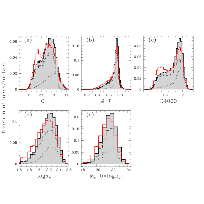
Figure 6: The fraction of the total mass of metals locked up in stars in the local Universe is shown as a function of various observable galaxy properties: (a) the concentration parameter, (b) the rest-frame $g-r$ colour, (c) the 4000Å-break index strength, (d) the stellar velocity dispersion and (e) the absolute $r$-band magnitude. The dotted line shows the contribution from high-S/N galaxies, while the dot-dashed line shows the contribution from low-S/N galaxies (obtained from high-S/N stacked spectra, see text for details). The continuous black line (grey-shaded histogram) shows the distribution obtained when both contributions are taken into account. The distribution of stellar mass as a function of the various properties is described by the red solid line in each panel. Note that the resolution in the distribution versus velocity dispersion and absolute magnitude is limited by the width of the bins in which low-S/N galaxies are grouped to obtain the co-added spectra (0.05 dex and 0.5 mag respectively).

Figure 7: Same as Fig. 6, but here the fraction of stellar mass and the fraction of metals in stars are shown as a function of the derived physical parameters: (a) $r$-band luminosity weighted age, (b) mass-weighted age (both ages are corrected to $z=0$ by the lookback time), (c) stellar mass and (d) stellar metallicity.

Table 6: For each parameter X, the percentiles of the distribution of stellar mass and of metals as a function of X are given. In the last column we indicate the mode of each distribution. The last row quotes the fraction of the total stellar mass in the local Universe contained in galaxies that contribute different fractions of the metal content.

Stellar mass distribution
Parameter	5%	10%	25%	50%	75%	90%	95%	mode
$\log\sigma_{V}$	$1.75_{-0.03}^{0.01}$	$1.83_{-0.03}^{+0.01}$	$1.98_{-0.03}^{+0.01}$	$2.12_{-0.03}^{+0.01}$	$2.24_{-0.02}^{+0.01}$	$2.34_{-0.01}^{+0.01}$	$2.38_{-0.01}^{+0.00{\dagger}}$	$2.20_{-0.05}^{+0.02}$
$M_{r}-5\times\log h_{70}$	$-23.17_{-0.03}^{+0.06}$	$-22.86_{-0.03}^{+0.04}$	$-22.33_{-0.03}^{+0.06}$	$-21.65_{-0.04}^{+0.09}$	$-20.90_{-0.04}^{+0.10}$	$-20.16_{-0.03}^{+0.08}$	$-19.69_{-0.03}^{+0.08}$	$-21.50_{-0.25}^{+0.25}$
$C$	$2.18_{-0.04}^{+0.01}$	$2.26_{-0.05}^{+0.01}$	$2.42_{-0.07}^{+0.02}$	$2.69_{-0.05}^{+0.02}$	$2.91_{-0.03}^{+0.02}$	$3.07_{-0.02}^{+0.01}$	$3.17_{-0.02}^{+0.01}$	$2.80_{-0.45}^{+0.05}$
$\rm D4000$	$1.24_{-0.01}^{+0.00{\dagger}}$	$1.30_{-0.02}^{+0.01}$	$1.45_{-0.04}^{+0.01}$	$1.73_{-0.05}^{+0.02}$	$1.89_{-0.02}^{+0.01}$	$1.97_{-0.01}^{+0.00{\dagger}}$	$2.01_{-0.01}^{+0.00{\dagger}}$	$1.92_{-0.02}^{+0.02}$
$g-r$	$0.44_{-0.02}^{+0.00{\dagger}}$	$0.51_{-0.03}^{+0.01}$	$0.62_{-0.03}^{+0.01}$	$0.71_{-0.01}^{+0.00{\dagger}}$	$0.74_{-0.00{\dagger}}^{+0.00{\dagger}}$	$0.77_{-0.00{\dagger}}^{+0.00{\dagger}}$	$0.79_{-0.00{\dagger}}^{+0.00{\dagger}}$	$0.74_{-0.01}^{+0.01}$
$\log(M_{\ast}/M_{\odot})$	$9.88_{-0.06}^{+0.06}$	$10.11_{-0.07}^{+0.06}$	$10.43_{-0.07}^{+0.06}$	$10.77_{-0.09}^{+0.06}$	$11.04_{-0.10}^{+0.06}$	$11.26_{-0.10}^{+0.06}$	$11.39_{-0.10}^{+0.07}$	$10.90_{-0.20}^{+0.10}$
$\log(Z_{\ast}/Z_{\odot})$	$-0.64_{-0.04}^{+0.06}$	$-0.47_{-0.05}^{+0.06}$	$-0.21_{-0.06}^{+0.05}$	$-0.03_{-0.07}^{+0.06}$	$0.09_{-0.07}^{+0.06}$	$0.17_{-0.07}^{+0.06}$	$0.20_{-0.04}^{+0.07}$	$0.10_{-0.10}^{+0.10}$
$\log(t_{r}/yr)$	$9.44_{-0.10}^{+0.08}$	$9.51_{-0.10}^{+0.09}$	$9.64_{-0.10}^{+0.08}$	$9.81_{-0.10}^{+0.06}$	$9.92_{-0.10}^{+0.07}$	$9.97_{-0.10}^{+0.09}$	$10.00_{-0.10}^{+0.10}$	$9.95_{-0.10}^{+0.05}$
$\log(t_{M}/yr)$	$9.57_{-0.09}^{+0.08}$	$9.64_{-0.09}^{+0.08}$	$9.74_{-0.09}^{+0.07}$	$9.86_{-0.09}^{+0.06}$	$9.94_{-0.09}^{+0.07}$	$9.99_{-0.09}^{+0.09}$	$10.02_{-0.09}^{+0.09}$	$9.95_{-0.05}^{+0.10}$
Stellar metallicity distribution
$\log\sigma_{V}$	$1.84_{-0.04}^{+0.01}$	$1.93_{-0.05}^{+0.01}$	$2.05_{-0.05}^{+0.01}$	$2.17_{-0.04}^{+0.01}$	$2.28_{-0.03}^{+0.01}$	$2.36_{-0.02}^{+0.01}$	$2.40_{-0.01}^{+0.01}$	$2.25_{-0.05}^{+0.02}$
$M_{r}-5\times\log h_{70}$	$-23.31_{-0.04}^{+0.11}$	$-22.98_{-0.05}^{+0.08}$	$-22.50_{-0.06}^{+0.12}$	$-21.91_{-0.06}^{+0.17}$	$-21.24_{-0.06}^{+0.15}$	$-20.61_{-0.05}^{+0.12}$	$-20.19_{-0.05}^{+0.13}$	$-22.00_{-0.25}^{+0.50}$
$C$	$2.21_{-0.07}^{+0.01}$	$2.31_{-0.08}^{+0.02}$	$2.53_{-0.11}^{+0.04}$	$2.77_{-0.08}^{+0.04}$	$2.96_{-0.06}^{+0.02}$	$3.10_{-0.04}^{+0.02}$	$3.20_{-0.04}^{+0.01}$	$2.95_{-0.25}^{+0.00{\dagger}}$
$\rm D4000$	$1.28_{-0.03}^{+0.01}$	$1.36_{-0.05}^{+0.02}$	$1.57_{-0.08}^{+0.03}$	$1.80_{-0.05}^{+0.02}$	$1.91_{-0.02}^{+0.01}$	$1.99_{-0.01}^{+0.00{\dagger}}$	$2.02_{-0.01}^{+0.00{\dagger}}$	$1.92_{-0.02}^{+0.02}$
$g-r$	$0.50_{-0.04}^{+0.01}$	$0.57_{-0.04}^{+0.01}$	$0.67_{-0.04}^{+0.01}$	$0.72_{-0.01}^{+0.00{\dagger}}$	$0.75_{-0.01}^{+0.00{\dagger}}$	$0.78_{-0.01}^{+0.00{\dagger}}$	$0.79_{-0.01}^{+0.00{\dagger}}$	$0.74_{-0.01}^{+0.01}$
$\log(M_{\ast}/M_{\odot})$	$10.12_{-0.06}^{+0.07}$	$10.30_{-0.07}^{+0.06}$	$10.59_{-0.09}^{+0.06}$	$10.86_{-0.15}^{+0.06}$	$11.10_{-0.13}^{+0.07}$	$11.31_{-0.13}^{+0.08}$	$11.44_{-0.13}^{+0.08}$	$10.90_{-0.20}^{+0.10}$
$\log(Z_{\ast}/Z_{\odot})$	$-0.34_{-0.05}^{+0.06}$	$-0.21_{-0.07}^{+0.05}$	$-0.07_{-0.07}^{+0.06}$	$0.05_{-0.07}^{+0.06}$	$0.14_{-0.07}^{+0.05}$	$0.20_{-0.04}^{+0.07}$	$0.25_{-0.05}^{+0.05}$	$0.10_{-0.10}^{+0.10}$
$\log(t_{r}/yr)$	$9.51_{-0.10}^{+0.08}$	$9.58_{-0.10}^{+0.08}$	$9.71_{-0.10}^{+0.07}$	$9.85_{-0.10}^{+0.06}$	$9.93_{-0.10}^{+0.08}$	$9.98_{-0.10}^{+0.10}$	$10.00_{-0.10}^{+0.10}$	$9.95_{-0.10}^{+0.10}$
$\log(t_{M}/yr)$	$9.63_{-0.09}^{+0.08}$	$9.68_{-0.09}^{+0.07}$	$9.78_{-0.09}^{+0.07}$	$9.89_{-0.09}^{+0.06}$	$9.96_{-0.09}^{+0.08}$	$10.00_{-0.09}^{+0.09}$	$10.03_{-0.09}^{+0.09}$	$9.95_{-0.05}^{+0.10}$
Fraction of the total stellar mass contributed
	0.106	0.178	0.351	0.592	0.806	0.925	0.962

†The estimated systematic uncertainty is smaller than 0.01, i.e. less than 20 percent of the bin size.

4.2 The characteristic age of the mass and metallicity distributions

We investigate further the distribution of metals and baryons as a function of stellar age. As shown in Fig. 7a,b both the stellar mass distribution and the metals distribution have a peak at a mean age of $\log(t/yr)=9.95$ (almost 9 Gyr). If we could translate this characteristic age into a redshift, it would correspond to a characteristic formation redshift of $z\sim 1.4$, which nicely falls in the redshift range over which the cosmic metal production rate and the cosmic star formation rate are expected to decline (e.g. Lilly et al., 1996; Madau et al., 1996; Madau et al., 1998; Glazebrook et al., 2004; Hopkins & Beacom, 2006, and references therein). This is of course only a naive interpretation, because we can only assign an average age (with a larger weight to younger stars) to individual galaxies and we cannot describe the real distribution of stellar ages within a galaxy. This is even more critical when the distribution in stellar metallicity is considered, as long as we assign a fixed metallicity to all stars in a galaxy, rather than following the chemical evolution along the star formation history. It is however interesting to notice that the result obtained from this ‘archaeological’ approach is close to what expected from ‘direct’ investigation of the cosmic star formation history.

Moreover, there is evidence that the timescale of star formation depends on the mass of the galaxy, with more massive galaxies having an early and shorter star formation, and less massive galaxies having a star formation more extended toward the present day. If so, the distribution of stellar ages in individual massive galaxies would be narrower than in less massive galaxies around the (mass- or light-weighted) average age, which would hence be more representative of the average formation redshift of the stars. It is thus useful to look at the distributions of baryon and metal densities in stars as a function of stellar age for galaxies with similar masses. These are shown in Fig. 8 (left- and right-hand panel respectively). The black continuous line shows the distribution of $\rho_{\ast}$ and $\rho_{Z}$ for the sample as a whole, while different colours and line styles correspond to different stellar mass bins (each distribution is normalized to the total $\rho_{\ast}$ and $\rho_{Z}$ in the corresponding mass bin). For reference, we indicate in the upper x-axis the redshift corresponding to the age on the lower x-axis (interpreted as lookback time from the present).

The distribution for the entire galaxy population is traced very well by the distribution of galaxies in the mass range between $3\times 10^{10}$ and $\rm 10^{11}M_{\odot}$, which alone contain 38 percent of the total stellar mass budget (these galaxies also provide the largest contribution to the star formation rate density and stellar mass density up to $z\sim 1$, as shown e.g. by Panter et al. (2006); Borch et al. (2006); Zheng et al. (2007)). This is true for both the stellar mass density and the metal density in stars. The contribution to the total baryon and metal budget in stars from galaxies with old stellar populations increases significantly from the lowest- to the highest-mass bin. This reflects the median relation between the galaxy mean age and stellar mass (see e.g. fig. 8 of paper I). Not only do the distributions in mass-weighted age shift gradually to younger ages as less massive galaxies are considered, but they also span larger ranges in age, a result of the increasing scatter in age at lower masses in the age-mass relationship.

Quantitatively, 25 percent of the total stellar mass and metal density of the most massive galaxies ($\rm>10^{11}M_{\odot}$) is contained in galaxies older than 9.5 Gyr, and half of it in galaxies older than 8.5 Gyr (corresponding to redshift greater than 1.2). As much as 75 percent of the stellar mass and metal density of low-mass galaxies (below $\rm 10^{10}M_{\odot}$) is distributed in galaxies with mass-weighted ages younger than $\sim$5.5 Gyr, and 50 percent in galaxies younger than $\sim$4.5 Gyr (corresponding to redshifts below $\sim$0.5). This trend is illustrated in Fig. 9. In each of the stellar mass bins defined in Fig. 8, we define two characteristic mass-weighted ages as the median of the distribution of stellar mass and the distribution of metals versus age. These characteristic ages are plotted as a function of stellar mass in Fig. 9. We also indicate the effect of individual sources of systematic uncertainties in each mass bin. The aperture bias and the scaled-solar abundance ratio of the models, in particular, affect to a larger extent more massive galaxies.

Despite the large uncertainties, it is clear from Fig. 9 that the characteristic ages of the stellar mass and metallicity distributions become progressively younger in less massive galaxies. This is in agreement (at least qualitatively) with the findings that the characteristic epoch at which the bulk of the stars (and metals) in present-day massive (mostly elliptical) galaxies formed is at redshift at least greater than 1 (e.g. Thomas et al., 2005, and references therein). Finally, it is worth noting that the characteristic age of the distribution of metals is never younger than the characteristic age of the distribution of mass. This is particularly true at masses below $\rm 10^{11}M_{\odot}$. This probably indicates that the correlation between age and stellar metallicity persists in individual stellar mass bins, with older galaxies being also more metal-rich. This correlation is weaker in higher-mass galaxies, because of the narrower ranges in both age and metallicity and because contrasted by the age-metallicity degeneracy (see e.g. figs. 11 and 12 of paper I).

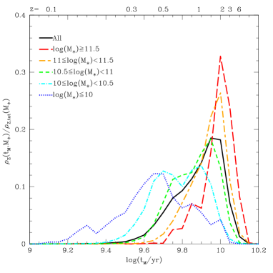
Figure 8: Differential distribution of stellar mass density (left panel) and mass density of metals in stars (right panels) as a function of mass-weighted age for the whole sample (continuous line). Different line styles distinguish the distribution for galaxies in different mass bins. Each distribution is normalized to the total $\rho_{\ast}$ and $\rho_{Z}$ in the corresponding mass bin. For reference the upper x-axis gives the redshift corresponding to a given mean age.

Figure 9: Mass-weighted age above which half of the total amount of mass (empty circles) and metals (filled circles) in stars are contained at the present epoch, as a function of stellar mass. Galaxies have been divided in the same five bins of stellar mass as in Fig. 8. Boxes and arrows quantify the ranges of the different sources of systematic uncertainties.

4.3 Comparison with the Millennium Simulation

The distribution functions of mass density of baryons and metals in stars provide important quantitative constraints at redshift zero against which models of galaxy formation and evolution in a cosmological context should be tested. We provide here a first comparison between our observational results and model predictions. We consider the results of the Millennium Run, the largest N-body simulation of structure formation carried out so far within the $\Lambda$CDM cosmological paradigm (Springel et al., 2005). We make use of the galaxy catalogues produced by semi-analytic galaxy formation algorithms run on the Millennium merger trees, as described in Croton et al. (2006) and De Lucia & Blaizot (2007), and select galaxies at $z=0$.

Before going into the detail of the distributions of metals and baryons in stars, we calculate the total $\rho_{\ast}$ and $\rho_{Z}$ predicted by the simulation. The total stellar mass density is $\rm 3.203\times 10^{8}~{}M_{\odot}~{}Mpc^{-3}$, in agreement with our determination as already mentioned in Section 3.3. The total mass density of metals in stars is instead $\rm 4.053\times 10^{6}~{}M_{\odot}~{}Mpc^{-3}$, lower than what observed (in particular it is $1.5\sigma$ lower than our result). This originates from the narrow metallicity distribution predicted by the models and the lower metallicity for massive galaxies, as we discuss below.

It is also of interest to mention the metal and baryon mass densities in other gaseous components, inside or outside galaxies, as predicted by the Millennium Simulation. The mass and metal densities in stars represent the 17.6 and 25.3 percent of the corresponding total values. Similar contributions (13.5 and 11.8 percent for the baryons and the metals, respectively) come from the gas ejected from galaxies into the surrounding intergalactic medium (see De Lucia et al., 2004). The cold gas inside galaxies provides only 6.6 percent and 9.8 percent to the total density of baryons and metals, respectively. The remaining 62.2 and 53.1 percent is contained in the hot gas component. The baryon fractions derived from the Millennium Simulation are in agreement with those predicted by the chemo-photometric models of Calura & Matteucci (2004). In both cases the fraction of baryons in stars is higher than what predicted by the simulations of Davé & Oppenheimer (2007) and than what we observe. The mass fraction of metals in stars predicted by the Millennium Simulation is instead about half of what quoted by Calura & Matteucci (2004) and Davé & Oppenheimer (2007).

We now discuss the contribution to the mass and metals in stars by different galaxies. After selecting galaxies at $z=0$ from the Millennium Catalogue, we construct the stellar mass-weighted distributions of baryons and metals in stars as functions of the galaxy stellar mass, mass-weighted age and stellar metallicity. Fig. 10 compares such distributions (gray-shaded histograms) with those derived from our SDSS measurements (solid lines).

Panels (a) and (d) of Fig. 10 illustrate the fraction of mass and metals as a function of stellar mass. The distributions predicted by the models display an offset in stellar mass with respect to the observationally derived distributions of $\sim$0.06 dex. We note that this offset is reduced when we use stellar masses based on Petrosian instead of model magnitudes (as shown by the dotted line). Comparison between the shaded and dotted histograms in panels (a) and (d) shows a good agreement between the observational results and the predictions from the simulations. It is clear, however, that the models predict too much mass in low-mass galaxies with respect to observations. This feature of the models has been already observed in the comparison with observational data of the $b_{J}$- and K-band luminosity function and the stellar mass function (see e.g. Croton et al., 2006; Bertone et al., 2007). Recently, Bertone et al. (2007) have presented a new implementation of a feedback scheme which incorporates a dynamical treatment of galactic winds powered by supernovae and by stellar winds, as alternative to empirically-motivated schemes of supernovae feedback, but without replacing AGN feedback. This treatment seems to alleviate the discrepancy in the galaxy stellar mass function, by reducing the abundance of low-mass galaxies and reaching a better agreement, in this respect, with observations.

Panels (b) and (e) show the fraction of baryons and metals in stars as a function of the galaxy mass-weighted age. While the predicted and observed distributions agree reasonably well at the oldest ages, there is clearly a deficit of young galaxies (with ages younger than $\log t=9.8$) in the simulations. This discrepancy could originate, at least in part, from the fact that, although we use mass-weighted ages for this comparison, the observationally derived mean ages are always extracted from fits to the galaxy spectra, and hence are always somehow weighted by light. This could thus give more weight to the youngest stellar populations in the galaxy. We note however that the tendency of the models to produce too old stellar populations with respect to those that we derive appears also in the relation between the light-weighted age and the stellar mass of elliptical galaxies (as seen in the comparison of fig. 6a of De Lucia et al. (2006) and fig. 17d of paper II), even though there is a good qualitative agreement.

Finally, panels (c) and (f) compares the predicted and observed distribution as a function of stellar metallicity. The disagreement between the observational result and model prediction is caused by the narrow stellar metallicity range spanned by the simulations. Moreover, while the observational trend of increasing metallicity with increasing mass is reproduced by the models, the predicted relation is too shallow with respect to observations, hardly reaching solar metallicity for the most massive galaxies. The galactic wind feedback scheme implemented by Bertone et al. (2007) seems to provide a better agreement with observations, causing a steepening of the mass-metallicity relation (due to the high efficiency of mass ejection in small haloes which suppresses star formation and hence the amount of metals that can be produced and locked up in stars) and predicting super-solar metallicities in massive galaxies.

As a general remark it is also interesting to notice the similarity between the distributions of mass and the corresponding distributions of metals in stars. While this is true also for the observationally derived distributions (as discussed in Section 4.1), it appears to a greater extent in the models. This originates from the narrower range in stellar metallicity and the shallower stellar metallicity/stellar mass relation with respect to observations.

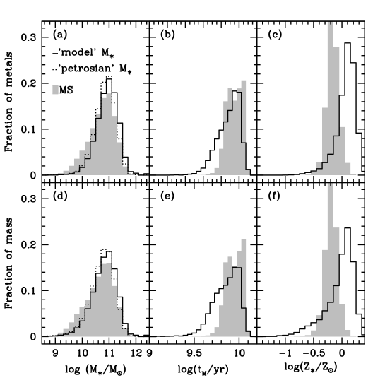
Figure 10: Comparison between predicted and observed distributions of stellar mass and metals. The fraction of metals in stars (upper panels) and the fraction of mass in stars (lower panels) are shown as functions of stellar mass (a,d), mass-weighted age (b,e), stellar metallicity (c,f). The shaded histograms show the distributions derived using the semi-analytic galaxy catalogue of the Millennium Simulation. The continuous line shows the results from our analysis on SDSS. The dotted histogram in panel (a) and (d) shows the results obtained when normalizing the mass-to-light ratio by the $z$-band Petrosian magnitude instead of model magnitude to derive stellar mass.

5 Summary and conclusions

In this work we have exploited recent estimates of physical parameters, such as stellar metallicity and stellar mass, for a comprehensive sample of more than $10^{5}$ nearby galaxies to derive the total mass density of metals and baryons locked up in stars in the local Universe, also expressed in terms of the present-day mass-weighted average stellar metallicity. Moreover, we have quantified the contribution to the total amount of metals by galaxies with different morphological and spectral properties, and compared the distribution of the stellar metallicity density with that of the stellar mass density.

The sample used is drawn from the SDSS DR2 and it includes galaxies spanning a wide range of star formation activity, from quiescent early-type to actively star-forming galaxies. The stellar metallicities, ages and stellar masses of these galaxies were previously derived (paper I) by comparing an optimally selected set of spectral absorption features to a comprehensive Monte Carlo library of model star formation histories (SFH), based on the high-resolution Bruzual & Charlot (2003) population synthesis code. We have shown in paper I that the uncertainties on the derived physical parameters directly depend on the mean spectral signal-to-noise ratio (S/N). Because of this, in previous work we have focused on galaxies with S/N greater than 20, biasing our sample towards more concentrated, higher surface brightness and higher velocity dispersion galaxies.

We need to include here also galaxies at lower S/N in order to derive a fair estimate of the total metallicity of stars at $z=0.1$. We do this by coadding (weighting by 1/$\rm V_{max}$) the spectra of low-S/N galaxies with similar $r$-band absolute magnitude, velocity dispersion and $\rm D4000$ until a minimum S/N requirement is satisfied. This allows us to derive estimates of the (1/$\rm V_{max}$-weighted average) stellar metallicity of low-S/N galaxies with an uncertainty not greater than 0.2 dex, i.e. comparable to the accuracy with which stellar metallicity is derived from individual high-S/N spectra. A similar improvement is obtained for light- and mass-weighted age and stellar mass, although these parameters are less affected than stellar metallicity by the quality of the spectrum.

We estimated the total mass density of baryons and of metals locked up in stars in the local Universe, by combining the contribution of the individual high-S/N galaxies and the low-S/N galaxies, as derived from the coadded spectra. We find, respectively, $\rho_{\ast}=3.413\pm 0.005^{+0.569}_{-0.554}\times 10^{8}~{}h_{70}~{}\rm M_{\odot}~{}Mpc^{-3}$ and $\rho_{Z}=7.099\pm 0.019^{+2.184}_{-1.943}\times 10^{6}~{}h_{70}~{}\rm M_{\odot}~{}Mpc^{-3}$. This is in broad agreement with other measures from the literature, which however span a relatively large range. The measure of the metal mass density is perhaps more significant in discriminating different model predictions or approaches. We find a reasonably good agreement with results of chemical evolution models, such as those of Pei et al. (1999) or Calura & Matteucci (2004). Hydrodynamic simulations seem to predict values of $\rho_{Z}$ at the lower end of the observational constraints. The total amount of metals locked up in stars is sensitive to the feedback efficiency, which regulates the amount of gas and metals expelled from galaxies. Integration of cosmic star formation histories, on the other hand, in general overpredicts the total amount of metals in stars. This is probably due to poor knowledge of dust corrections at high redshift and uncertainties on the average metal yield to convert star formation rate into metal production rate.

By combining the densities of mass and metals in stars we can estimate the average stellar metallicity today to be consistent with solar (Equation 6). This is not surprising, given that the stellar mass budget is dominated, at least in the local Universe, by galaxies just above the transition mass (approximately $L^{\ast}$ galaxies), which have typically solar metallicity. This value is in agreement with the prediction of the chemo-photometric models of Calura & Matteucci (2004) and the result of Edmunds & Phillipps (1997).

The good statistics available from the SDSS allows us to provide an analysis of the distribution of the stellar metallicity density as a function of global galaxy properties (such as velocity dispersion, luminosity and stellar mass), as a function of morphology (as approximated by the concentration parameter), and as a function of spectral and physical properties of the stellar populations (such as colour and 4000Å-break strength, stellar age and metallicity). We have compared such distributions with the corresponding distributions of stellar mass density. Our study has shown that the stellar metallicity and the stellar mass distributions do not differ significantly, in particular at the high-mass end. In other words, the galaxies that contribute most of the total amount of metals in stars have properties similar to those containing the bulk of the total mass in stars.

The typical galaxy in the present-day Universe where baryons and metals reside has a concentration parameter of 2.7 (indicating a disc and a significant bulge component), a $\hbox{$\rm D4000$}=1.7$, corresponding to a fairly old stellar age of $\sim$6 Gyr, and a stellar mass of $6\times 10^{10}M_{\odot}$. Note that the characteristic mass found here is above the stellar mass of $3\times 10^{10}M_{\odot}$ at which the transition from low-mass, metal-poor, disc-dominated galaxies to high-mass, metal-rich, bulge-dominated galaxies occurs. Galaxies with masses greater than $3\times 10^{10}M_{\odot}$, where the mass-metallicity relation starts to flatten (Tremonti et al., 2004; Gallazzi et al., 2005), contain more than 80 percent of the total amount of mass and metals in stars.

The stellar metallicity and stellar mass distributions differ most significantly with respect to concentration and stellar age (as indicated also by the colour and $\rm D4000$), in the sense that the relative contributions to the total stellar mass and to the total metallicity are reversed in late-type galaxies, compared to early-type galaxies (morphologically or photometrically classified as such). Separating galaxies on the basis of their concentration parameter, we find that bulge-dominated and disc-dominated galaxies provide the same fraction of the total mass in stars (30 or 50 percent depending on the cut in $C$ adopted). On the contrary, the contribution of disc-dominated galaxies to the mass density of metals is lower than that of bulge-dominated galaxies (with the same cuts in concentration). For example, defining early-type galaxies as those having $C\geq 2.8$ and late-types those having $C\leq 2.4$, the two classes of galaxies both contribute 30 percent to the stellar mass budget, but 40 and less than 25 percent respectively to the total metal budget in stars.

Similar considerations hold for the distributions as functions of colour or $\rm D4000$. We find that at least 50 up to 75 percent of the stellar mass (and of the metals) is locked into red-sequence galaxies (depending on the assumed colour cut). These fractions are in good agreement with previous results from e.g. Bell et al. (2003) and Baldry et al. (2004). We show that these observational distributions are physically translated into the corresponding distributions in age. More than 50 percent of the mass and the metals locked up in stars reside in galaxies with ages older than 6.3 Gyr.

It would be tempting to translate the characteristic age of the stellar populations contributing most of the metals and of the mass into a characteristic redshift of formation. Unfortunately, this cannot be done straightforwardly because our stellar ages are averages over all the stellar populations in a galaxy, weighted by mass or by light. Thus they are very sensitive to the galaxy SFH and, on average, closer to the last significant episode of star formation. Given the different timescales of star formation expected in galaxies with different mass, it is reasonable to look at the distributions of mass and metals against (mass-weighted) age for different stellar mass bins. This shows that most of the mass and metals come from galaxies older than a characteristic age which becomes progressively younger from massive to less massive galaxies. Considering only massive galaxies ($\rm>10^{11}M_{\odot}$) at least 50 percent of the mass and metals is in systems older than 8.5 Gyr, which would correspond to a redshift $z>1.2$. This redshift is compatible with the redshift range $1<z<2$ at which the cosmic star formation rate density starts to decline (e.g. Hopkins & Beacom, 2006). This is consistent with the evidence that the bulk of star formation in massive galaxies has occurred at high redshifts, while low-mass galaxies are still in a phase of active star formation (e.g. Brinchmann & Ellis, 2000; Juneau et al., 2005; Bundy et al., 2005), although galaxies appear to experience the same rate of decline in their global star formation from $z\sim$1 to the present independently of mass (Zheng et al., 2007).

Comparison of the observed distributions of $\rho_{Z}$ and $\rho_{\ast}$ with those predicted by the Millennium Simulation shows a good agreement in the distributions against stellar mass. However, an excess at low stellar masses (roughly below $\rm 3\times 10^{10}M_{\odot}$) is visible, which has been already pointed out in the luminosity or stellar mass functions (see e.g. Croton et al., 2006). The agreement between our observations and the models becomes worse when mass-weighted age and stellar metallicity are considered. Although successful in reproducing the general trend of increasing both age and metallicity with mass (e.g. De Lucia et al., 2006), the models predict narrower ranges in these physical parameters than observed.

Our study provides a new determination of the total amount of metals locked up in stars today and allows us for the first time to derive a quantitative and accurate description of the properties of the galaxies hosting different fractions of the metals and of the stellar mass in the local Universe. Such distributions represent important constraints on models of the cosmic star formation and chemical enrichment histories. The detailed knowledge of the distribution of metals, coupled to the stellar mass distribution, will allow a more direct comparison with predictions from semianalytic models of galaxy formation and evolution. Ongoing large redshift surveys, like VVDS (Le Fèvre et al., 2004), GOODS (Dickinson et al., 2003a; Vanzella et al., 2005), DEEP2 (Davis et al., 2003; Madgwick et al., 2003), zCOSMOS (Lilly et al., 2006), will make it possible to extend this kind of studies to redshifts as high as $z\sim 1$ and thus, not only to build a more consistent picture of the cosmic star formation history, but also to understand which are the galaxies that most strongly contributed to its evolution since $z=1$.

References

- Abazajian et al. (2004) Abazajian K., et al. 2004, AJ, 128, 502
- Abraham et al. (2004) Abraham R. G., et al 2004, AJ, 127, 2455
- Allende Prieto et al. (2001) Allende Prieto C., Lambert D. L., Asplund M., 2001, ApJ, 556, L63
- Asplund et al. (2005) Asplund M., Grevesse N., Sauval A. J., 2005, in Cosmic Abundances as Records of Stellar Evolution and Nucleosynthesis. Edited by Barnes and Bash.Astronomical Society of the Pacific Conference Series, Volume 336, pp. 25+ (2005).
- Asplund (2005) Asplund M., 2005, ARA&A, 43, 481
- Baldry et al. (2002) Baldry I. K., et al 2002, ApJ, 569, 582
- Baldry et al. (2004) Baldry I. K., Glazebrook K., Brinkmann J., Ivezić Ž., Lupton R. H., Nichol R. C., Szalay A. S., 2004, ApJ, 600, 681
- Baugh et al. (1998) Baugh C. M., Cole S., Frenk C. S., Lacey C. G., 1998, ApJ, 498, 504
- Bell & de Jong (2001) Bell, E. F. and de Jong, R. S., 2001, ApJ, 550, 212
- Bell et al. (2003) Bell E. F., McIntosh D. H., Katz N., Weinberg M. D., 2003, ApJS, 149, 289
- (11) Bell E. F., Zheng X. Z., Papovich C., Borch A., Wolf C., Meisenheimer K., 2007,ApJ,663,834
- Bernardi et al. (2003b) Bernardi M., et al. 2003, AJ, 125, 1849
- Bertone et al. (2007) Bertone S., De Lucia G., Thomas P. A., 2007, MNRAS, 379, 1143
- Blanton et al. (2003) Blanton M. R., et al. 2003, ApJ, 592, 819
- Borch et al. (2006) Borch A., Meisenheimer K., Bell E. F., Rix H.-W., Wolf C., Dye S., Kleinheinrich M., Kovacs Z., Wisotzki L., 2006, A&A, 453, 869
- Bouché et al. (2005) Bouché N., Lehnert M. D., Péroux C., 2005, MNRAS, 364, 319
- Bouché et al. (2007) Bouché N., Lehnert M. D., Aguirre A., Peroux C., Bergeron J., 2007, MNRAS, 378, 525
- (18) Bresolin, F. and Garnett, D. R. and Kennicutt, Jr., R. C., 2004, ApJ, 615, 228
- Brinchmann et al. (2004) Brinchmann J., Charlot S., White S. D. M., Tremonti C., Kauffmann G., Heckman T., Brinkmann J., 2004, MNRAS, 351, 1151
- Brinchmann & Ellis (2000) Brinchmann J., Ellis R. S., 2000, ApJ, 536, L77
- Bruzual & Charlot (2003) Bruzual G., Charlot S., 2003, MNRAS, 344, 1000
- Bundy et al. (2005) Bundy K., Ellis R. S., Conselice C. J., 2005, ApJ, 625, 621
- Calura & Matteucci (2004) Calura F., Matteucci F., 2004, MNRAS, 350, 351
- Chabrier (2003) Chabrier G., 2003, PASP, 115, 763
- Cid Fernandes et al. (2007) Cid Fernandes R., Asari N. V., Sodré L., Stasińska G., Mateus A., Torres-Papaqui J. P., Schoenell W., 2007, MNRAS, 375, L16
- Cole et al. (2001) Cole S., et al. 2001, MNRAS, 326, 255
- Cole et al. (2000) Cole S., Lacey C. G., Baugh C. M., Frenk C. S., 2000, MNRAS, 319, 168
- Colless et al. (2001) Colless M., et al 2001, MNRAS, 328, 1039
- Connolly et al. (1997) Connolly A. J., Szalay A. S., Dickinson M., Subbarao M. U., Brunner R. J., 1997, ApJ, 486, L11+
- Conti et al. (2003) Conti A., Connolly A. J., Hopkins A. M., Budavári T., Szalay A. S., Csabai I., Schmidt S. J., Adams C., Petrovic N., 2003, AJ, 126, 2330
- Cowie et al. (1999) Cowie L. L., Songaila A., Barger A. J., 1999, AJ, 118, 603
- Croton et al. (2006) Croton D. J., et al 2006, MNRAS, 365, 11
- Davé & Oppenheimer (2007) Davé R., Oppenheimer B. D., 2007, MNRAS, 374, 427
- Davis et al. (2003) Davis M. et al. 2003, in Discoveries and Research Prospects from 6- to 10-Meter-Class Telescopes II. Edited by Guhathakurta, Puragra. Proceedings of the SPIE, Volume 4834, pp. 161-172. Science Objectives and Early Results of the DEEP2 Redshift Survey.
- De Lucia & Blaizot (2007) De Lucia G., Blaizot J., 2007, MNRAS, 375, 2
- De Lucia et al. (2006) De Lucia G., Springel V., White S. D. M., Croton D., Kauffmann G., 2006, MNRAS, 366, 499
- De Lucia et al. (2004) De Lucia G., Kauffmann G., White S. D. M., 2004, MNRAS, 349, 1101
- Dickinson et al. (2003a) Dickinson M., Giavalisco M., The Goods Team 2003a, in The Mass of Galaxies at Low and High Redshift. Edited by Bender R., Renzini A., p.324
- Dickinson et al. (2003) Dickinson M., Papovich C., Ferguson H. C., Budavári T., 2003b, ApJ, 587, 25
- Driver et al. (2007a) Driver S. P., Allen P. D., Liske J., Graham A. W., 2007a, ApJ, 657L, 85
- Driver et al. (2007b) Driver S. P., Popescu C. C., Tuffs R. J., Liske J., Graham A. W., Allen P. D., De Propris R., 2007b, MNRAS, 379, 1022
- Dunne et al. (2003) Dunne L., Eales S. A., Edmunds M. G., 2003, MNRAS, 341, 589
- Edmunds & Phillipps (1997) Edmunds M. G., Phillipps S., 1997, MNRAS, 292, 733
- Ellison et al. (2005) Ellison S. L., Kewley L. J., Mallén-Ornelas G., 2005, MNRAS, 357, 354
- Erb et al. (2006) Erb D. K., Shapley A. E., Pettini M., Steidel C. C., Reddy N. A., Adelberger K. L., 2006, ApJ, 644, 813
- Ferrara et al. (2005) Ferrara A., Scannapieco E., Bergeron J., 2005, ApJ, 634, L37
- Fukugita et al. (1998) Fukugita M., Hogan C. J., Peebles P. J. E., 1998, ApJ, 503, 518
- Fukugita & Peebles (2004) Fukugita M., Peebles P. J. E., 2004, ApJ, 616, 643
- Gallazzi et al. (2006) Gallazzi A., Charlot S., Brinchmann J., White S. D. M., 2006, MNRAS, 370, 1106
- Gallazzi et al. (2005) Gallazzi A., Charlot S., Brinchmann J., White S. D. M., Tremonti C. A., 2005, MNRAS, 362, 41
- Glazebrook et al. (2003) Glazebrook K., et al. 2003, ApJ, 587, 55
- Glazebrook et al. (2004) Glazebrook K., Tober J., Thomson S., Bland-Hawthorn J., Abraham R., 2004, AJ, 128, 2652
- Heavens et al. (2004) Heavens A., Panter B., Jimenez R., Dunlop J., 2004, Nature, 428, 625
- Heavens et al. (2000) Heavens A. F., Jimenez R., Lahav O., 2000, MNRAS, 317, 965
- Henry & Worthey (1999) Henry R. B. C., Worthey G., 1999, PASP, 111, 919
- Hernquist & Springel (2003) Hernquist L., Springel V., 2003, MNRAS, 341, 1253
- Hopkins & Beacom (2006) Hopkins A. M., Beacom J. F., 2006, ApJ, 651, 142
- Ivison et al. (2002) Ivison R. J., et al 2002, MNRAS, 337, 1
- Jimenez et al. (2005) Jimenez R., Panter B., Heavens A. F., Verde L., 2005, MNRAS, 356, 495
- Juneau et al. (2005) Juneau S., Glazebrook K., Crampton D., McCarthy P. J., Savaglio S., Abraham R., Carlberg R. G., Chen H.-W., Le Borgne D., Marzke R. O., Roth K., Jørgensen I., Hook I., Murowinski R., 2005, ApJ, 619, L135
- Kauffmann et al. (2003) Kauffmann G. et al. 2003, MNRAS, 341, 33
- Kobayashi et al. (2006) Kobayashi C., Springel V., White S. D. M., 2006, ApJ, 653, 1145
- Kobulnicky & Kewley (2004) Kobulnicky H. A., Kewley L. J., 2004, ApJ, 617, 240
- Kobulnicky & Zaritsky (1999) Kobulnicky H. A., Zaritsky D., 1999, ApJ, 511, 118
- Kochanek et al. (2001) Kochanek C. S., Pahre M. A., Falco E. E., Huchra J. P., Mader J., Jarrett T. H., Chester T., Cutri R., Schneider S. E., 2001, ApJ, 560, 566
- Korn et al. (2005) Korn A. J., Maraston C., Thomas D., 2005, A&A, 438, 685
- Lanzetta et al. (1995) Lanzetta K. M., Wolfe A. M., Turnshek D. A., 1995, ApJ, 440, 435
- Le Fèvre et al. (2004) Le Fèvre O., et al 2004, A&A, 428, 1043
- Lilly et al. (1996) Lilly S. J., Le Fevre O., Hammer F., Crampton D., 1996, ApJ, 460, L1+
- Lilly et al. (2003) Lilly S. J., Carollo C. M., Stockton A. N., 2003, ApJ, 597, 730
- Lilly et al. (2006) Lilly S. J. et al. ,2007, ApJS, 172, 70
- MacArthur et al. (2004) MacArthur L. A., Courteau S., Bell E., Holtzman J. A., 2004, ApJS, 152, 175
- Madau et al. (1996) Madau P., Ferguson H. C., Dickinson M. E., Giavalisco M., Steidel C. C., Fruchter A., 1996, MNRAS, 283, 1388
- Madau et al. (1998) Madau P., Pozzetti L., Dickinson M., 1998, ApJ, 498, 106
- Madgwick et al. (2003) Madgwick D. S., et al 2003, ApJ, 599, 997
- Mehlert et al. (2003) Mehlert D., Thomas D., Saglia R. P., Bender R., Wegner G., 2003, A&A, 407, 423
- Monaco et al. (2007) Monaco P., Fontanot F., Taffoni G., 2007, MNRAS, 375, 1189
- Nagamine et al. (2006) Nagamine K., Ostriker J. P., Fukugita M., Cen R., 2006, ApJ, 653, 881
- (79) Ocvirk, P. and Pichon, C. and Lançon, A. and Thiébaut, E, 2006, MNRAS, 365, 74
- Pagel (2002) Pagel B. E. J., 2002, in ASP Conf. Ser. 253: Chemical Enrichment of Intracluster and Intergalactic Medium Metals in the Universe and Diffuse Background Radiation. (I). pp 489–+
- Panter et al. (2006) Panter B., Jimenez R., Heavens A. F., Charlot S., 2007, MNRAS, 378, 1550
- Pei & Fall (1995) Pei Y. C., Fall S. M., 1995, ApJ, 454, 69
- Pei et al. (1999) Pei Y. C., Fall S. M., Hauser M. G., 1999, ApJ, 522, 604
- Péroux et al. (2003) Péroux C., Dessauges-Zavadsky M., D’Odorico S., Kim T.-S., McMahon R. G., 2003, MNRAS, 345, 480
- Péroux et al. (2005) Péroux C., Dessauges-Zavadsky M., D’Odorico S., Sun Kim T., McMahon R. G., 2005, MNRAS, 363, 479
- Péroux et al. (2006) Péroux C., Meiring J. D., Kulkarni V. P., Ferlet R., Khare P., Lauroesch J. T., Vladilo G., York D. G., 2006, MNRAS, 372, 369
- Pettini (2006) Pettini M., 2006, in The Fabulous Destiny of Galaxies: Bridging Past and Present. Proc. of the Vth Marseille International Cosmology conference, Marseille. Edited by V. LeBrun, A. Mazure, S. Arnouts and D. Burgarella, p.319
- Pettini et al. (2001) Pettini M., Shapley A. E., Steidel C. C., Cuby J.-G., Dickinson M., Moorwood A. F. M., Adelberger K. L., Giavalisco M., 2001, ApJ, 554, 981
- Pettini et al. (1994) Pettini M., Smith L. J., Hunstead R. W., King D. L., 1994, ApJ, 426, 79
- Pettini et al. (1997) Pettini M., Smith L. J., King D. L., Hunstead R. W., 1997, ApJ, 486, 665
- Prochaska et al. (2007) Prochaska L. C., Rose J. A., Caldwell N., Castilho B. V., Concannon K., Harding P., Morrison H., Schiavon R. P., 2007, AJ, 134, 321
- Rudnick et al. (2003) Rudnick G., et al. 2003, ApJ, 599, 847
- Rudnick et al. (2006) Rudnick G., et al. 2006, ApJ, 650, 624
- Salpeter (1955) Salpeter E. E., 1955, ApJ, 121, 161
- Salucci & Persic (1999) Salucci P., Persic M., 1999, MNRAS, 309, 923
- (96) Shankar F., Lapi A., Salucci P., De Zotti G., Danese L., 2006, ApJ, 643, 14
- Schlegel et al. (1998) Schlegel D. J., Finkbeiner D. P., Davis M., 1998, ApJ, 500, 525
- Shapley et al. (2004) Shapley A. E., Erb D. K., Pettini M., Steidel C. C., Adelberger K. L., 2004, ApJ, 612, 108
- Springel et al. (2005) Springel V., et al. 2005, Nature, 435, 629
- Steidel et al. (1999) Steidel C. C., Adelberger K. L., Giavalisco M., Dickinson M., Pettini M., 1999, ApJ, 519, 1
- Steidel et al. (2004) Steidel C. C., Shapley A. E., Pettini M., Adelberger K. L., Erb D. K., Reddy N. A., Hunt M. P., 2004, ApJ, 604, 534
- Strateva et al. (2001) Strateva I., et al. 2001, AJ, 122, 1861
- Thomas et al. (2005) Thomas D., Maraston C., Bender R., de Oliveira C. M., 2005, ApJ, 621, 673
- Thomas et al. (2004) Thomas D., Maraston C., Korn A., 2004, MNRAS, 351, L19
- Tojeiro et al. (2007) Tojeiro, R. and Heavens, A. F. and Jimenez, R. and Panter, B., 2007, MNRAS, 381, 1252
- Tremonti et al. (2004) Tremonti C. A., et al. 2004, ApJ, 613, 898
- Vanzella et al. (2005) Vanzella E., et al 2005, A&A, 434, 53
- York et al. (2000) York D. G., et al. 2000, AJ, 120, 1579
- Zheng et al. (2006) Zheng X. Z., Bell E. F., Rix H.-W., Papovich C., Le Floc’h E., Rieke G. H., Pérez-González P. G., 2006, ApJ, 640, 784
- Zheng et al. (2007) Zheng X. Z., Bell E. F., Papovich C., Wolf C., Meisenheimer K., Rix H.-W., Rieke G. H., Somerville R., 2007, ApJ, 661, L41