INSTITUT NATIONAL DE RECHERCHE EN INFORMATIQUE ET EN AUTOMATIQUE

Quasi-stationary distributions
as centrality measures of reducible graphs
Konstantin Avrachenkov — Vivek Borkar — Danil Nemirovsky N° 6263
August 2007

Abstract: Random walk can be used as a centrality measure of a directed graph. However, if the graph is reducible the random walk will be absorbed in some subset of nodes and will never visit the rest of the graph. In Google PageRank the problem was solved by introduction of uniform random jumps with some probability. Up to the present, there is no clear criterion for the choice this parameter. We propose to use parameter-free centrality measure which is based on the notion of quasi-stationary distribution. Specifically we suggest four quasi-stationary based centrality measures, analyze them and conclude that they produce approximately the same ranking. The new centrality measures can be applied in spam detection to detect “link farms” and in image search to find photo albums.

Key-words: centrality measure, directed graph, quasi-stationary distribution, PageRank, Web graph, link farm

Résumé : Une marche au hasard peut être utilisée comme mesure de centralité d’un graphe orienté. Cependant, si le graphe est réductible la marche au hasard sera absorbée dans un quelque sous-ensemble de noeuds et ne visitera jamais le reste du graphe. Dans Google PageRank, le problème a été résolu par l’introduction des sauts aléatoires uniformes avec une certaine probabilité. Jusqu’à présent, il n’y a aucun critère clair pour le choix de ce paramètre. Nous proposons d’utiliser la mesure de centralité sans paramètre qui est basée sur la notion de la distribution quasi-stationnaire. Nous analysons les quatre mesures et concluons qu’elles produisent presque le même classement de noeuds. Les nouvelles mesures de centralité peuvent être appliquées dans le context de la détection de spam pour détecter les “link farms” et dans le context de la recherche d’image pour trouver des albums photo.

Mots-clés : mesure de centralité, marche au hasard, graphe orienté, distribution quasi-stationnaire, PageRank, graphe du Web, link farm

1 Introduction

Random walk can be used as a centrality measure of a directed graph. An example of random walk based centrality measures is PageRank [21] used by search engine Google. PageRank is used by Google to sort the relevant answers to user’s query. We shall follow the formal definition of PageRank from [18]. Denote by $n$ the total number of pages on the Web and define the $n\times n$ hyperlink matrix $P$ such that

$$p_{ij}=\left\{\begin{array}[]{ll}1/d_{i},&\mbox{if page $i$ links to $j$},\\ 1/n,&\mbox{if page $i$ is dangling},\\ 0,&\mbox{otherwise},\end{array}\right.$$ (1)

for $i,j=1,...,n$, where $d_{i}$ is the number of outgoing links from page $i$. A page with no outgoing links is called dangling. We note that according to (1) there exist artificial links to all pages from a dangling node. In order to make the hyperlink graph connected, it is assumed that at each step, with some probability $c$, a random surfer goes to an arbitrary Web page sampled from the uniform distribution. Thus, the PageRank is defined as a stationary distribution of a Markov chain whose state space is the set of all Web pages, and the transition matrix is

$$G=cP+(1-c)(1/n)E,$$

where $E$ is a matrix whose all entries are equal to one, and $c\in(0,1)$ is a probability of following a hyperlink. The constant $c$ is often referred to as a damping factor. The Google matrix $G$ is stochastic, aperiodic, and irreducible, so the PageRank vector $\pi$ is the unique solution of the system

$$\pi G=\pi,\quad\pi{\bf 1}=1,$$

where ${\bf 1}$ is a column vector of ones.

Even though in a number of recent works, see e.g., [5, 6, 8], the choice of the damping factor $c$ has been discussed, there is still no clear criterion for the choice of its value. The goal of the present work is to explore parameter-free centrality measures.

In [5, 7, 15] the authors have studied the graph structure of the Web. In particular, in [7, 15] it was shown that the Web Graph can be divided into three principle components: the Giant Strongly Connected Component, to which we simply refer as SCC component, the IN component and the OUT component. The SCC component is the largest strongly connected component in the Web Graph. In fact, it is larger than the second largest strongly connected component by several orders of magnitude. Following hyperlinks one can come from the IN component to the SCC component but it is not possible to return back. Then, from the SCC component one can come to the OUT component and it is not possible to return to SCC from the OUT component. In [7, 15] the analysis of the structure of the Web was made assuming that dangling nodes have no outgoing links. However, according to (1) there is a probability to jump from a dangling node to an arbitrary node. This can be viewed as a link between the nodes and we call such a link the artificial link. As was shown in [5], these artificial links significantly change the graph structure of the Web. In particular, the artificial links of dangling nodes in the OUT component connect some parts of the OUT component with IN and SCC components. Thus, the size of the Giant Strongly Connected Component increases further. If the artificial links from dangling nodes are taken into account, it is shown in [5] that the Web Graph can be divided in two disjoint components: Extended Strongly Connected Component (ESCC) and Pure OUT (POUT) component. The POUT component is small in size but if the damping factor $c$ is chosen equal to one, the random walk absorbs with probability one into POUT. We note that nearly all important pages are in ESCC. We also note that even if the damping factor is chosen close to one, the random walk can spend a significant amount of time in ESCC before the absorption. Therefore, for ranking Web pages from ESCC we suggest to use the quasi-stationary distributions [9, 22].

It turns out that there are several versions of quasi-stationary distribution. Here we study four versions of the quasi-stationary distribution. Our main conclusion is that the rankings provided by them are very similar. Therefore, one can chose a version of stationary distribution which is easier for computation.

The paper is organized as follows: In the next Section 2 we discuss different notions of quasi-stationarity, the relation among them, and the relation between the quasi-stationary distribution and PageRank. Then, in Section 3 we present the results of numerical experiments on Web Graph which confirm our theoretical findings and suggest the application of quasi-stationarity based centrality measures to link spam detection and image search. Some technical results we place in the Appendix.

2 Quasi-stationary distributions as centrality measures

As noted in [5], by renumbering the nodes the transition matrix $P$ can be transformed to the following form

$$P=\left[\begin{array}[]{cc}Q&0\\ R&T\end{array}\right],$$

where the block $T$ corresponds to the ESCC, the block $Q$ corresponds to the part of the OUT component without dangling nodes and their predecessors, and the block $R$ corresponds to the transitions from ESCC to the nodes in block $Q$. We refer to the set of nodes in the block $Q$ as POUT component.

The POUT component is small in size but if the damping factor $c$ is chosen equal to one, the random walk absorbs with probability one into POUT. We are mostly interested in the nodes in the ESCC component. Denote by $\pi_{Q}$ a part of the PageRank vector corresponding to the POUT component and denote by $\pi_{T}$ a part of the PageRank vector corresponding to the ESCC component. Using the following formula [20]

$$\pi(c)=\frac{1-c}{n}{\bf 1}^{T}[I-cP]^{-1},$$

we conclude that

$$\pi_{T}(c)=\frac{1-c}{n}{\bf 1}^{T}[I-cT]^{-1},$$

where ${\bf 1}$ is a vector of ones of appropriate dimension.

Let us define

$$\hat{\pi}_{T}(c)=\frac{\pi_{T}(c)}{||\pi_{T}(c)||_{1}}.$$

Since the matrix $T$ is substochastic, we have the next result.

Proposition 1

The following limit exists

$$\hat{\pi}_{T}(1)=\lim_{c\to 1}\frac{\pi_{T}(c)}{||\pi_{T}(c)||_{1}}=\frac{{\bf 1}^{T}[I-T]^{-1}}{{\bf 1}^{T}[I-T]^{-1}{\bf 1}},$$

and the ranking of pages in ESCC provided by the PageRank vector converges to the ranking provided by $\hat{\pi}_{T}(1)$ as the damping factor goes to one. Moreover, these two rankings coincide for all values of $c$ above some value $c^{*}$.

Next we denote $\hat{\pi}_{T}(1)$ simply by $\hat{\pi}_{T}$. Following [9, 12] we shall call the vector $\hat{\pi}_{T}$ pseudo-stationary distribution. The $i^{\textrm{th}}$ component of $\hat{\pi}_{T}$ can be interpreted as a fraction of time the random walk (with $c=1$) spends in node $i$ prior to absorption. We recall that the random walk as defined in Introduction starts from the uniform distribution. If the random walk were initiated from another distribution, the pseudo-stationary distribution would change.

Denote by $\bar{T}$ the hyperlink matrix associated with ESCC when the links leading outside of ESCC are neglected. Clearly, we have

$$\bar{T}_{ij}=\frac{T_{ij}}{[T{\bf 1}]_{i}},$$

where $[T{\bf 1}]_{i}$ denotes the $i^{\textrm{th}}$ component of vector $T{\bf 1}$. In other words, $[T{\bf 1}]_{i}$ is the sum of elements in row $i$ of matrix $T$. The $\bar{T}_{ij}$ entry of the matrix $\bar{T}$ can be considered as a conditional probability to jump from the node $i$ to the node $j$ under the condition that random walk does not leave ESCC at the jump. Let $\bar{\pi}_{T}$ be a stationary distribution of $\bar{T}$.

Let us now consider the substochastic matrix $T$ as a perturbation of stochastic matrix $\bar{T}$. We introduce the perturbation term

$$\varepsilon D=\bar{T}-T,$$

where the parameter $\varepsilon$ is the perturbation parameter, which is typically small. The following result holds.

Proposition 2

The vector $\hat{\pi}_{T}$ is close to $\bar{\pi}_{T}$. Namely,

$$\hat{\pi}_{T}=\bar{\pi}_{T}-\bar{\pi}_{T}\frac{1}{n_{T}}(\bar{\pi}_{T}\varepsilon D{\bf 1}){\bf 1}^{T}X_{0}{\bf 1}+{\bf 1}^{T}X_{0}\frac{1}{n_{T}}(\bar{\pi}_{T}\varepsilon D{\bf 1})+o(\varepsilon),$$ (2)

where $n_{T}$ is the number of nodes in ESCC and $X_{0}$ is given in Lemma 1 from the Appendix.

Proof: We substitute $T=\bar{T}-\varepsilon D$ into $[I-T]^{-1}$ and use Lemma 1, to get

$$[I-T]^{-1}=\frac{1}{\bar{\pi}\varepsilon D{\bf 1}}{\bf 1}\bar{\pi}+X_{0}+O(\varepsilon).$$

Using the above expression, we can write

$$\hat{\pi}_{T}=\frac{{\bf 1}^{T}[I-T]^{-1}}{{\bf 1}^{T}[I-T]^{-1}{\bf 1}}=\frac{\frac{1}{\bar{\pi}_{T}\varepsilon D{\bf 1}}n_{T}\bar{\pi}_{T}+{\bf 1}^{T}X_{0}+O(\varepsilon)}{\frac{1}{\bar{\pi}_{T}\varepsilon D{\bf 1}}n_{T}+{\bf 1}^{T}X_{0}{\bf 1}+O(\varepsilon)}=\frac{\bar{\pi}_{T}+\frac{1}{n_{T}}(\bar{\pi}_{T}\varepsilon D{\bf 1}){\bf 1}^{T}X_{0}+o(\varepsilon)}{1+\frac{1}{n_{T}}(\bar{\pi}_{T}\varepsilon D{\bf 1}){\bf 1}^{T}X_{0}{\bf 1}+o(\varepsilon)}$$

$$=\left(\bar{\pi}_{T}+\frac{1}{n_{T}}(\bar{\pi}_{T}\varepsilon D{\bf 1}){\bf 1}^{T}X_{0}+o(\varepsilon)\right)\left(1-\frac{1}{n_{T}}(\bar{\pi}_{T}\varepsilon D{\bf 1}){\bf 1}^{T}X_{0}{\bf 1}+o(\varepsilon)\right)$$

$$=\bar{\pi}_{T}-\bar{\pi}_{T}\frac{1}{n_{T}}(\bar{\pi}_{T}\varepsilon D{\bf 1}){\bf 1}^{T}X_{0}{\bf 1}+{\bf 1}^{T}X_{0}\frac{1}{n_{T}}(\bar{\pi}_{T}\varepsilon D{\bf 1})+o(\varepsilon).$$

$\Box$

Since $R{\bf 1}+T{\bf 1}={\bf 1}$ and $\bar{T}{\bf 1}={\bf 1}$, in lieu of $\bar{\pi}_{T}\varepsilon D{\bf 1}$ we can write $\bar{\pi}_{T}R{\bf 1}$. The latter expression has a clear probabilistic interpretation. It is a probability to exit ESCC in one step starting from the distribution $\bar{\pi}_{T}$. Later we shall demonstrate that this probability is indeed small. We note that not only $\bar{\pi}_{T}R{\bf 1}$ is small but also the factor $1/n_{T}$ is small, as the number of states in ESCC is large.

In the next Proposition 3 we provide alternative expression for the first order terms of $\hat{\pi}_{T}$.

Proposition 3

$$\hat{\pi}_{T}=\bar{\pi}_{T}-\varepsilon\bar{\pi}_{T}DH+\varepsilon{\bf 1}^{T}\frac{1}{n_{T}}(\bar{\pi}_{T}D{\bf 1})H+o(\varepsilon).$$

Proof: Let us consider $\hat{\pi}_{T}$ as power series:

$$\hat{\pi}_{T}=\hat{\pi}_{T}^{(0)}+\varepsilon\hat{\pi}_{T}^{(1)}+\varepsilon^{2}\hat{\pi}_{T}^{(2)}+\ldots.$$

From (2) we obtain

$$\hat{\pi}_{T} = \bar{\pi}_{T}-\bar{\pi}_{T}\frac{1}{n_{T}}(\bar{\pi}_{T}\varepsilon D{\bf 1}){\bf 1}^{T}X_{0}{\bf 1}+{\bf 1}^{T}X_{0}\frac{1}{n_{T}}(\bar{\pi}_{T}\varepsilon D{\bf 1})+o(\varepsilon)=$$

$$= \bar{\pi}_{T}+\varepsilon\left({\bf 1}^{T}X_{0}\frac{1}{n_{T}}(\bar{\pi}_{T}D{\bf 1})-\bar{\pi}_{T}\frac{1}{n_{T}}(\bar{\pi}_{T}D{\bf 1}){\bf 1}^{T}X_{0}{\bf 1}\right)+o(\varepsilon),$$

and hence

$$\hat{\pi}_{T}^{(1)}={\bf 1}^{T}X_{0}\frac{1}{n_{T}}(\bar{\pi}_{T}D{\bf 1})-\bar{\pi}_{T}\frac{1}{n_{T}}(\bar{\pi}_{T}D{\bf 1}){\bf 1}^{T}X_{0}{\bf 1},$$ (3)

where $X_{0}$ is given by (30). Before substituting (30) into (3) let us make transformations

$$X_{0} = (I-X_{-1}D)H(I-DX_{-1})=$$

$$= H-HDX_{-1}-X_{-1}DH+X_{-1}DHDX_{-1},$$

where $X_{-1}$ is defined by (29). Pre-multiplying $X_{0}$ by ${\bf 1}^{T}$, we obtain

$${\bf 1}^{T}X_{0} = {\bf 1}^{T}H-\bar{\pi}_{T}({\bf 1}^{T}HD{\bf 1})(\bar{\pi}_{T}D{\bf 1})^{-1}-n_{T}\bar{\pi}_{T}(\bar{\pi}_{T}D{\bf 1})^{-1}DH+$$

$$+ n_{T}\bar{\pi}_{T}DHD{\bf 1}\bar{\pi}_{T}(\bar{\pi}_{T}D{\bf 1})^{-2}.$$

Post-multiplying $X_{0}$ by ${\bf 1}$, we obtain

$$X_{0}{\bf 1} = X_{-1}DHDX_{-1}{\bf 1}-HDX_{-1}{\bf 1}$$

and hence

$${\bf 1}^{T}X_{0}{\bf 1} = n_{T}\bar{\pi}_{T}DHD{\bf 1}(\bar{\pi}_{T}D{\bf 1})^{-2}-{\bf 1}^{T}HD{\bf 1}(\bar{\pi}_{T}D{\bf 1})^{-1}.$$ (5)

Substituting (5) and (2) into (3), we get

$$\hat{\pi}_{T}^{(1)} = {\bf 1}^{T}X_{0}\frac{1}{n_{T}}(\bar{\pi}_{T}D{\bf 1})-\bar{\pi}_{T}\frac{1}{n_{T}}(\bar{\pi}_{T}D{\bf 1}){\bf 1}^{T}X_{0}{\bf 1}=$$

$$= {\bf 1}^{T}H\frac{1}{n_{T}}(\bar{\pi}_{T}D{\bf 1})-\frac{1}{n_{T}}\bar{\pi}_{T}{\bf 1}_{T}HD{\bf 1}-\bar{\pi}_{T}DH+$$

$$+ \bar{\pi}_{T}(\bar{\pi}_{T}DHD{\bf 1})(\bar{\pi}_{T}D{\bf 1})^{-1}-\bar{\pi}_{T}(\bar{\pi}_{T}DHD{\bf 1})(\bar{\pi}_{T}D{\bf 1})^{-1}+\frac{1}{n_{T}}\bar{\pi}_{T}{\bf 1}_{T}HD{\bf 1}=$$

$$= {\bf 1}^{T}H\frac{1}{n_{T}}(\bar{\pi}_{T}D{\bf 1})-\bar{\pi}_{T}DH.$$

Thus, we have

$$\hat{\pi}_{T}^{(1)} = {\bf 1}^{T}H\frac{1}{n_{T}}(\bar{\pi}_{T}D{\bf 1})-\tilde{\pi}_{T}.$$

$\Box$

Next, we consider a quasi-stationary distribution [9, 22] defined by equation

$$\tilde{\pi}_{T}T=\lambda_{1}\tilde{\pi}_{T},$$ (6)

and the normalization condition

$$\tilde{\pi}_{T}{\bf 1}=1,$$ (7)

where $\lambda_{1}$ is the Perron-Frobenius eigenvalue of matrix $T$. The quasi-stationary distribution can be interpreted as a proper initial distribution on the non-absorbing states (states in ESCC) which is such that the distribution of the random walk, conditioned on the non-absorption prior time $t$, is independent of $t$ [11]. As in the analysis of the pseudo-stationary distribution, we take the matrix $T$ in the form of perturbation $T=\bar{T}-\varepsilon D$.

Proposition 4

The vector $\tilde{\pi}_{T}$ is close to the vector $\bar{\pi}_{T}$. Namely,

$$\tilde{\pi}_{T}=\bar{\pi}_{T}-\varepsilon\bar{\pi}_{T}DH+o(\varepsilon).$$

Proof: We look for the quasi-stationary distribution and the Perron-Frobenius eigenvalue in the form of power series

$$\tilde{\pi}_{T}=\tilde{\pi}_{T}^{(0)}+\varepsilon\tilde{\pi}_{T}^{(1)}+\varepsilon^{2}\tilde{\pi}_{T}^{(2)}+\ldots,$$ (8)

$$\lambda_{1}=1+\varepsilon\lambda_{1}^{(1)}+\varepsilon^{2}\lambda_{1}^{(2)}+\ldots.$$

Substituting $T=\bar{T}-\varepsilon D$ and the above series into (6), and equating terms with the same powers of $\varepsilon$, we obtain

$$\tilde{\pi}_{T}^{(0)}\bar{T}=\tilde{\pi}_{T}^{(0)},$$ (9)

$$\tilde{\pi}_{T}^{(1)}\bar{T}-\tilde{\pi}_{T}^{(0)}D=1\tilde{\pi}_{T}^{(1)}+\lambda_{1}^{(1)}\tilde{\pi}_{T}^{(0)},$$ (10)

Substituting (8) into the normalization condition (7), we get

$$\tilde{\pi}_{T}^{(0)}{\bf 1}=1,$$ (11)

$$\tilde{\pi}_{T}^{(1)}{\bf 1}=0.$$ (12)

From (9) and (11) we conclude that $\tilde{\pi}_{T}^{(0)}=\bar{\pi}_{T}$. Thus, the equation (10) takes the form

$$\tilde{\pi}_{T}^{(1)}\bar{T}-\bar{\pi}_{T}D=1\tilde{\pi}_{T}^{(1)}+\lambda_{1}^{(1)}\bar{\pi}_{T}.$$

Post-multiplying this equation by ${\bf 1}$, we get

$$\tilde{\pi}_{T}^{(1)}\bar{T}{\bf 1}-\bar{\pi}_{T}D{\bf 1}=1\tilde{\pi}_{T}^{(1)}{\bf 1}+\lambda_{1}^{(1)}\bar{\pi}_{T}{\bf 1}.$$

Now using $\bar{T}{\bf 1}={\bf 1}$, (11) and (12), we conclude that

$$\lambda_{1}^{(1)}=-\bar{\pi}_{T}D{\bf 1},$$

and, consequently,

$$\lambda_{1}=1-\varepsilon\bar{\pi}_{T}D{\bf 1}+o(\varepsilon).$$ (13)

Now the equation (10) can be rewritten as follows:

$$\tilde{\pi}_{T}^{(1)}[I-\bar{T}]=\bar{\pi}_{T}[(\bar{\pi}_{T}D{\bf 1})I-D].$$

Its general solution is given by

$$\tilde{\pi}_{T}^{(1)}=\nu\bar{\pi}_{T}+\bar{\pi}_{T}[(\bar{\pi}_{T}D{\bf 1})I-D]H,$$

where $\nu$ is some constant. To find constant $\nu$, we substitute the above general solution into condition (12).

$$\tilde{\pi}_{T}^{(1)}{\bf 1}=\nu\bar{\pi}_{T}{\bf 1}+\bar{\pi}_{T}[(\bar{\pi}_{T}D{\bf 1})I-D]H{\bf 1}=0.$$

Since $\bar{\pi}_{T}{\bf 1}=1$ and $H{\bf 1}=0$, we get $\nu=0$. Consequently, we have

$$\tilde{\pi}_{T}^{(1)}=\bar{\pi}_{T}[(\bar{\pi}_{T}D{\bf 1})I-D]H=(\bar{\pi}_{T}D{\bf 1})\bar{\pi}_{T}H-\bar{\pi}_{T}DH=-\bar{\pi}_{T}DH.$$

In the above, we have used the fact that $\bar{\pi}_{T}H=0$. This completes the proof.

$\Box$

Since $\lambda_{1}$ is very close to one, we conclude from (13) and the equality $\varepsilon\bar{\pi}_{T}D{\bf 1}=\bar{\pi}_{T}R{\bf 1}$ that indeed $\bar{\pi}_{T}R{\bf 1}$ is typically very small.

There is also a simple relation between $\lambda_{1}$ and $\tilde{\pi}_{T}$.

Proposition 5

The Perron-Frobenius eigenvalue $\lambda_{1}$ of matrix $T$ is given by

$$\lambda_{1}=1-\tilde{\pi}_{T}R{\bf 1}.$$ (14)

Proof: Post-multiplying the equation (6) by ${\bf 1}$, we obtain

$$\lambda_{1}=\tilde{\pi}_{T}T{\bf 1}.$$

Then, using the fact that $T{\bf 1}={\bf 1}-R{\bf 1}$ we derive the formula (14).

$\Box$

Proposition 5 indicates that if $\lambda_{1}$ is close to one then $\tilde{\pi}_{T}R{\bf 1}$ is small.

As we mentioned above the $\bar{T}_{ij}$ entry of the matrix $\bar{T}$ can be considered as a conditional probability to jump from the node $i$ to the node $j$ under the condition that random walk does not leave ESCC at the jump.

Let us consider the situation when the random walk stays inside ESCC after some finite number of jumps. The probability of such an event can be expressed as follows:

$$P\left(X_{1}=j|X_{0}=i\wedge\bigwedge_{m=1}^{N}X_{m}\in S\right),$$

where ESCC is denoted by $S$ for the sake of shortening notation and $N$ is the number of jumps during which the random walk stays in ESCC.

Let us denote by $T^{(N)}_{ij}$ the element of $T^{N}$ (the $N^{\textrm{th}}$ power of T) and by $T^{(N)}_{i}$ the $i^{\textrm{th}}$ row of the matrix $T^{N}$. Then

$$T^{(N)}_{i}=(T^{N})_{i}=(TT^{N-1})_{i}=T_{i}T^{N-1}.$$

Proposition 6

$$P\left(X_{1}=j|X_{0}=i\wedge\bigwedge_{m=1}^{N}X_{m}\in S\right)=\frac{T_{ij}T^{(N-1)}_{j}{\bf 1}}{T^{(N)}_{i}{\bf 1}}.$$ (15)

Proof: see Appendix.

Then, if we denote

$$\check{T}_{ij}^{(N)}=P\left(X_{1}=j|X_{0}=i\wedge\bigwedge_{m=1}^{N}X_{m}\in S\right),$$

we will be able to find stationary distributions of $\check{T}_{ij}^{(N)}$, which can be viewed as generalization of $\bar{\pi}_{T}$. Let us now consider the limiting case, when $N$ goes to infinity.

Before we continue let us analyze the principle right eigenvector $u$ of the matrix $T$:

$$Tu=\lambda_{1}u,$$ (16)

where $\lambda_{1}$ is as in the previous section, the Perron-Frobenius eigenvalue.

The vector $u$ can be normalized in different ways. Let us define the main normalization for $u$ as

$${\bf 1}^{T}u=n_{T}.$$

Let us also define $\bar{u}$ as

$$\bar{u}=\frac{u}{\bar{\pi}_{T}u}\mbox{, so that }\bar{\pi}_{T}\bar{u}=1,$$ (17)

and

$$\tilde{u}=\frac{u}{\tilde{\pi}_{T}u}\mbox{, so that }\tilde{\pi}_{T}\tilde{u}=1.$$ (18)

Proposition 7

The vector $\bar{u}$ is close to the vector ${\bf 1}$. Namely,

$$\bar{u}={\bf 1}-\varepsilon HD{\bf 1}+o(\varepsilon).$$

Proof: We look for the right eigenvector and the Perron-Frobenius eigenvalue in the form of power series

$$\bar{u}=\bar{u}^{(0)}+\varepsilon\bar{u}^{(1)}+\varepsilon^{2}\bar{u}^{(2)}+\ldots.$$ (19)

$$\lambda_{1}=1+\varepsilon\lambda_{1}^{(1)}+\varepsilon^{2}\lambda_{1}^{(2)}+\ldots.$$

Substituting $T=\bar{T}-\varepsilon D$ and the above series into (16), and equating terms with the same powers of $\varepsilon$, we obtain

$$\bar{T}\bar{u}^{(0)}=\bar{u}^{(0)},$$ (20)

$$\bar{T}\bar{u}^{(1)}-D\bar{u}^{(0)}=\bar{u}^{(1)}+\lambda_{1}^{(1)}\bar{u}^{(0)}.$$ (21)

Substituting (19) into the normalization condition (17), we obtain

$$\bar{\pi}_{T}\bar{u}^{(0)}=1,$$ (22)

$$\bar{\pi}_{T}\bar{u}^{(1)}=0.$$ (23)

From (20) and (22) we conclude that $\bar{u}^{(0)}={\bf 1}$. Thus, the equation (21) takes the form

$$\bar{T}\bar{u}^{(1)}-D{\bf 1}=\bar{u}^{(1)}+\lambda_{1}^{(1)}{\bf 1}.$$

Pre-multiplying this equation by $\bar{\pi}_{T}$, we get

$$\bar{\pi}_{T}\bar{u}^{(1)}-\bar{\pi}_{T}D{\bf 1}=\bar{\pi}_{T}\bar{u}^{(1)}+\bar{\pi}_{T}\lambda_{1}^{(1)}{\bf 1}.$$

Now using $\bar{T}{\bf 1}={\bf 1}$, (22) and (23), we conclude that

$$\lambda_{1}^{(1)}=-\bar{\pi}_{T}D{\bf 1},$$

and, consequently,

$$\lambda_{1}=1-\varepsilon\bar{\pi}_{T}D{\bf 1}+o(\varepsilon).$$

Now the equation (21) can be rewritten as follows:

$$\left[I-\bar{T}\right]\bar{u}^{(1)}=\left[\left(\bar{\pi}_{T}D{\bf 1}\right)I-D\right]{\bf 1}.$$

Its general solution is given by

$$\bar{u}^{(1)}=\nu{\bf 1}+H\left[\left(\bar{\pi}_{T}D{\bf 1}\right)I-D\right]{\bf 1},$$

where $\nu$ is some constant. To find constant $\nu$, we substitute the above general solution into condition (23).

$$\bar{\pi}_{T}\bar{u}^{(1)}=\nu\bar{\pi}_{T}{\bf 1}+\bar{\pi}_{T}H\left[\left(\bar{\pi}_{T}D{\bf 1}\right)I-D\right]{\bf 1}.$$

Since $\bar{\pi}_{T}{\bf 1}=1$ and $\bar{\pi}_{T}H=0$, we get $\nu=0$. Consequently, we have

$$\bar{u}^{(1)}=-HD{\bf 1}.$$

In the above, we have used the fact that $H{\bf 1}=0$. This completes the proof.

$\Box$

We note that the elements of the vector $\tilde{u}$ can be calculated by the power iteration method.

Proposition 8

The following convergence takes place

$$\tilde{u}_{i}=\lim_{n\to\infty}\frac{T_{i}T^{n-1}e}{\lambda_{1}^{n}},$$ (24)

where $T_{i}$ is the $i^{\textrm{th}}$ row of the matrix $T$.

Proof:

$$\tilde{u}^{(1)}_{i} = \frac{T_{i}e}{\tilde{\pi}_{T}Te}=\frac{T_{i}e}{\lambda_{1}},$$

$$\tilde{u}^{(2)}_{i} = \frac{T_{i}\tilde{u}^{(1)}}{\tilde{\pi}_{T}T\tilde{u}^{(1)}}=\frac{T_{i}\frac{Te}{\lambda_{1}}}{\lambda_{1}}=\frac{T_{i}Te}{\lambda_{1}^{2}},$$

$$\tilde{u}^{(3)}_{i} = \frac{T_{i}\tilde{u}^{(2)}}{\tilde{\pi}_{T}T\tilde{u}^{(2)}}=\frac{T_{i}T^{2}e}{\lambda_{1}^{3}},$$

$$\vdots$$

$\Box$

Let us consider the twisted kernel $\check{T}$ defined by

$$\check{T}_{ij}=\frac{T_{ij}u_{j}}{\lambda_{1}u_{i}}.$$

As one can see the twisted kernel does not depend on the normalization of $u$. Hence, we can take any normalization.

Proposition 9

The twisted kernel is a limit of (15) as $N$ goes to infinity, that is

$$\check{T}_{ij}=\lim_{N\to\infty}\frac{T_{ij}T^{(N-1)}_{j}{\bf 1}}{T^{(N)}_{i}{\bf 1}}.$$

Proof:

$$\frac{T_{ij}T^{(N-1)}_{j}{\bf 1}}{T^{(N)}_{i}{\bf 1}}=T_{ij}\frac{T_{j}T^{N-2}{\bf 1}}{T_{i}T^{N-1}{\bf 1}}=\frac{T_{ij}}{\lambda_{1}}\frac{\frac{T_{j}T^{N-2}{\bf 1}}{\lambda_{1}^{N-1}}}{\frac{T_{i}T^{N-1}{\bf 1}}{\lambda_{1}^{N}}}.$$

$$\lim_{N\to\infty}\frac{T_{ij}T^{(N-1)}_{j}{\bf 1}}{T^{(N)}_{i}{\bf 1}}=\frac{T_{ij}}{\lambda_{1}}\lim_{N\to\infty}\frac{\frac{T_{j}T^{N-2}{\bf 1}}{\lambda_{1}^{N-1}}}{\frac{T_{i}T^{N-1}{\bf 1}}{\lambda_{1}^{N}}}=\frac{T_{ij}}{\lambda_{1}}\frac{\lim_{N\to\infty}\frac{T_{j}T^{N-2}{\bf 1}}{\lambda_{1}^{N-1}}}{\lim_{N\to\infty}\frac{T_{i}T^{N-1}{\bf 1}}{\lambda_{1}^{N}}}.$$

Using (24), we can write

$$\lim_{N\to\infty}\frac{T_{ij}T^{(N-1)}_{j}{\bf 1}}{T^{(N)}_{i}{\bf 1}}=\frac{T_{ij}\tilde{u}_{j}}{\lambda_{1}\tilde{u}_{i}}.$$

After renormalization, we obtain

$$\lim_{N\to\infty}\frac{T_{ij}T^{(N-1)}_{j}{\bf 1}}{T^{(N)}_{i}{\bf 1}}=\frac{T_{ij}u_{j}}{\lambda_{1}u_{i}}.$$

$\Box$

The twisted kernel plays an important role in multiplicative ergodic theory and large deviations for Markov chains, see, e.g., [14]. The matrix $\check{T}$ is clearly a transition probability kernel, i.e., $\check{T}_{ij}\geq 0\ \forall i,j,$ and $\sum_{j}\check{T}_{ij}=1\ \forall i$. Also, it is irreducible if there exists an path $i\rightarrow j$ under $T$ for all $i,j$, which we assume to be the case. In particular, it will have a unique stationary distribution $\check{\pi}_{T}$ associated with it:

$$\check{\pi}_{T}=\check{\pi}_{T}\check{T},$$ (25)

$$\check{\pi}_{T}{\bf 1}=1.$$ (26)

If we assume aperiodicity in addition, $\check{T}_{ij}$ can be given the interpretation of the probability of transition from $i$ to $j$ in the ESCC for the chain, conditioned on the fact that it never leaves the ESCC. Thus, $\check{\pi}_{T}$ qualifies as an alternative definition of a quasi-stationary distribution.

Proposition 10

The following expression for $\check{\pi}_{T}$ holds:

$$\check{\pi}_{T}=\tilde{\pi}_{Ti}\tilde{u}_{i}.$$ (27)

Proof: The normalization condition (26) is satisfied due to (18). Let us show that (25) holds as well, i.e.

$$\check{\pi}_{Tj}=\sum_{i=1}^{n_{T}}\check{\pi}_{Ti}\check{T}_{ij},$$

where $n_{T}$ is the dimension of $\check{\pi}_{T}$. And for the right hand side of (27) we have

$$\sum_{i=1}^{n_{T}}\tilde{\pi}_{Ti}\tilde{u}_{i}\check{T}_{ij}=\sum_{i=1}^{n_{T}}\tilde{\pi}_{Ti}\tilde{u}_{i}\frac{T_{ij}\tilde{u}_{j}}{\lambda_{1}\tilde{u}_{i}}=\sum_{i=1}^{n_{T}}\tilde{\pi}_{Ti}\tilde{u}_{i}\frac{T_{ij}\tilde{u}_{j}}{\lambda_{1}\tilde{u}_{i}}=\frac{\tilde{u}_{j}}{\lambda_{1}}\lambda_{1}\tilde{\pi}_{Tj}=\tilde{\pi}_{Tj}\tilde{u}_{j}.$$

$\Box$

This suggests that $\check{\pi}_{Ti}$, or equivalently $\tilde{\pi}_{Ti}\tilde{u}_{i}$, may be used as another alternative centrality measure. Since the substochastic matrix $T$ is close to stochastic, the vector $u$ will be very close to ${\bf 1}$. Consequently, the vector $\check{\pi}_{T}$ will be close to $\tilde{\pi}_{T}$ and to $\bar{\pi}$ as well. This shows that in the case when the matrix $T$ is close to the stochastic matrix all the alternative definitions of quasi-stationary distribution are quite close to each other. And then, from Proposition 1, we conclude that the PageRank ranking converges to the quasi-stationarity based ranking as the damping factor goes to one.

3 Numerical experiments and Applications

For our numerical experiments we have used the Web site of INRIA (http://www.inria.fr). It is a typical Web site with about 300 000 Web pages and 2 200 000 hyperlinks. Since the Web has a fractal structure [10], we expect that our dataset is sufficiently representative. Accordingly, datasets of similar or even smaller sizes have been extensively used in experimental studies of novel algorithms for PageRank computation [1, 16, 17]. To collect the Web graph data, we construct our own Web crawler which works with the Oracle database. The crawler consists of two parts: the first part is realized in Java and is responsible for downloading pages from the Internet, parsing the pages, and inserting their hyperlinks into the database; the second part is written in PL/SQL and is responsible for the data management. For detailed description of the crawler reader is referred to [3].

As was shown in [7, 15], a Web graph has three major distinct components: IN, OUT and SCC. However, if one takes into account the artificial links from the dangling nodes, a Web graph has two major distinct components: POUT and ESCC [5]. In our experiments we consider the artificial links from the dangling nodes and compute $\bar{\pi}_{T}$, $\tilde{\pi}_{T}$, $\hat{\pi}_{T}$, and $\check{\pi}_{T}$ with 5 digits precision. We provide the statistics for the INRIA Web site in Table 1.

$INRIA$ Total size 318585 Number of nodes in SCC 154142 Number of nodes in IN 0 Number of nodes in OUT 164443 Number of nodes in ESCC 300682 Number of nodes in POUT 17903 Number of SCCs in OUT 1148 Number of SCCs in POUT 631

Table 1: Component sizes in INRIA dataset

For each pair of these vectors we calculated Kendall Tau metric (see Table 2). The Kendall Tau metric shows how two rankings are different in terms of the number of swaps which are needed to transform one ranking to the other. The Kendall Tau metric has the value of one if two rankings are identical and minus one if one ranking is the inverse of the other.

$\bar{\pi}_{T}$ $\tilde{\pi}_{T}$ $\hat{\pi}_{T}$ $\check{\pi}_{T}$ $\bar{\pi}_{T}$ $1.0$ $0.99390$ $0.99498$ $0.98228$ $\tilde{\pi}_{T}$ $1.0$ $0.99770$ $0.98786$ $\hat{\pi}_{T}$ $1.0$ $0.98597$ $\check{\pi}_{T}$ $1.0$

Table 2: Kendall Tau comparison

In our case, the Kendall Tau metrics for all the pairs is very close to one. Thus, we can conclude that all four quasi-stationarity based centrality measures produce very similar rankings.

We have also analyzed the Kendall Tau metric between $\tilde{\pi}_{T}$ and PageRank of ESCC as a function of damping factor (see Figure 1). As $c$ goes to one, the Kendall Tau approaches one. This is in agreement with Proposition 1.

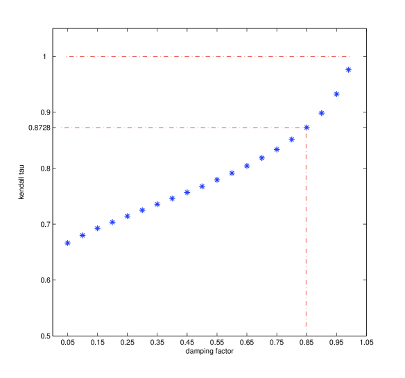
Figure 1: The Kendall Tau metric between $\tilde{\pi}_{T}$ and PageRank of ESCC as a function of the damping factor.

Finally, we would like to note that in the case of quasi-stationarity based centrality measures the first ranking places were occupied by the sites with the internal structure depicted in Figure 2. Therefore, we suggest to use the quasi-stationarity based centrality measures to detect “link farms” and to discover photo albums. It turns out that the quasi-stationarity based centrality measures highlights the sites with structure as in Figure 2 but at the same time the relative ranking of the other sites provided by the standard PageRank with $c=0.85$ is preserved. To illustrate this fact, we give in Table 3 rankings of some sites under different centrality measures. Even though the absolute value of ranking is changing, the relative ranking among these sites is the same for all centrality measures. This indicates that the quasi-stationarity based centrality measures help to discover “link farms” and photo albums and at the same time the ranking of sites of the other type stays consistent with the standard PageRank ranking.

Figure 2: The album like Web site structure

$\pi_{T}(0.85)$ $\bar{\pi}_{T}$ $\tilde{\pi}_{T}$ $\hat{\pi}_{T}$ $\check{\pi}_{T}$ $http://www.inria.fr/$ $1$ $31$ $189$ $105$ $200$ $http://www.loria.fr/$ $13$ $310$ $1605$ $356$ $1633$ $http://www.irisa.fr/$ $16$ $432$ $1696$ $460$ $757$ $http://www-sop.inria.fr/$ $30$ $508$ $1825$ $532$ $1819$ $http://www-rocq.inria.fr/$ $74$ $1333$ $2099$ $1408$ $2158$ $http://www-futurs.inria.fr/$ $102$ $2201$ $2360$ $2206$ $2404$

Table 3: Examples of sites’ rankings

4 Conclusion

In the paper we have proposed centrality measures which can be applied to a reducible graph to avoid the absorbtion problem. In Google PageRank the problem was solved by introduction of uniform random jumps with some probability. Up to the present, there is no clear criterion for the choice this parameter. In the paper we have suggested four quasi-stationarity based parameter-free centrality measures, analyzed them and concluded that they produce approximately the same ranking. Therefore, in practice it is sufficient to compute only one quasi-stationarity based centrality measure. All our theoretical results are confirmed by numerical experiments. The numerical experiments have also showed that the new centrality measures can be applied in spam detection to detect “link farms” and in image search to find photo albums.

Appendix

Here we present a couple of important auxiliary results.

Lemma 1

Let $\bar{T}$ be an irreducible stochastic matrix. And let $T(\varepsilon)=\bar{T}-\varepsilon D$ be a perturbation of $\bar{T}$ such that $T(\varepsilon)$ is substochastic matrix. Then, for sufficiently small $\varepsilon$ the following Laurent series expansion holds

$$[I-T(\varepsilon)]^{-1}=\frac{1}{\varepsilon}X_{-1}+X_{0}+\varepsilon X_{1}+\ldots,$$ (28)

with

$$X_{-1}=\frac{1}{\bar{\pi}D{\bf 1}}{\bf 1}\bar{\pi},$$ (29)

$$X_{0}=(I-X_{-1}D)H(I-DX_{-1}),$$ (30)

where $\bar{\pi}$ is the stationary distribution of $\bar{T}$ and $H=(I-\bar{T}+{\bf 1}\bar{\pi})^{-1}-{\bf 1}\bar{\pi}$ is the deviation matrix.

Proof: The proof of this result is based on the approach developed in [2, 4]. The existence of the Laurent series (28) is a particular case of more general results of [4]. To calculate the terms of the Laurent series, let us equate the terms with the same powers of $\varepsilon$ in the following identity

$$(I-\bar{T}+\varepsilon D)(\frac{1}{\varepsilon}X_{-1}+X_{0}+\varepsilon X_{1}+\ldots)=I,$$

which results in

$$(I-\bar{T})X_{-1}=0,$$ (31)

$$(I-\bar{T})X_{0}+DX_{-1}=I,$$ (32)

$$(I-\bar{T})X_{1}+DX_{0}=0.$$ (33)

From equation (31) we conclude that

$$X_{-1}={\bf 1}\mu_{-1},$$ (34)

where $\mu_{-1}$ is some vector. We find this vector from the condition that the equation (32) has a solution. In particular, equation (32) has a solution if and only if

$$\bar{\pi}(I-DX_{-1})=0.$$

By substituting into the above equation the expression (34), we obtain

$$\bar{\pi}-\bar{\pi}D{\bf 1}\mu_{-1}=0,$$

and, consequently,

$$\mu_{-1}=\frac{1}{\bar{\pi}D{\bf 1}}\bar{\pi},$$

which together with (34) gives (29).

Since the deviation matrix $H$ is a Moore-Penrose generalized inverse of $I-\bar{T}$, the general solution of equation (32) with respect to $X_{0}$ is given by

$$X_{0}=H(I-DX_{-1})+{\bf 1}\mu_{0},$$ (35)

where $\mu_{0}$ is some vector. The vector $\mu_{0}$ can be found from the condition that the equation (33) has a solution. In particular, equation (33) has a solution if and only if

$$\bar{\pi}DX_{0}=0.$$

By substituting into the above equation the expression for the general solution (35), we obtain

$$\bar{\pi}DH(I-DX_{-1})+\bar{\pi}D{\bf 1}\mu_{0}=0.$$

Consequently, we have

$$\mu_{0}=-\frac{1}{\bar{\pi}D{\bf 1}}\bar{\pi}DH(I-DX_{-1})$$

and we obtain (30).

$\Box$

Proposition 11

$$P\left(X_{1}=j|X_{0}=i\wedge\bigwedge_{m=1}^{N}X_{m}\in S\right)=\frac{T_{ij}T^{(N-1)}_{j}{\bf 1}}{T^{(N)}_{i}{\bf 1}}$$

Proof:

$$P\left(X_{1}=j|X_{0}=i\wedge\bigwedge_{m=1}^{N}X_{m}\in S\right)=$$

$$= \frac{P\left(X_{0}=i\wedge X_{1}=j\wedge\bigwedge_{m=2}^{N}X_{m}\in S\right)}{P\left(X_{0}=i\wedge\bigwedge_{m=1}^{N}X_{m}\in S\right)}$$

Denominator:

$$P\left(X_{0}=i\wedge\bigwedge_{m=1}^{N}X_{m}\in S\right)=$$

$$= P\left(X_{0}=i\wedge\bigwedge_{m=1}^{N}\bigvee_{k_{m}\in S}X_{m}=k_{m}\right)=$$

$$= P\left(X_{0}=i\wedge\bigvee_{k_{1}\in S}X_{1}=k_{1}\wedge\bigwedge_{m=2}^{N}\bigvee_{k_{m}\in S}X_{m}=k_{m}\right)=$$

$$= P\left(X_{0}=i\right)\sum_{k_{1}\in S}P\left(X_{1}=k_{1}\wedge\bigwedge_{m=2}^{N}\bigvee_{k_{m}\in S}X_{m}=k_{m}\right)=$$

$$= P\left(X_{0}=i\right)\sum_{k_{1}\in S}P\left(X_{1}=k_{1}|X_{0}=i\right)P\left(\bigwedge_{m=2}^{N}\bigvee_{k_{m}\in S}X_{m}=k_{m}|X_{1}=k_{1}\right)=$$

$$= P\left(X_{0}=i\right)\sum_{k_{1}\in S}P\left(X_{1}=k_{1}|X_{0}=i\right)P\left(\bigvee_{k_{2}\in S}X_{2}=k_{2}\wedge\bigwedge_{m=3}^{N}\bigvee_{k_{m}\in S}X_{m}=k_{m}|X_{1}=k_{1}\right)=$$

$$= P\left(X_{0}=i\right)\sum_{k_{1}\in S}P\left(X_{1}=k_{1}|X_{0}=i\right)\sum_{k_{2}\in S}P\left(X_{2}=k_{2}\wedge\bigwedge_{m=3}^{N}\bigvee_{k_{m}\in S}X_{m}=k_{m}|X_{1}=k_{1}\right)=$$

$$= P\left(X_{0}=i\right)\sum_{k_{1}\in S}P\left(X_{1}=k_{1}|X_{0}=i\right)$$

$$\sum_{k_{2}\in S}P\left(\bigwedge_{m=3}^{N}\bigvee_{k_{m}\in S}X_{m}=k_{m}|X_{2}=k_{2}\wedge X_{1}=k_{1}\right)P\left(X_{2}=k_{2}|X_{1}=k_{1}\right)=$$

$$= P\left(X_{0}=i\right)\sum_{k_{1}\in S}P\left(X_{1}=k_{1}|X_{0}=i\right)$$

$$\sum_{k_{2}\in S}P\left(\bigwedge_{m=3}^{N}\bigvee_{k_{m}\in S}X_{m}=k_{m}|X_{2}=k_{2}\right)P\left(X_{2}=k_{2}|X_{1}=k_{1}\right)=$$

$$= P\left(X_{0}=i\right)\sum_{k_{1}\in S}P\left(X_{1}=k_{1}|X_{0}=i\right)$$

$$\sum_{k_{2}\in S}P\left(\bigwedge_{m=3}^{N}\bigvee_{k_{m}\in S}X_{m}=k_{m}|X_{2}=k_{2}\right)P\left(X_{2}=k_{2}|X_{1}=k_{1}\right)=$$

$$= P\left(X_{0}=i\right)\sum_{k_{2}\in S}P\left(\bigwedge_{m=3}^{N}\bigvee_{k_{m}\in S}X_{m}=k_{m}|X_{2}=k_{2}\right)$$

$$\sum_{k_{1}\in S}P\left(X_{2}=k_{2}|X_{1}=k_{1}\right)P\left(X_{1}=k_{1}|X_{0}=i\right)=$$

$$= P\left(X_{0}=i\right)\sum_{k_{2}\in S}P\left(\bigwedge_{m=3}^{N}\bigvee_{k_{m}\in S}X_{m}=k_{m}|X_{2}=k_{2}\right)P\left(X_{2}=k_{2}|X_{0}=i\right)=$$

$$= P\left(X_{0}=i\right)\sum_{k_{2}\in S}P\left(\bigvee_{k_{3}\in S}X_{3}=k_{3}\wedge\bigwedge_{m=4}^{N}\bigvee_{k_{m}\in S}X_{m}=k_{m}|X_{2}=k_{2}\right)P\left(X_{2}=k_{2}|X_{0}=i\right)=$$

$$= P\left(X_{0}=i\right)\sum_{k_{2}\in S}\sum_{k_{3}\in S}P\left(X_{3}=k_{3}\wedge\bigwedge_{m=4}^{N}\bigvee_{k_{m}\in S}X_{m}=k_{m}|X_{2}=k_{2}\right)P\left(X_{2}=k_{2}|X_{0}=i\right)=$$

$$= P\left(X_{0}=i\right)\sum_{k_{3}\in S}\sum_{k_{2}\in S}P\left(\bigwedge_{m=4}^{N}\bigvee_{k_{m}\in S}X_{m}=k_{m}|X_{3}=k_{3}\wedge X_{2}=k_{2}\right)$$

$$P\left(X_{3}=k_{3}|X_{2}=k_{2}\right)P\left(X_{2}=k_{2}|X_{0}=i\right)=$$

$$= P\left(X_{0}=i\right)\sum_{k_{3}\in S}\sum_{k_{2}\in S}P\left(\bigwedge_{m=4}^{N}\bigvee_{k_{m}\in S}X_{m}=k_{m}|X_{3}=k_{3}\right)$$

$$P\left(X_{3}=k_{3}|X_{2}=k_{2}\right)P\left(X_{2}=k_{2}|X_{0}=i\right)=$$

$$= P\left(X_{0}=i\right)\sum_{k_{3}\in S}P\left(\bigwedge_{m=4}^{N}\bigvee_{k_{m}\in S}X_{m}=k_{m}|X_{3}=k_{3}\right)$$

$$\sum_{k_{2}\in S}P\left(X_{3}=k_{3}|X_{2}=k_{2}\right)P\left(X_{2}=k_{2}|X_{0}=i\right)=$$

$$= P\left(X_{0}=i\right)\sum_{k_{3}\in S}P\left(\bigwedge_{m=4}^{N}\bigvee_{k_{m}\in S}X_{m}=k_{m}|X_{3}=k_{3}\right)P\left(X_{3}=k_{3}|X_{0}=i\right)=\ldots$$

$$\ldots = P\left(X_{0}=i\right)\sum_{k_{N-2}\in S}P\left(\bigwedge_{m=N-1}^{N}\bigvee_{k_{m}\in S}X_{m}=k_{m}|X_{N-2}=k_{N-2}\right)P\left(X_{N-2}=k_{N-2}|X_{0}=i\right)=$$

$$= P\left(X_{0}=i\right)\sum_{k_{N-2}\in S}P\left(\bigvee_{k_{N-1}\in S}X_{N-1}=k_{N-1}\wedge\bigvee_{k_{N}\in S}X_{N}=k_{N}|X_{N-2}=k_{N-2}\right)$$

$$P\left(X_{N-2}=k_{N-2}|X_{0}=i\right)=$$

$$= P\left(X_{0}=i\right)\sum_{k_{N-2}\in S}\sum_{k_{N-1}\in S}P\left(X_{N-1}=k_{N-1}\wedge\bigvee_{k_{N}\in S}X_{N}=k_{N}|X_{N-2}=k_{N-2}\right)$$

$$P\left(X_{N-2}=k_{N-2}|X_{0}=i\right)=$$

$$= P\left(X_{0}=i\right)\sum_{k_{N-2}\in S}\sum_{k_{N-1}\in S}P\left(\bigvee_{k_{N}\in S}X_{N}=k_{N}|X_{N-1}=k_{N-1}\wedge X_{N-2}=k_{N-2}\right)$$

$$P\left(X_{N-1}=k_{N-1}|X_{N-2}=k_{N-2}\right)P\left(X_{N-2}=k_{N-2}|X_{0}=i\right)=$$

$$= P\left(X_{0}=i\right)\sum_{k_{N-2}\in S}\sum_{k_{N-1}\in S}P\left(\bigvee_{k_{N}\in S}X_{N}=k_{N}|X_{N-1}=k_{N-1}\right)$$

$$P\left(X_{N-1}=k_{N-1}|X_{N-2}=k_{N-2}\right)P\left(X_{N-2}=k_{N-2}|X_{0}=i\right)=$$

$$= P\left(X_{0}=i\right)\sum_{k_{N-1}\in S}P\left(\bigvee_{k_{N}\in S}X_{N}=k_{N}|X_{N-1}=k_{N-1}\right)$$

$$\sum_{k_{N-2}\in S}P\left(X_{N-1}=k_{N-1}|X_{N-2}=k_{N-2}\right)P\left(X_{N-2}=k_{N-2}|X_{0}=i\right)=$$

$$= P\left(X_{0}=i\right)\sum_{k_{N-1}\in S}P\left(\bigvee_{k_{N}\in S}X_{N}=k_{N}|X_{N-1}=k_{N-1}\right)P\left(X_{N-1}=k_{N-1}|X_{0}=i\right)=$$

$$= P\left(X_{0}=i\right)\sum_{k_{N-1}\in S}\sum_{k_{N}\in S}P\left(X_{N}=k_{N}|X_{N-1}=k_{N-1}\right)P\left(X_{N-1}=k_{N-1}|X_{0}=i\right)=$$

$$= P\left(X_{0}=i\right)\sum_{k_{N}\in S}\sum_{k_{N-1}\in S}P\left(X_{N}=k_{N}|X_{N-1}=k_{N-1}\right)P\left(X_{N-1}=k_{N-1}|X_{0}=i\right)=$$

$$= P\left(X_{0}=i\right)\sum_{k_{N}\in S}P\left(X_{N}=k_{N}|X_{0}=i\right)=$$

$$= \sum_{k_{N}=1}^{n_{T}}T^{(N)}_{ik_{N}}P\left(X_{0}=i\right)=$$

$$= T^{(N)}_{i}{\bf 1}P\left(X_{0}=i\right)=$$

$$P\left(X_{0}=i\wedge\bigwedge_{m=1}^{N}X_{m}\in S\right)=T^{(N)}_{i}{\bf 1}P\left(X_{0}=i\right)$$

Numerator:

$$P\left(X_{0}=i\wedge X_{1}=j\wedge\bigwedge_{m=2}^{N}X_{m}\in S\right)=$$

$$= P\left(\bigwedge_{m=2}^{N}\bigvee_{k_{m}\in S}X_{m}=k_{m}\right)P\left(X_{1}=j|X_{0}=i\right)P\left(X_{0}=i\right)=$$

$$= T_{ij}T^{(N-1)}_{j}{\bf 1}P\left(X_{0}=i\right)=$$

$$P\left(X_{0}=i\wedge X_{1}=j\wedge\bigwedge_{m=2}^{N}X_{m}\in S\right)=T_{ij}T^{(N-1)}_{j}{\bf 1}P\left(X_{0}=i\right)$$

$\Box$

References

• [1] S. Abiteboul, M. Preda, and G. Cobena, “Adaptive on-line page importance computation”, in Proceedings of the 12 International World Wide Web Conference, Budapest, 2003.
• [2] K. Avrachenkov, Analytic Perturbation Theory and its Applications, PhD thesis, University of South Australia, 1999.
• [3] K. Avrachenkov, D. Nemirovsky, and N. Osipova. “Web Graph Analyzer Tool”. In Proceedings of the IEEE ValueTools conference, 2006.
• [4] K. Avrachenkov, M. Haviv and P.G. Howlett, “Inversion of analytic matrix functions that are singular at the origin”, SIAM Journal on Matrix Analysis and Applications, v. 22(4), pp.1175-1189, 2001.
• [5] K. Avrachenkov, N. Litvak and K.S. Pham, “A singular perturbation approach for choosing PageRank damping factor”, preprint, available at http://arxiv.org/abs/math.PR/0612079, 2006.
• [6] P. Boldi, M. Santini, and S. Vigna, “PageRank as a function of the damping factor”, in Proceedings of the 14 World Wide Web Conference, New York, 2005.
• [7] A. Broder, R. Kumar, F. Maghoul, P. Raghavan, S. Rajagopalan, R. Stata, A. Tomkins and J. Wiener, “Graph structure in the Web”, Computer Networks, v. 33, pp.309-320, 2000.
• [8] P. Chen, H. Xie, S. Maslov, and S. Redner, “Finding scientific gems with Google’s PageRank algorithm”, Journal of Informetrics, v.1, pp.8–15, 2007.
• [9] J. N. Darroch and E. Seneta, “On Quasi-Stationary Distributions in Absorbing Discrete-Time Finite Markov Chains”, Journal of Applied Probability, v. 2(1), pp.88-100, 1965.
• [10] S. Dill, R. Kumar, K. McCurley, S. Rajagopalan, D. Sivakumar, and A. Tomkins, “Self-similarity in the Web”, ACM Trans. Internet Technol., 2 (2002), pp. 205–223.
• [11] E.A. van Doorn, “Quasi-stationary distributions and convergence to quasi-stationarity of birth-death processes”, Advances in Applied Probability, v. 23(4), pp. 683-700, 1991.
• [12] W.J. Ewens, “The diffusion equation and pseudo-distribution in genetics”, J.R. Statist. Soc. B, v. 25, pp. 405-412, 1963.
• [13] J. Kleinberg, “Authoritative sources in a hyperlinked environment”, Journal of ACM, v. 46, pp.604-632, 1999.
• [14] I. Kontoyiannis, and S. P. Meyn, “Spectral theory and limit theorems for geometrically ergodic Markov processes”, Ann. Appl. Probab., v. 13, no. 1, pp. 304362, 2003.
• [15] R. Kumar, P. Raghavan, S. Rajagopalan, D. Sivakumar, A. Tompkins and E. Upfal, “The Web as a graph”, PODS’00: Proceedings of the nineteenth ACM SIGMOD-SIGACT-SIGART Symposium on Principles of Database Systems, pp. 1-10, 2000.
• [16] A. N. Langville and C. D. Meyer, “Deeper Inside PageRank”, Internet Math., 1 (2004), pp. 335–400; also available online at http://www4.ncsu.edu/$\!{}_{{}^{\sim}}\!$anlangvi/.
• [17] A. N. Langville and C. D. Meyer, “Updating PageRank with iterative aggregation”, in Proceedings of the 13th World Wide Web Conference, New York, 2004.
• [18] A.N. Langville and C.D. Meyer, “Google’s PageRank and Beyond: The Science of Search Engine Rankings”, Princeton University Press, 2006.
• [19] R. Lempel and S. Moran, “The stochastic approach for link-structure analysis (SALSA) and the TKC effect”, Computer Networks, v. 33, pp. 387-401, 2000.
• [20] C.D. Moler and K.A. Moler, “Numerical Computing with MATLAB”, SIAM , 2003.
• [21] L. Page, S. Brin, R. Motwani and T. Winograd, “The pagerank citation ranking: Bringing order to the web”, Stanford Technical Report, 1998.
• [22] E. Seneta, “Non-negative matrices and Markov chains”, Springer, 1973.