Critical Behavior in the Gravitational Collapse of a Scalar Field with Angular Momentum in Spherical Symmetry

Abstract

We study the critical collapse of a massless scalar field with angular momentum in spherical symmetry. In order to mimic the effects of angular momentum we perform a sum of the stress-energy tensors for all the scalar fields with the same eigenvalue $l$ of the angular momentum operator and calculate the equations of motion for the radial part of these scalar fields. We have found that the critical solutions for different values of $l$ are discretely self-similar (as in the original $l=0$ case). The value of the discrete, self-similar period, $\Delta_{l}$, decreases as $l$ increases in such a way that the critical solution appears to become periodic in the limit. The mass scaling exponent, $\gamma_{l}$, also decreases with $l$.

I Introduction

Most studies of black hole critical phenomena (see Gundlach:1999cu , Gundlach:2002sx for reviews) to date (or related phenomena in other sets of nonlinear evolution equations) have been performed assuming spherical symmetry as a simplifying assumption (exceptions are Abrahams:wa , Liebling:2002qp and more recently Choptuik:2003ac ). This simplification has been adopted in most cases because accurate calculation of Type II critical solutions—which exhibit structure at all scales due to their self-similar nature—requires great computational resources. Since spherically symmetric spacetimes do not allow for angular momentum, very little is currently known about the role of angular momentum in critical collapse. For a few cases, most notably the Type II solutions found in spherically symmetric collapse of a massless scalar field Garfinkle:1998tt , or certain types of perfect fluid Gundlach:1997nb , Gundlach:1999cw , perturbative calculations about the spherical critical solutions suggest that non-spherical modes, including those contributing to net angular momentum, are damped as one approaches criticality. In particular in Garfinkle:1998tt , Gundlach:1997nb and Gundlach:1999cw using second order perturbation theory it was predicted that the angular momentum of the black holes produced should have the following dependence as a function of the critical parameter $p$:

$$\vec{L}_{\rm{BH}}=\vec{L}_{0}\left(p-p^{\star}\right)^{\mu},$$ (1)

where $\vec{L}_{0}$ is family-dependent and $\mu$ is a universal scaling exponent satisfying $\mu>2\gamma$ ($\gamma$ being the scaling exponent for the black hole mass). Specifically, it was suggested that $\mu\approx 0.76$ for the scalar field case, whereas the computations indicated that $\mu$ would depend on the equation of state for perfect fluid collapse. These calculations thus suggest that, at least for small deviations from spherical symmetry, the resulting solutions on the verge of black hole formation should remain spherically symmetric in non-symmetric collapse. We also note that an axisymmetric numerical relativity code has been developed hlcp to study non-perturbatively some effects of angular momentum in the critical collapse of a scalar field. Interestingly, the results found for $\Delta$ and $\gamma$ in the case of a complex scalar field with principal azimuthal “quantum number”, $m=1$ are very close to the results we find in our model for $l=1$, as described in Sec. III.

Here a different approach is taken. Maintaining spherical symmetry, the equations of motion for a massless scalar field are modified by effective terms which mock up some of the effects of angular momentum. As described below, the procedure amounts to performing an angular average over the matter field variables—similar to that done in Rein:1998uf , Olabarrieta:2001wy and Ventrella:2003fu —and results in an entire family of models, parameterized by a principal angular “quantum number”, $l$ (we will generally restrict $l$ to take on non-negative integer values, although real-valued $l$’s are also formally possible). We note that since the models remain spherically symmetric, we cannot use them to address the validity of the perturbative calculations mentioned above (e.g. equation (1)). Nonetheless, we find interesting results that may shed some light on the effects of angular momentum near the black hole threshold.

Some of the main results that have been found are as follows. First, each value of the angular momentum parameter $l$ apparently defines a distinct critical solution. For $l<10$, these solutions are found to be discretely self similar, with values of the echoing exponent, $\Delta_{l}$, that rapidly decrease (approximately exponentially) as $l$ increases. As a result, for large values of $l$, and for the time scales for which we are able to dynamically evolve near criticality, the threshold solutions become approximately periodic. In addition, and as expected for Type II solutions, we find that for $l<7$ the masses of the black holes formed follow power laws. As with the echoing exponents, for increasing values of $l$ it is found that the mass-scaling exponent, $\gamma_{l}$, rapidly decreases, again approximately exponentially in $l$.

The remainder of this paper is structured as follows. In the following section we describe the recipe used to calculate the effective equations of motion, along with the regularity and boundary conditions imposed in the solution of these equations. In Sec. III we briefly describe the numerical code, the way the solutions have been analyzed, and then provide a summary of the results obtained for varying values of $l$. Throughout this paper we use units such that the universal gravitational constant, $G$, and the speed of light in vacuum, $c$, are both unity.

II Equations of Motion

II.1 Equations

In order to derive equations of motion, scalar fields of the following form are considered:

$$\Psi^{m}_{l}(t,r,\theta,\phi) = \psi^{(l)}(t,r)\,Q_{lm}(\theta,\phi),$$ (2)

$$m=-l,-l+1,\cdots,l-1,l,$$

where $Q_{lm}(\theta,\phi)$ are normalized real eigenfunctions of the angular part of the flatspace Laplacian with eigenvalue $l(l+1)$, and the index $m$ labels the $2l+1$ distinct orthonormal eigenfunctions for a given value of $l$. More explicitly:

$$Q_{lm}=\left\{\begin{array}[]{l l}Y_{l0}&{\rm for}\quad m=0,\\ \frac{1}{\sqrt{2}}\left(Y_{lm}+(-1)^{m}Y_{l-m}\right)&{\rm for}\quad m>0,\\ \frac{1}{i\sqrt{2}}\left(Y_{l|m|}-(-1)^{|m|}Y_{l-|m|}\right)&{\rm for}\quad m<0,\end{array}\right.$$ (3)

where $Y_{lm}\left(\theta,\phi\right)$ are the regular spherical harmonics. By construction, the scalar fields $\Psi^{m}_{l}$ are not, in general, spherically symmetric and we therefore do not study their collapse directly. Instead, our strategy is to find effective equations for the single $(t,r)$-dependent quantity $\psi^{(l)}(t,r)$, which we hereafter denote simply by $\psi$. To do so, for a specific value of $l$, we consider the stress-energy tensors for the $2l+1$ fields $\Psi^{m}_{l}$:

$$T^{(lm)}{}_{ab}=\nabla_{a}\Psi^{m}_{l}\nabla_{b}\Psi^{m}_{l}-\frac{1}{2}g_{ab}(\nabla^{c}\Psi^{m}_{l}\nabla_{c}\Psi^{m}_{l}),$$ (4)

where $g_{ab}$ is the metric of the spacetime and $\nabla_{a}$ is the metric-compatible covariant derivative. Again by construction, and as is proven in Appendix A, the sum of these stress tensors

$${\mathcal{T}}^{(l)}{}_{ab}=\sum_{m}T^{(lm)}{}_{ab},$$ (5)

is spherically symmetric, and thus depends only on $\psi(t,r)$, $l$, and the metric $g_{ab}$. We can now compute the effective equation of motion for the field, $\psi(t,r)$, using the fact that the divergence of the total stress energy tensor is zero, as is also proven in Appendix A:

$$g^{ac}\nabla_{c}{\mathcal{T}}^{(l)}{}_{ab}=0\,.$$ (6)

The equations for the geometric variables are determined from the $3+1$ decomposition of the Einstein field equations. For the current study we adopt Schwarzschild-like (polar-areal) coordinates, in which the metric takes the form:

$$ds^{2}=-\alpha^{2}(t,r)dt^{2} + a^{2}(t,r)dr^{2}$$ (7)

$$+ r^{2}d\theta^{2}+r^{2}\sin^{2}{\theta}d\phi^{2}\,.$$

Here $\alpha(t,r)$ is the lapse function and $a(t,r)$ is the only non-trivial components of the 3-metric (both $\alpha$ and $a$ are positive functions). Using this metric, the non zero components of the stress-energy tensor for a general value of $l$ are

$${\mathcal{T}}^{(l)}{}^{t}{}_{t} = -\frac{(2l+1)}{8\pi}\left[\frac{1}{a^{2}}\left(\Pi^{2}+\Phi^{2}\right)+l(l+1)\frac{\psi^{2}}{r^{2}}\right],$$ (8)

$${\mathcal{T}}^{(l)}{}^{t}{}_{r} = -\frac{(2l+1)}{8\pi}\frac{2}{a\alpha}\,\Pi\,\Phi,$$ (9)

$${\mathcal{T}}^{(l)}{}^{r}{}_{r} = \frac{(2l+1)}{8\pi}\left[\frac{1}{a^{2}}\left(\Pi^{2}+\Phi^{2}\right)-l(l+1)\frac{\psi^{2}}{r^{2}}\right],$$ (10)

$${\mathcal{T}}^{(l)}{}^{\theta}{}_{\theta} = {\mathcal{T}}^{(l)}{}^{\phi}{}_{\phi}=\frac{(2l+1)}{8\pi a^{2}}\left(\Pi^{2}-\Phi^{2}\right)\,,$$ (11)

and the stress-energy trace is

$${\mathcal{T}}^{(l)} \equiv {\mathcal{T}}^{(l)}{}^{i}{}_{i}$$ (12)

$$= \frac{(2l+1)}{8\pi}\left[\frac{2}{a^{2}}\left(\Pi^{2}-\Phi^{2}\right)-2l(l+1)\frac{\psi^{2}}{r^{2}}\right]\!.$$

In the above expressions, we have made use of the auxiliary variables, $\Phi$ and $\Pi$, defined as follows:

$$\Phi\left(t,r\right) = \frac{\partial\psi}{\partial r},$$ (13)

$$\Pi\left(t,r\right) = \frac{a}{\alpha}\frac{\partial\psi}{\partial t}.$$ (14)

The dynamical equations of motion for these fields, which follow from the definition of $\Phi$ as well as the wave equation for $\psi$ (which in turn can be derived from the vanishing of the divergence of the total stress tensor (6)) are then:

$$\frac{\partial\Phi}{\partial t} = \frac{\partial}{\partial r}\left(\frac{\alpha}{a}\Pi\right),$$ (15)

$$\frac{\partial\Pi}{\partial t} = \frac{1}{r^{2}}\frac{\partial}{\partial r}\left(r^{2}\frac{\alpha}{a}\Phi\right)-l(l+1)a\alpha\frac{\psi}{r^{2}}\,.$$ (16)

Note that the dependence of these equations on $l$ is only through the last term in equation (16) which is proportional to $l(l+1)/r^{2}$. This term can be thought of as the field-theoretic extension of an analogous term due to the angular momentum potential, $l^{2}/r^{2}$, in the 1-dimensional reduced problem of a particle moving in a central potential.

As mentioned above, equations for the geometric variables result from the $3+1$ decomposition of the field equations, as well as from our choice of coordinates. Specifically, we have the following

$$\frac{1}{a}\frac{\partial a}{\partial r} = \frac{(2l+1)}{2}r\left(\Pi^{2}+\Phi^{2}+l(l+1)\frac{a^{2}}{r^{2}}\psi^{2}\right)$$ (17)

$$- \frac{a^{2}-1}{2r},$$

$$\frac{1}{\alpha}\frac{\partial\alpha}{\partial r} = \frac{(2l+1)}{2}r\left(\Pi^{2}+\Phi^{2}-l(l+1)\frac{a^{2}}{r^{2}}\psi^{2}\right)$$ (18)

$$+ \frac{a^{2}-1}{2r},$$

$$\frac{\partial a}{\partial t} = (2l+1)r\alpha\Pi\Phi.$$ (19)

Equation (17) is the Hamiltonian constraint, which is used to determine the 3-metric component, $a$. Similarly, the slicing condition (18) fixes the lapse function $\alpha$ at each instant of time, and is often known as the polar slicing condition. It can be derived from the demand that ${\rm Tr}\left(K_{ab}\right)=K^{r}{}_{r}+K^{\theta}{}_{\theta}+K^{\phi}{}_{\phi}=K^{r}{}_{r}+2K^{\theta}{}_{\theta}=0$, for all times. The Hamiltonian constraint and slicing condition, with appropriate regularity and boundary conditions, completely fix the geometric variables in this coordinate system. Equation (19) is an extra equation derived from the definition of $K^{r}{}_{r}$ and the momentum constraint. In our numerical solutions, it is used as a gauge of the accuracy of our calculations, as well as to provide a replacement for the Hamiltonian constraint in certain strong field instances where the numerical constraint solver fails. In addition, we compute the mass aspect function, $M(t,r)$,

$$M(t,r)=\frac{r}{2}\left(1-\frac{1}{a^{2}}\right),$$ (20)

which serves as a valuable diagnostic quantity in our calculations. The value of this function as $r\to\infty$ agrees with the ADM mass, and more generally, in a vacuum region of spacetime, measures the amount of (gravitating) mass contained within the 2-sphere of radius $r$ at time $t$. Moreover, $2M(t,r)/r$ is useful since its value approaches $1$ when a trapped surface is developing and hence (modulo cosmic censorship), a black hole would form in the spacetime being constructed. We note that, as is the case with the usual Schwarzschild coordinates for a spherically symmetric black hole, polar-areal coordinates cannot penetrate apparent horizons, and in fact become singular as they come “close to” black-hole regions of spacetime, where $2M(t,r)/r\to 1$. This fact does not present a problem in the study of critical behavior in our models, since the critical solutions per se have $\max_{r}\left\{2M(t,r)/r\right\}$ bounded away from $1$.

II.2 Regularity and Boundary Conditions

In addition to the above equations of motion, appropriate regularity and boundary conditions are needed. At the origin, $r=0$, regularity is enforced via

$$a(t,0) = 1,$$ (21)

$$\frac{\partial a}{\partial r}(t,0) = 0,$$ (22)

$$\frac{\partial\alpha}{\partial r}(t,0) = 0,$$ (23)

$$\psi(t,0) = O(r^{l}),$$ (24)

$$\Pi(t,0) = O(r^{l}),$$ (25)

$$\Phi(t,0) = \left\{\begin{array}[]{lll}O(r^{l-1})&\hbox{\rm for}&l\geq 1,\\ O(r)&\hbox{\rm for}&l=0.\end{array}\right.$$ (28)

In the continuum, our equations of motion are to be solved as a pure Cauchy problem, on the domain $t\geq 0$, $r\geq 0$, with boundary conditions at spatial infinity given by asymptotic flatness (i.e. that the matter fields vanish, and that the metric becomes that of Minkowski spacetime, as $r\to\infty$). Computationally, we solve an approximation to this problem on a finite spatial domain $0\leq r\leq r_{\rm max}$, where $r_{\rm max}$ is some arbitrary outer radius chosen sufficiently large that we are confident that the numerical results do not depend significantly on its precise value. At the outer boundary, then, the following condition for $\alpha$ is imposed:

$$\alpha(t,r_{\rm max})\ a(t,r_{\rm max})=1.$$ (29)

This can be viewed as simply providing a convenient normalization for $\alpha$, since given a solution, $\alpha$, of the slicing equation (18), $k\alpha$ is also a solution, where $k$ is an arbitrary positive constant. We note that although we have used (29) in order to perform the calculations, a different normalization convention—i.e. a different, and time dependent, choice of $k$—has been used in order to perform the analysis of the solutions. Specifically, in the analysis we have used central proper time $T$ defined by:

$$T=\int^{T}_{0}\alpha({\tilde{t}},0)\,d{\tilde{t}}\,.$$ (30)

This definition of time has a natural geometrical interpretation since $r=0$ is invariantly defined by the symmetry of the spacetime. For the scalar field variables, $\Pi$ and $\Phi$, approximate outgoing-radiation boundary conditions (Sommerfeld conditions) are used:

$$\frac{\partial\Phi}{\partial t}(t,r_{\rm max})+\frac{\partial\Phi}{\partial r}(t,r_{\rm max})+\frac{\Phi(t,r_{\rm max})}{r_{\rm max}} = 0,$$ (31)

$$\frac{\partial\Pi}{\partial t}(t,r_{\rm max})+\frac{\partial\Pi}{\partial r}(t,r_{\rm max})+\frac{\Pi(t,r_{\rm max})}{r_{\rm max}} = 0.$$ (32)

An important point in the derivation of the equations of motion is the fact that the eigenfunctions in (2) are discrete and the allowable values of $l$ are only non-negative integers. Once the equations are obtained we have relaxed that constraint and have allowed $l$ to take non-negative real values. The solutions corresponding to non-integer values of $l$ would have some degree of irregularity at the origin depending on the particular value of $l$ chosen. This implies that only some finite number of derivatives with respect to $r$ will be defined at $r=0$. In our particular numerical implementation, which assumes that second derivatives of the variables are defined, we have been able to study the evolution of these systems as long as $l>3$.

III Results

III.1 Numerics

We solve equations (15), (16) for the scalar field gradients, equations (17), (18) for the geometry, and use (13) to reconstruct the field $\psi$. The system is approximated using second order centered finite difference techniques, and coded using RNPL rnpl . Numerical dissipation of the Kreiss-Oliger KO variety was included to damp high frequency modes, and it should be noted that this particular type of dissipation is added at sub-truncation error order, so does not affect the overall accuracy of the scheme as the mesh spacing tends to 0. For the current computations, the damping terms were most useful in regularizing the truncation error estimation procedure that occurs when adaptive mesh refinement (AMR) techniques are used. It was also crucial to impose the correct leading-order regularity conditions close to the origin, $r=0$ (equations (25)-(28)), in order to keep the solution regular during the evolutions. Most of the calculations were done on a fixed uniform spatial grid $r_{j}=(j-1)\Delta r$, $j=1,2,\cdots,J$, $J=1+r_{\rm max}/\Delta r$ with a typical number of grid points $J=1025$, and the outer boundary of the computational domain typically at $r_{\rm max}=100$. For small values of the angular momentum parameter—specifically for $l\leq 2$—an AMR algorithm based on that described in Choptuik:jv was used.

III.2 Families of Initial Data

Our study involved the evolution of $6$ different one parameter families of initial data, each defined by an initial profile $\psi(0,r)$ as listed in Table 1, with specific values of the parameters appearing in the profile definitions as given in Table 2. In addition to $\psi(0,r)$, we need to provide $\Pi(0,r)$ to complete the specification of the initial data. In all cases we chose $\Pi(0,r)$ to produce an approximately in-going pulse at the initial time:

$$\Pi(0,r)=\Phi(0,r)=\frac{\partial\psi}{\partial r}(0,r).$$ (33)

Family	Form of initial data, $\psi(0,r)$	$p$
(a)	$A\,\exp\left(-(r-r_{0})^{2}/\sigma^{2}\right)$	$A$
(b)	$-2A\,(r-r_{0})/\sigma^{2}\exp\left(-(r-r_{0})^{2}/\sigma^{2}\right)$	$A$
(c)	$A\,r^{2}\left({\mathrm{atan}}(r-r_{0})-{\mathrm{atan}}(r-r_{0}-\sigma)\right)$	$A$

Table 1: Families of initial data and the parameter $p$ that is tuned to generate a critical solution.

As previously mentioned, all of the initial data families listed in Table 1 have a single free parameter, $p$, and, as is the usual case in studies of black hole critical phenomena, for any given family we observe two different final states in the evolution, depending on the value of $p$. For values of $p>p^{\star}$ the maximum value of $2M(t,r)/r$ approaches $1$ implying that an apparent horizon is about to form. On the other hand if $p<p^{\star}$ the scalar field completely disperses, and leaves (essentially) flat spacetime in its wake. The solution that arises as $p\to p^{\star}$ then represents the threshold of black hole formation and, by definition, is the critical solution. We note that these critical solutions are not $t\to\infty$ end-states of evolution; rather they persist for only a finite amount of time, and, in fact, are unstable, heuristically representing an infinitely fine-tuned balance between dispersal and gravitational collapse.

Initial Data (F)	Family	Parameters
1	(a)	$r_{0}=70.0$,  $\sigma=5.00$
2	(b)	$r_{0}=70.0$,  $\sigma=5.00$
3	(c)	$r_{0}=70.0$,  $\sigma=5.00$
4	(a)	$r_{0}=40.0$,  $\sigma=10.0$
5	(a)	$r_{0}=40.0$,  $\sigma=5.00$
6	(a)	$r_{0}=70.0$,  $\sigma=10.0$

Table 2: Initial data used in our investigations. The family labels are defined in Table I.

III.3 Analysis

We have calculated $p^{\star}$ for the different families of initial data described above, and for different values of $l$, via bisection (binary search), tuning $p$ in each case to a typical precision of $\left(p-p^{\star}\right)/p\approx 10^{-15}$ (which is close to machine precision using 8-byte real floating point arithmetic).

As in the case for $l=0$ (where the equations of motion reduce to those for a single, non-interacting massless scalar field, as studied in Choptuik:jv ), the critical solutions for values of $l\leq 9.5$ are apparently discretely self similar (DSS). DSS spacetimes are scale-periodic, meaning that any non-dimensional quantity, $Z$, obeys the following equation for some specific values of the parameters $\Delta$ and $T^{\star}$:

$$Z\left((T-T^{\star}),r\right)=Z\left(e^{n\Delta}(T-T^{\star}),e^{n\Delta}r\right),$$ (34)

where $T$ is central proper time as defined by (30), and $T^{\star}$ is the “accumulation time” of the self-similar solution. In (34) the integer $n$ denotes the “echo” number. We also note that due to the discrete $\psi\to-\psi$ invariance that is exhibited both by the equations of motion as well as the critical solutions themselves, if $\Delta$ is the echoing exponent for which formula (34) is satisfied with $Z(T,r)\equiv\psi(T,r)$, then the geometric quantities $a(T,r)$, $\alpha(T,r)$, $2M(T,r)/r$ obey (34) with an echoing exponent $\Delta/2$.

In order to extract $\Delta$ from our calculations, we use the observation that certain geometric quantities will achieve (locally) extremal values on the spatial domain at discrete central proper times $T_{n}$ given by

$$T_{n}-T^{\star}=\left(T_{0}-T^{\star}\right)e^{n\Delta/2}$$ (35)

where $T_{0}$ is the time at which one starts counting the echoes. Specifically, $\Delta$ and $T^{\star}$ have been computed by a least squares fit for the times $T_{n}$ at which $\max_{r}\left\{2M(t,r)/r\right\}$ achieves a local maximum in time, i.e. by minimizing:

$$\chi^{2}=\sum_{n=1}^{N}\left\{T_{n}-T_{0}e^{n\Delta/2}+T^{\star}\left(e^{n\Delta/2}-1\right)\right\}^{2}.$$ (36)

$l$	$\Delta_{l}$	$\gamma_{l}$
0	3.43 $\pm$ 0.05	0.376 $\pm$ 0.003
1	0.460 $\pm$ 0.002	0.119 $\pm$ 0.001
2	0.119 $\pm$ 0.003	0.0453 $\pm$ 0.0002
3	0.039 $\pm$ 0.001	0.020 $\pm$ 0.001
3.5	0.0224 $\pm$ 0.0009	0.0127 $\pm$ 0.0008
4	0.0132 $\pm$ 0.0008	0.0082 $\pm$ 0.0008
4.5	0.0077 $\pm$ 0.0007	0.0052 $\pm$ 0.0006
5	0.0044 $\pm$ 0.0007	0.0033 $\pm$ 0.0005
5.5	0.0026 $\pm$ 0.0006	0.0020 $\pm$ 0.0005
6	0.0015 $\pm$ 0.0005	0.0013 $\pm$ 0.0005
6.5	0.0009 $\pm$ 0.0005	0.0008 $\pm$ 0.0005
7	0.0006 $\pm$ 0.0004	-
7.5	0.0004 $\pm$ 0.0004	-
8	0.0003 $\pm$ 0.0004	-
8.5	0.0002 $\pm$ 0.0003	-
9	0.0002 $\pm$ 0.0004	-
9.5	0.0002 $\pm$ 0.0003	-

Table 3: Summary of the properties of the critical solutions computed for different values of $l$. Note that both the echoing exponents, $\Delta_{l}$, and the mass scaling exponents, $\gamma_{l}$, rapidly decrease as $l$ increases. Quoted errors have been estimated from the variation in values computed across the different families of initial data. Values of $\Delta_{l}$ have been calculated using central proper time normalization of the lapse function, which is the natural normalization for type-II critical behavior. For $l>6.5$ we have not been able to calculate $\gamma_{l}$ due to lack of numerical precision. Note that the $l=0$ data agree with the original values calculated in Choptuik:jv , and that the $l=1$ data agree with values calculated in Liebling:1999ke and Husa:2000kr using models of completely different origin.

III.4 Results

Table 3 summarizes the values of $\Delta_{l}$ we have estimated using this procedure; the data are also graphed in Fig. 1. Again, note that the reported values for $\Delta_{l}$ have been calculated using central proper time $T$ instead of proper time at infinity (the parameterization used in the numerical evolutions per se). Also the reported uncertainties have been estimated from the deviations in the $\Delta_{l}$ values computed across the the six different families of initial data. The first entry in Table 3 ($l=0$) corresponds to the original case studied in Choptuik:jv . The second one ($l=1$) is apparently the same solution found for the self-gravitating collapse of an $SO(3)$ non-linear $\sigma$ model, assuming a hedgehog ansatz Husa:2000kr , Liebling:1999ke . Interestingly, the values for $\Delta_{1}$ and $\gamma_{1}$ also agree quite well with the values obtained from the study of the axisymmetric collapse of a complex-valued scalar field with azimuthal quantum number $m=1$ hlcp , where values $\Delta\approx 0.42$ and $\gamma\approx 0.11$ are quoted. However, in the model considered in hlcp , the overall solution is clearly different because it is not spherically symmetric. The remainder of the solutions (for the other values of $l$) are, to the best of our knowledge, new.

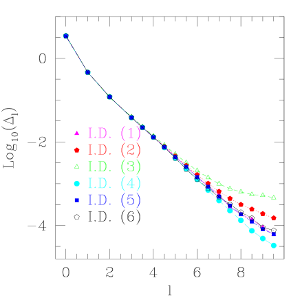
Figure 1: Values of ${\mathrm{log}_{10}}\left(\Delta_{l}\right)$ versus $l$. In this figure we can see that $\Delta_{l}$ decreases almost exponentially with $l$. The different lines represent different families of initial data. Assuming universality, the differences between the values calculated for the different families provides one measure of error in our determination of $\Delta_{l}$.

Systems exhibiting type II critical behavior, where the critical solution is self-similar, generally also exhibit power-law scaling of dimensionful quantities in near-critical evolutions. For example, we can expect the black hole mass, $M_{\rm BH}$, to scale as

$$M_{\rm BH}\sim C\left(p-p^{\star}\right)^{\gamma_{l}}$$ (37)

for super-critical evolutions as $p\to p^{\star}$ . Here $C$ is a constant that depends on the family of initial data while $\gamma_{l}$ is a universal exponent for each value of $l$, i.e. independent of the specific initial data family used to generate the critical solution. We have observed such scaling in at least some of our computations, but, following Garfinkle and Duncan Garfinkle:1998va have found it more convenient to extract $\gamma_{l}$ by monitoring the maximum value of the trace of the stress tensor, ${\cal T}$, which, from the Einstein equations, is proportional to the maximum value of the Ricci curvature. On dimensional grounds $\cal T$ (defined by (12)) and $R$ should both scale with an exponent $-2\gamma$. This technique has the advantage of being more precise than a strategy based directly on (37) since we can calculate the trace of the stress-energy more accurately than the mass of the black hole formed, and can perform the computation using sub-critical evolutions, where the gradients of field variables generally do not become as large as those in the super-critical cases. The values of $\gamma_{l}$ as a function of $l$ are listed in Table 3 and are plotted in Fig. 2.

Figure 2: Values of ${\mathrm{log}_{10}}\left(\gamma_{l}\right)$ versus $l$, where $\gamma_{l}$ is the scaling exponent defined by (37). As for the case of the echoing exponent, $\Delta_{l}$, $\gamma_{l}$ also decreases approximately exponentially with $l$. We note that due to lack of numerical precision we can only reliably compute $\gamma_{l}$ for $l\leq 6.5$

As is characteristic of type-II critical solutions exhibiting discrete self-similarity, $2M(t,r)/r$ oscillates at higher frequencies and on smaller spatial scales during the course of an evolution in the critical regime. As has already been noted, as $l$ increases, the echoing exponent $\Delta_{l}$ decreases rapidly. This can be observed in Fig. 3 where the evolution of the maximum in $r$ is shown as a function of time for four different values of $L$.

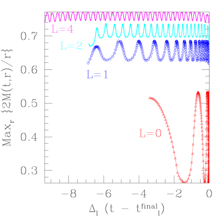
Figure 3: Evolution in time of the maximum in $r$ of the function $2M(t,r)/r$ for four different critical solutions with increasing value of $l$ ($l=0$, $l=1$, $l=2$ and $l=4$). The plot shows the evolution during the period of time when each solution shows discrete self similarity. The time coordinate is rescaled by $\Delta_{l}$ for visualization purposes and is shifted so that the function values coincide at $t=0$. We note how the solutions tend to periodicity with increasing values of $l$.

In addition, also in Fig. 3, we observe that the maximum and minimum values between which the spatial maximum of $2M(t,r)/r$ oscillates increase with $l$ (this fact is shown for all values of $l$ in Fig. 4) indicating that the critical solutions are becoming increasingly relativistic as the angular momentum barrier becomes more pronounced. The amplitude of the oscillations between these extremal values decreases since $\min_{r}\left\{2M(t,r)/r\right\}$ increases more rapidly than $\max_{r}\left\{2M(t,r)/r\right\}$ (see Fig. 4).

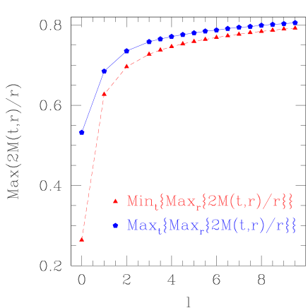
Figure 4: $\max_{t}\left\{\max_{r}\left\{2M(t,r)/r\right\}\right\}$ in the critical regime as a function of $l$ (solid line) and the same for $\min_{t}\left\{\max_{r}\left\{2M(t,r)/r\right\}\right\}$ (dashed line). We see how both the maximum and minimum values of $2M/r$ increase with $l$. On the other hand the amplitude of oscillation, given by their difference, apparently tends to zero with increasing $l$.

The assumption that the critical solutions are independent of the initial family of initial data implies that the spatial profiles at the same moment during the oscillation for two different families of initial data are the same up to some rescaling of the radial coordinate. In Fig. 5 we show a check of the universality of the spatial profile for the solutions computed with $l=9$. Specifically we compare the spatial profiles at times $T_{n}$, times at which the local maximum in time is achieved during criticality, for different families $F$ of initial data $F=1,...,6$ given in Table 2. In order to compare profiles we rescaled the radial coordinate by a constant $K_{F}$, which depends on the family of initial data. These constants are chosen in such a way that the $\ell_{2}$-norm of the difference of the profiles with respect to the one with $F=1$, which is considered to have $K_{1}=1$, are minimized. We observed that the maximum of the relative difference, i.e. the difference divided by the $\ell_{2}$-norm of the solution, is of the order of a few percent, providing strong evidence for universality. Similar differences have been observed for other values of the angular momentum parameter.

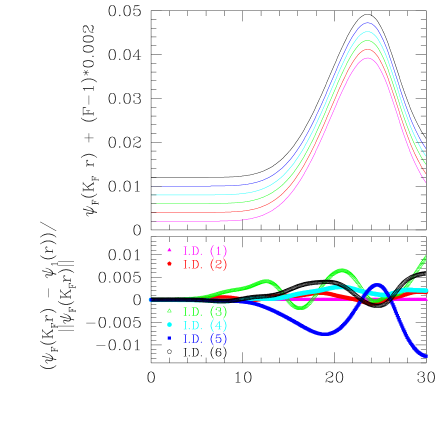
Figure 5: In the top pane we show the spatial profiles (in the region of self-similarity) of the scalar field $\psi$ for different families of initial data, but for fixed angular momentum parameter $l=9$. In particular we show the solutions $\psi_{F}$ calculated from initial data types $F={1,...,6}$ (see Table 2) at times when $\psi_{F}$ reaches maximum amplitude. Each solution is shifted by an amount proportional to its family number for better visualization, with $F=1$ the bottom curve, and $F=6$ the top. The $r$ coordinate is rescaled for each family by a constant factor $K_{F}$, which is family dependent, in such a way that the difference with respect to the profile obtained for the initial data labeled with $F=1$ (for which we consider $K_{1}=1$) is minimized. In the bottom pane we show the differences between the rescaled profiles for $F=2,...,6$ and the profile for $F=1$, divided by the $\ell_{2}$ norm of the solution. The maximum relative difference is of the order of a few percent, providing strong evidence that the critical solution is universal.

Empirically, we have also found that, as we increase $l$ within a family of initial data, although $\Delta_{l}\to 0$ and $T^{\star}_{l}\to 0$, the product $T^{\star}_{l}\Delta_{l}$ appears to asymptote to a finite value. Note that ostensibly this product is family dependent (see Fig. 6), but again that all DSS type-II critical solutions are universal only up to a global scale transformation $(r,t)\to(kr,kt)$, with $k$ an arbitrary positive constant. Choosing $k=k(l)$ for each of the families so that $\max_{r}\left\{2M(t,r)/r\right\}$ is attained at some fiducial radius $r_{0}$, and considering the case $l=10$, we find that the normalized asymptotic oscillation frequency, $f_{0}$, defined by

$$f_{0}=r_{0}/(T^{\star}\Delta)=4.35\pm 0.01$$ (38)

agrees for all families to better than 1%. Again, the quoted uncertainty is estimated from the variation of $f_{0}$ across the different families of initial data. We note that for $l=10$ the near-critical solution stays at a near-constant radial position; our spatial resolution is insufficient to resolve the small changes associated with the extremely small value of $\Delta_{l}$. The radial location of $\max_{r}\left\{2M(t,r)/r\right\}$ in this regime is the value of $r_{0}$ that we have used in (38).

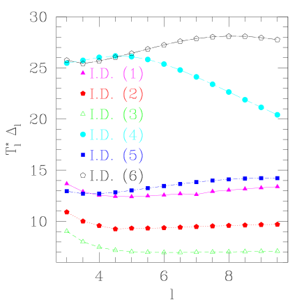
Figure 6: $T^{\star}_{l}\Delta_{l}$ as a function of $l$. The fact that these products remain finite as $T^{\star}_{l}\to\infty$ and $\Delta_{l}\to 0$ is evidence that the critical solutions tend to a periodic solution in the limit $l\to\infty$.

We also note that the observation that $f_{0}$ is apparently well defined and unique (up to the usual rescalings associated with type-II critical solutions), is consistent with the empirical observation that as $l$ increases, the critical solution becomes ever closer to a periodic solution. In particular, for a periodic solution we have $\Delta\to 0$, and then

$$T_{n}-T^{\star} = \left(T_{0}-T^{\star}\right)e^{n\Delta}\approx(T_{0}-T^{\star})\left(1+n\Delta\right)$$ (39)

$$\approx -\left(T^{\star}\Delta\right)n-T^{\star},$$

where $T_{0}$ represents the loosely defined time demarking the onset of the critical regime (and whose precise value is clearly irrelevant in the limit $T^{\star}\to\infty$) which implies that the maximal value is attained at times $T_{n}$:

$$T_{n}=-\left(T^{\star}\Delta\right)n.$$ (40)

As shown in Figs. 7 and 8, from our calculations for $l=10$, we cannot ascertain whether the solution is discretely self-similar with $\Delta_{l}$ very small ($<0.0002$), or periodic with period $\tau=T^{\star}\Delta$.

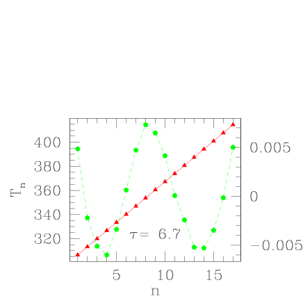
Figure 7: Fit of the times $T_{n}$ at which $\max_{r}\left\{2M(t,r)/r\right\}$ reaches its maximum in time (triangles, left scale) assuming a periodic ansatz. Initial data type $F=1$ was used with angular momentum parameter $l=10$. We also plot the residuals of each data point with respect to the best fit (pentagons, right scale).

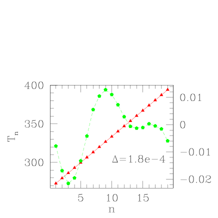
Figure 8: Fit of the times $T_{n}$ at which $\max_{r}\left\{2M(t,r)/r\right\}$ reaches its maximum in time (triangles, left scale) assuming a self-similar ansatz. As in the previous plot, initial data type $F=1$ was used with angular momentum parameter $l=10$. Again, we also plot the residuals of each data point with respect to the best fit (pentagons, right scale). Notice that the errors in the fit are of the same order as the errors in the fit that assumes periodicity (Fig. 7), indicating that from our numerical results we are unable to distinguish between the two types of solutions for $l\geq 10$.

Naively at least, we expect that for $l>10$, distinguishing between discrete self-similarity and periodicity would become even more difficult. However, it is worth noting that for $l=20$ we have not yet seen evidence for (almost)-periodicity, with period $T^{\star}\Delta$, but have instead seen a more complicated structure near criticality that is not yet understood.

IV Conclusions

In this paper, we have discussed the results for a model that incorporates some of the effects of angular momentum in the context of critical gravitational collapse. A new family of spherically-symmetric critical solutions, (black hole threshold solutions) labelled by an angular momentum parameter, $l$, has been found. These solutions have similar properties to those for the $l=0$ case originally studied in Choptuik:jv : specifically, the solutions exhibit discrete self-similarity, and have scaling laws for the values of dimensionful quantities in evolutions close to criticality. We have calculated the $l$-dependence of the echoing exponents $\Delta_{l}$, and the mass-scaling exponents $\gamma_{l}$, finding that both decrease rapidly with increasing $l$, (at least up to $l\approx 10$). Moreover, we have argued that as $l$ increases, the critical solution approaches a periodic evolution.

Together with the results of hlcp , our findings suggest that certain models of collapse may generically admit countable infinities of critical solutions, each member of which can be characterized by distinct near-origin regularity conditions (such as (24-28)) that are preserved by dynamical evolution.

As we explained in the introduction, we expect that $\gamma_{l}=1/\lambda_{l}$ where $\lambda_{l}$ is the Lyapunov exponent associated with the single unstable mode of the critical solution for angular momentum parameter $l$. Therefore since $\gamma_{l}\rightarrow 0$ with increasing $l$, we apparently have $\lambda_{l}\rightarrow\infty$. This has the interpretation of increased stability of the critical solution for increasing $l$, i.e. the period of time that a solution can remain close to criticality (for a fixed amount of fine tuning) increases with $l$. We believe that this can be interpreted as an effect of the angular momentum barrier which (partially) stabilizes the collapse to black hole formation.

Appendix A

We wish to show that the stress energy tensor ${\mathcal{T}}^{(l)a}{}_{b}=\sum_{m}{T^{(lm)}}^{a}{}_{b}$ is independent of $\theta$ and $\phi$, where ${T^{(lm)}}^{a}{}_{b}$ is the stress energy tensor associated with the solution $\psi^{(l)}(t,r)Q_{lm}(\theta,\phi)$, with the same function $\psi^{(l)}(t,r)$, for each value of $m$. For the scalar field, the tensor $T_{ab}$ can be written in terms of the solutions to the wave equation, $\Psi$, as

$$T^{a}{}_{b}=g^{ac}\Psi_{,c}\Psi_{b}-{1\over 2}\delta^{a}{}_{b}g^{dc}\Psi_{,c}\Psi_{d}\,,$$ (41)

and if

$$\sum_{m}M^{a}{}_{b} = g^{ac}{(\psi^{(l)}(t,r)Q_{lm}(\theta,\phi))}_{,c}$$ (42)

$$\times{(\psi^{(l)}(t,r)Q_{lm}(\theta,\phi))}_{,b}$$

is independent of $\theta,~{}\phi$, then so is ${\mathcal{T}}^{(l)a}{}_{b}$.

Using the definition of the $Q_{lm}$ this can be written in terms of the $Y_{lm}$ as

$$\sum_{m}M^{a}{}_{b} = g^{ac}{(\psi^{(l)}(t,r)Y^{*}_{lm}(\theta,\phi))}_{,c}$$ (43)

$$\times{(\psi^{(l)}(t,r)Y_{lm}(\theta,\phi))}_{,b}.$$

We can write this in terms of the Green’s function

$$P(\theta,\phi,\theta^{\prime},\phi^{\prime})=\sum_{m}Y^{*}_{lm}(\theta,\phi)Y_{lm}(\theta^{\prime},\phi^{\prime})$$ (44)

in the limit as $\theta^{\prime}\rightarrow\theta$ and $\phi^{\prime}\rightarrow\phi$.

In bra-ket notation, this is just the operator

$$P=\sum_{m}\left|\left.lm\right\rangle\right.\left\langle\left.lm\right|\right.$$ (45)

which commutes with all of the angular momentum operators.

$$[L_{z},P] = \sum_{m}[L_{z},\left|\left.lm\right\rangle\right.\left\langle\left.lm\right|\right.]$$ (46)

$$= \sum_{m}(m\left|\left.lm\right\rangle\right.\left\langle\left.lm\right|\right.-\left|\left.lm\right\rangle\right.\left\langle\left.lm\right|\right.m)$$

$$= 0,$$

$$[L_{x}+iL_{y},P] = \sum_{m}\left(\sqrt{l(l+1)-m^{2}-m}\left|\left.lm+1\right\rangle\right.\left\langle\left.lm\right|\right.\right.$$ (47)

$$\left.-\left|\left.lm\right\rangle\right.\left((L_{x}-iL_{y})\left|\left.lm\right\rangle\right.\right)^{\dagger}\right)$$

$$= \sum_{m}\left(\sqrt{l(l+1)-m^{2}-m}\left|\left.lm+1\right\rangle\right.\left\langle\left.lm\right|\right.\right.$$

$$\left.-\sqrt{l(l+1)-m^{2}+m}\left|\left.lm\right\rangle\right.\left\langle\left.lm-1\right|\right.\right)$$

$$= 0.$$

Thus $\sum_{m}Y^{*}_{lm}(\theta,\phi)Y_{lm}(\theta^{\prime},\phi^{\prime})$ must be a function of the only rotation invariant function of $\theta,\phi,\theta^{\prime},\phi^{\prime}$, which is the angle $\Theta$ defined by

$$\cos(\Theta)=\cos(\theta)\cos(\theta^{\prime})+\sin(\theta)\sin(\theta^{\prime})\cos(\phi-\phi^{\prime}).$$ (48)

$\Theta$ is the angle between the two unit vectors with directions $\theta,\phi$ and $\theta^{\prime},\phi^{\prime}$ respectively. Since $P$ depends only on $\Theta$ we can choose $\theta=0$ to evaluate it, which gives

$$P(\theta,\phi,\theta^{\prime},\phi^{\prime}) = \sum_{m}Y^{*}_{lm}(\theta,\phi)Y_{lm}(\theta^{\prime},\phi^{\prime})$$ (49)

$$= Y^{*}_{l0}(0,0)Y_{l0}(\Theta,0)$$

$$= {2l+1\over 4\pi}P_{l}(\cos(\Theta)).$$

The various components of the tensor $M$ are of three types: ones with no derivatives with respect to $\theta$ or $\phi$ (eg $M_{tt}$), those with one derivative, (for example $M_{t\theta}$) and those with two (eg, $M_{\theta\theta}$). The ones with no derivatives will be functions of $\lim_{\theta^{\prime},\phi^{\prime}\rightarrow\theta,\phi}P=\sqrt{(2l+1)/(4\pi)}\,P_{l}(1)$ which is clearly independent of $\theta,\phi$. The terms with one $\theta,\phi$ derivative will be functions of

$$\lim_{\Theta\rightarrow 0}\partial_{\theta,\phi}P_{l}(\cos(\Theta)) = \lim_{\Theta\rightarrow 0}P_{l}^{\prime}\{\sin(\Theta),\sin^{2}(\theta)\sin(\phi-\phi^{\prime})\}$$ (50)

$$= 0,$$

and similarly the term

$$M_{\theta\phi} \propto \lim_{\Theta\rightarrow 0}\partial_{\theta}\partial_{\phi^{\prime}}P_{l}(\cos(\Theta))\propto\lim_{\phi\rightarrow\phi^{\prime}}\sin(\phi-\phi^{\prime})$$ (51)

$$= 0.$$

Thus the only two terms remaining are

$$M_{\theta\theta} \propto \lim_{\theta\rightarrow\theta^{\prime}}\partial_{\theta}\partial_{\theta^{\prime}}P_{l}(\cos(\theta-\theta^{\prime}))$$ (52)

$$= P_{l}^{\prime}(\cos(0))(-\cos(0))(-1)$$

$$= P_{l}^{\prime}(1)\,,$$

$$M_{\phi\phi^{\prime}} \propto P_{l}^{\prime}(1)\sin(\theta)^{2}\,.$$ (53)

Thus the non-zero components of the tensor $M$ are $M_{tt},~{}M_{tr},~{}M_{rr},~{}M_{\phi\phi}=\sin^{2}(\theta)M_{\theta\theta}$, with only $M_{\phi\phi}$ having $\theta$ dependence. Thus, $M^{a}{}_{b}$ will be independent of $\theta,\phi$ and therefore so will ${\mathcal{T}}^{(l)a}{}_{b}$, as required.

In addition, from the equations of motion for the individual fields $\Psi_{lm}$, each of the energy momentum tensors for given $l,m$ is conserved in the overall spherically symmetric spacetime. Thus, so is their sum over $m$ for any given $l$, and we have

$${\mathcal{T}}^{(l)a}{}_{b;a}=0\,.$$ (54)

References

- (1) C. Gundlach, Living Rev. Rel. 2, 4 (1999) [arXiv:gr-qc/0001046].
- (2) C. Gundlach, Phys. Rept. 376, 339 (2003) [arXiv:gr-qc/0210101].
- (3) A. M. Abrahams and C. R. Evans, Phys. Rev. Lett. 70, 2980 (1993).
- (4) S. L. Liebling, Phys. Rev. D66, 041703, (2002) [arXiv:gr-qc/0202093].
- (5) S. Hod and T. Piran, Phys. Rev. D55, 440 (1997) [arXiv:gr-qc/9606087].
- (6) C. Gundlach, Phys. Rev. D55, 695 (1997) [arXiv:gr-qc/9604019].
- (7) M. W. Choptuik, E. W. Hirschmann, S. L. Liebling and F. Pretorius, Phys. Rev. D68, 044007, (2003) [arXiv:gr-qc/0305003].
- (8) D. Garfinkle, C. Gundlach and J. M. Martin-Garcia, Phys. Rev. D59, 104012, (1999) [arXiv:gr-qc/9811004].
- (9) C. Gundlach, Phys. Rev. D57, 7080, (1998) [arXiv:gr-qc/9711079].
- (10) C. Gundlach, Phys. Rev. D65, 084021, (2002) [arXiv:gr-qc/9906124].
- (11) M. W. Choptuik, E. W. Hirschmann, S. L. Liebling and F. Pretorius, Phys. Rev. Lett. 93, 131101 (2004) [arXiv:gr-qc/0405101].
- (12) G. Rein, A. D. Rendall and J. Schaeffer, Phys. Rev. D58, 044007, (1998) [arXiv:gr-qc/9804040].
- (13) I. Olabarrieta and M. W. Choptuik, Phys. Rev. D65, 024007, (2002) [arXiv:gr-qc/0107076].
- (14) J. F. Ventrella and M. W. Choptuik, Phys. Rev. D68, 044020 (2003) [arXiv:gr-qc/0304007].
-
(15)
R. L. Marsa and M. W. Choptuik,
http://laplace.phas.ubc.ca/users_guide/users_guide.html (1995). - (16) H. Kreiss and J. Oliger, Global Atmospheric Research Programme, Publications Series No. 10. (1973).
- (17) M. W. Choptuik, Phys. Rev. Lett. 70, 9, (1993).
- (18) S. L. Liebling, Phys. Rev. D60, 061502, (1999) [arXiv:gr-qc/9904077].
- (19) S. Husa, C. Lechner, M. Purrer, J. Thornburg and P. C. Aichelburg, Phys. Rev. D62, 104007, (2000) [arXiv:gr-qc/0002067].
- (20) D. Garfinkle and G. C. Duncan, Phys. Rev. D58, 064024, (1998) [arXiv:gr-qc/9802061].