Single hole and vortex excitations in the doped Rokhsar-Kivelson quantum dimer model on the triangular lattice

Abstract

We consider the doped Rokhsar-Kivelson quantum dimer model on the triangular lattice with one mobile hole (monomer) at the Rokhsar-Kivelson point. The motion of the hole is described by two branches of excitations: the hole may either move with or without a trapped Z₂ vortex (vison). We perform a study of the hole dispersion in the limit where the hole hopping amplitude is much smaller than the interdimer interaction. In this limit, the hole without vison moves freely and has a tight-binding spectrum. On the other hand, the hole with a trapped vison is strongly constrained due to interference effects and can only move via higher-order virtual processes.

I Introduction

Quantum dimer models in two dimensions are an active field of research due to their possible relevance to high-temperature superconductivityRK87 ; RK88 ; kivelson89 and to frustrated magnetism,Read-Sachdev in the framework of the resonating-valence-bond (RVB) construction.anderson87 It was, however, realized that the RVB liquid state of the original Rokhsar-Kivelson (RK) dimer model on the square lattice is criticalfisher6163 and does not provide a stable phase. A search for a liquid with topological orderwen91 continued with quantum dimer models on nonbipartite lattices,ms01_2 in particular on the triangular lattice. At a special value of the coupling constants (the RK point), the RK dimer model on the triangular lattice is proven to have exponentially decaying correlations,ms01 ; Ioselevich and a gapped excitation spectrum is found numerically.dima04 Furthermore, there is now convincing numerical evidence that this gapped liquid phase is stable and extends within a finite parameter range.arnaud

In the RVB scenario of high-temperature superconductivity, the superconductivity emerges upon doping a liquid of singlet bonds with charge carriers.anderson87 ; lee06 ; pvrvb ; foot Very early it was therefore proposed to study quantum dimer models containing monomersRK88 ; kivelson89 (see Refs. syl04, ; poilblanc06, ; castelnovo07, ; arnaudPhaseSep, ; fradkin07, for more recent studies). When analyzing a hole in the background of dimer or spin liquids, one should take into account vortexlike excitations inherent in topological liquids.kivelson89 ; RC89 These topological excitations were dubbed visons in the context of the corresponding Z₂ gauge theory.SF There is now evidence that visons constitute the gapped excitations of the undoped triangular-lattice quantum dimer liquid.dima04 ; arnaud It is known that visons can bind to holes and change their statistics.kivelson89 ; RC89

In this work, we study the properties of a single-hole excitation in the case of a doped triangular-lattice quantum dimer model at the RK point and illustrate the hole-vison binding. We find two branches of excitations: one for the hole itself and the other for a hole-vison bound state. The energy-momentum dispersion for both branches of excitations is computed in the perturbative regime of small hole hopping. The combined effects of lattice frustration and Z₂ flux lead to a quadruply degenerate vison-hole branch and reduced bandwidth. These results may have interesting implications for RVB physics.

This paper is organized in the following way. In Sec. II, we introduce the model and show the existence of two branches of excitations. In Sec. III, we calculate perturbatively the dispersion of the non-vison branch of the hole excitation. In Sec. IV, the dispersion of the vison branch is calculated. Finally, in Sec. V, we summarize and discuss our results.

II Doped dimer model, topological sectors, and two branches of excitations

We consider the quantum dimer model on the triangular lattice doped with mobile holes. We choose the simplest form of the hole-hopping term which involves rearrangement of one dimer. The Hamiltonian reads

$$H_{RK+hole}=$$

$$\sum_{\begin{minipage}{9.79836pt} \begin{center} \begin{picture}(30.0,17.0)\put(0.0,0.0){\circle*{4.0}} \put(20.0,0.0){\circle*{4.0}} \put(10.0,17.3){\circle*{4.0}} \put(30.0,17.3){\circle*{4.0}} \put(0.0,0.0){\line(1,0){20.0}} \put(10.0,17.3){\line(1,0){20.0}} \qbezier(0.0,0.0)(5.0,8.65)(10.0,17.3)\qbezier(20.0,0.0)(25.0,8.65)(30.0,17.3)\end{picture} \end{center} \end{minipage}}\left[-t\left(|\begin{minipage}{13.99765pt} \begin{center} \begin{picture}(30.0,17.0)\put(0.0,0.0){\circle*{4.0}} \put(20.0,0.0){\circle*{4.0}} \put(10.0,17.3){\circle*{4.0}} \put(30.0,17.3){\circle*{4.0}} \qbezier(0.0,0.0)(5.0,8.65)(10.0,17.3)\qbezier(20.0,0.0)(25.0,8.65)(30.0,17.3)\end{picture} \end{center} \end{minipage}\rangle\langle\begin{minipage}{13.99765pt} \begin{center} \begin{picture}(30.0,17.0)\put(0.0,0.0){\circle*{4.0}} \put(20.0,0.0){\circle*{4.0}} \put(10.0,17.3){\circle*{4.0}} \put(30.0,17.3){\circle*{4.0}} \put(0.0,0.0){\line(1,0){20.0}} \put(10.0,17.3){\line(1,0){20.0}} \end{picture} \end{center} \end{minipage}|+\mathrm{h.c.}\right)+v\left(|\begin{minipage}{13.99765pt} \begin{center} \begin{picture}(30.0,17.0)\put(0.0,0.0){\circle*{4.0}} \put(20.0,0.0){\circle*{4.0}} \put(10.0,17.3){\circle*{4.0}} \put(30.0,17.3){\circle*{4.0}} \put(0.0,0.0){\line(1,0){20.0}} \put(10.0,17.3){\line(1,0){20.0}} \end{picture} \end{center} \end{minipage}\rangle\langle\begin{minipage}{13.99765pt} \begin{center} \begin{picture}(30.0,17.0)\put(0.0,0.0){\circle*{4.0}} \put(20.0,0.0){\circle*{4.0}} \put(10.0,17.3){\circle*{4.0}} \put(30.0,17.3){\circle*{4.0}} \put(0.0,0.0){\line(1,0){20.0}} \put(10.0,17.3){\line(1,0){20.0}} \end{picture} \end{center} \end{minipage}|+|\begin{minipage}{13.99765pt} \begin{center} \begin{picture}(30.0,17.0)\put(0.0,0.0){\circle*{4.0}} \put(20.0,0.0){\circle*{4.0}} \put(10.0,17.3){\circle*{4.0}} \put(30.0,17.3){\circle*{4.0}} \qbezier(0.0,0.0)(5.0,8.65)(10.0,17.3)\qbezier(20.0,0.0)(25.0,8.65)(30.0,17.3)\end{picture} \end{center} \end{minipage}\rangle\langle\begin{minipage}{13.99765pt} \begin{center} \begin{picture}(30.0,17.0)\put(0.0,0.0){\circle*{4.0}} \put(20.0,0.0){\circle*{4.0}} \put(10.0,17.3){\circle*{4.0}} \put(30.0,17.3){\circle*{4.0}} \qbezier(0.0,0.0)(5.0,8.65)(10.0,17.3)\qbezier(20.0,0.0)(25.0,8.65)(30.0,17.3)\end{picture} \end{center} \end{minipage}|\right)\right]$$

$$+\sum_{\begin{minipage}{9.79836pt} \begin{center} \begin{picture}(30.0,17.0) \put(0.0,0.0){\circle*{4.0}} \put(20.0,0.0){\circle*{4.0}} \put(10.0,17.3){\circle*{4.0}} \put(0.0,0.0){\line(1,0){20.0}} \qbezier(0.0,0.0)(5.0,8.65)(10.0,17.3)\qbezier(20.0,0.0)(5.0,25.95)(10.0,17.3)\end{picture} \end{center} \end{minipage}}\left[-s\left(|\begin{minipage}{13.99765pt} \begin{center} \begin{picture}(30.0,17.0) \put(0.0,0.0){\circle*{4.0}} \put(20.0,0.0){\circle*{4.0}} \put(10.0,17.3){\circle*{4.0}} \put(0.0,0.0){\line(1,0){20.0}} \end{picture} \end{center} \end{minipage}\rangle\langle\begin{minipage}{13.99765pt} \begin{center} \begin{picture}(30.0,17.0) \put(0.0,0.0){\circle*{4.0}} \put(20.0,0.0){\circle*{4.0}} \put(10.0,17.3){\circle*{4.0}} \qbezier(20.0,0.0)(5.0,25.95)(10.0,17.3)\end{picture} \end{center} \end{minipage}|+\mathrm{h.c.}\right)+2u|\begin{minipage}{13.99765pt} \begin{center} \begin{picture}(30.0,17.0) \put(0.0,0.0){\circle*{4.0}} \put(20.0,0.0){\circle*{4.0}} \put(10.0,17.3){\circle*{4.0}} \qbezier(0.0,0.0)(5.0,8.65)(10.0,17.3)\end{picture} \end{center} \end{minipage}\rangle\langle\begin{minipage}{13.99765pt} \begin{center} \begin{picture}(30.0,17.0) \put(0.0,0.0){\circle*{4.0}} \put(20.0,0.0){\circle*{4.0}} \put(10.0,17.3){\circle*{4.0}} \qbezier(0.0,0.0)(5.0,8.65)(10.0,17.3)\end{picture} \end{center} \end{minipage}|\right]$$

$$=H_{RK}+H_{s}\;,$$ (1)

where the first sum is performed over all three orientations of rhombi and the second sum is over both up and down triangles and over all three possible positions of the hole on the triangle.

We consider the model [Eq. (II)] at the RK point, $t=v=1$, in the sector with a single hole. At $s=u\geq 0$, the Hamiltonian has the usual “supersymmetric” properties of the RK point: its ground state is exactly known and given by the equal-amplitude superposition of all possible states,RK88 and the quantum mechanics can be mapped onto a classical stochastic dynamics in imaginary time.henley04 We further consider the hole term $H_{s}$ as a perturbation in $s\ll 1$, $u\ll 1$. To simplify the formulae, we assume $u=s\geq 0$, but our results are trivially extendable to $u\neq s$.

In the unperturbed Hamiltonian $H_{RK}$, the position of the hole $x$ is a static parameter. We consider the hole on the infinite lattice (or, equivalently, on a large finite lattice far from the boundary). In such a setup there are two degenerate ground states of $H_{RK}$ for each hole position. They correspond to two disconnected (topological) sectors $\mathcal{H}^{\pm}(x)$ of the Hilbert space, characterized by the values $\pm 1$ of the vison operator

$$V(x)=(-1)^{\text{No. of dimers intersecting $\Gamma_{x}$}},$$ (2)

for some contour $\Gamma_{x}$ connecting the hole position $x$ to infinity (in a finite system to the boundary). kivelson89 ; RC89 The corresponding ground states are given by the sums over all dimer coverings in the respective topological sector and are denoted as $\psi_{0}^{\pm}(x)$. Note that while the labeling $\pm$ of the two sectors $\mathcal{H}^{\pm}(x)$ depends on the choice of the contour $\Gamma_{x}$, the sectors themselves do not. Changing the contour $\Gamma_{x}$ amounts to possible interchanges $\mathcal{H}^{+}(x)\leftrightarrow\mathcal{H}^{-}(x)$ and, therefore, $\psi_{0}^{+}(x)\leftrightarrow\psi_{0}^{-}(x)$. This ambiguity reflects the Z₂ degree of freedom in labeling the topological sectors, and it will play an important role in the motion of the hole with a trapped vison. Technically, this Z₂ gauge may be fixed by specifying (arbitrarily), for each $x$, a reference dimer covering which belongs to $\mathcal{H}^{+}(x)$.

The two topological sectors $\mathcal{H}^{\pm}(x)$ differ by the parity of the dimer intersection at infinity and hence are indistinguishable by any local operator (since all correlation functions are short-ranged in the RK model on the triangular lattice ms01 ; Ioselevich ). Therefore, for excitations obtained from the ground states by local operators (in the vicinity of $x$), one can establish a one-to-one linear mapping between the states in $\mathcal{H}^{+}(x)$ and in $\mathcal{H}^{-}(x)$. Taking odd and even combinations of the corresponding states $\psi^{+}(x)\pm\psi^{-}(x)$, we obtain the decomposition of the Hilbert space into even and odd sectors $\mathcal{H}^{e,o}(x)$. Those even and odd sectors correspond to the non-vison and vison sectors of excitations, respectively, introduced in Ref. dima04, .

The key observation for our discussion is that the Hamiltonian [Eq. (II)] preserves the decomposition into $\mathcal{H}^{e,o}(x)$ at every point $x$. While it is obviously true for $H_{RK}$ and the potential part of $H_{s}$, one can also easily check that the hopping part of $H_{s}$ does not have matrix elements between $\mathcal{H}^{e}(x)$ and $\mathcal{H}^{o}(x^{\prime})$ for neighboring sites $x$ and $x^{\prime}$. Hence, the excitations of the moving hole can also be classified into two branches: the non-vison branch [contained in $\oplus_{x}\mathcal{H}^{e}(x)$] and the vison branch [contained in $\oplus_{x}\mathcal{H}^{o}(x)$]. This splitting into even (non-vison) and odd (vison) branches is a generic feature of any perturbative mixing of topological sectors in quantum dimer models.

III Non-vison branch

The energy spectrum of the non-vison branch can be easily calculated to first order in the perturbative expansion in $H_{s}$. We can fix the phases of all RK ground states $\psi^{e}_{0}(x)=\psi^{+}_{0}(x)+\psi^{-}_{0}(x)$ by taking the linear combination of all dimer coverings with the amplitude one (up to normalization). Then, the problem of the moving hole maps onto the tight-binding model with the hopping amplitude

$$t_{1}=-\langle\psi^{e}_{0}(x)|H_{s}|\psi^{e}_{0}(x^{\prime})\rangle$$ (3)

for nearest-neighbor $x$ and $x^{\prime}$ (here and in the following we always assume normalized states). This amplitude may be converted into an expectation value in the RK model with a static hole,

$$t_{1}=2s\langle\psi_{0}(x)|\begin{minipage}{13.99765pt} \begin{center} \begin{picture}(30.0,17.0) \put(0.0,0.0){\circle*{4.0}} \put(20.0,0.0){\circle*{4.0}} \put(10.0,17.3){\circle*{4.0}} \put(0.0,0.0){\line(1,0){20.0}} \end{picture} \end{center} \end{minipage}\rangle\langle\begin{minipage}{13.99765pt} \begin{center} \begin{picture}(30.0,17.0) \put(0.0,0.0){\circle*{4.0}} \put(20.0,0.0){\circle*{4.0}} \put(10.0,17.3){\circle*{4.0}} \put(0.0,0.0){\line(1,0){20.0}} \end{picture} \end{center} \end{minipage}|\psi_{0}(x)\rangle=2s\frac{N_{3}}{N_{1}}\,,$$ (4)

where $N_{1}$ and $N_{3}$ are the numbers of dimer coverings with one site and one three-site triangle removed, respectively. The ratio $N_{3}/N_{1}$ is well defined in the limit of the infinite system and can be computed numerically with a suitable method. We have calculated this coefficient with a Monte Carlo simulation similar to that in Refs. Ioselevich, and dima04, (using clusters of toroidal geometry with up to 17$\times$17 sites), with the result $N_{3}/N_{1}=0.229\pm 0.001$.

Taking into account the potential term in $H_{s}$ and performing the Fourier transformation in $x$, the dispersion of the hole without a vison takes the form

$$E_{\bf k}=-2t_{1}(\cos k_{1}+\cos k_{2}+\cos k_{3}-3)\,,$$ (5)

where $k_{1}$, $k_{2}$, and $k_{3}$ are the projections of the vector ${\bf k}$ on the three lattice directions (with $k_{1}+k_{2}+k_{3}=0$).

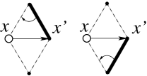
Figure 1: These two types of hopping processes set opposite correspondences between the sectors $\mathcal{H}^{\pm}(x)$ and $\mathcal{H}^{\pm}(x^{\prime})$, and therefore cancel each other in Eq. (6).

IV Vison branch

The hopping of a hole with a trapped vison is more complicated. The phases of the odd-sector ground states, $\psi^{o}_{0}(x)=\psi_{0}^{+}(x)-\psi_{0}^{-}(x)$, cannot be synchronized invariantly for all $x$, which reflects the frustration of the vison motion. dima04 The freedom of the Z₂ gauge [the contours $\Gamma_{x}$ in Eq. (2) or, equivalently, the reference dimer configuration for each $x$] corresponds to the choice of the overall sign for the states in ${\mathcal{H}}^{o}(x)$.

Regardless of the chosen Z₂ gauge, the hopping amplitude vanishes to first order,

$$\langle\psi^{o}_{0}(x)|H_{s}|\psi^{o}_{0}(x^{\prime})\rangle=0$$ (6)

for nearest-neighbors $x$ and $x^{\prime}$. This can be seen as the cancellation of the two types of hopping processes from $x$ to $x^{\prime}$, corresponding to two possible dimer flips (Fig. 1). Each of those dimer flips maps each of $\mathcal{H}^{\pm}(x)$ into one of $\mathcal{H}^{\pm}(x^{\prime})$. The change in topological sector depends on the chosen gauge, but the correspondence between the two sectors $\mathcal{H}^{\pm}(x)$ and the two sectors $\mathcal{H}^{\pm}(x^{\prime})$ is opposite for the two types of flips. hugo_thesis As a result, the corresponding processes connecting two ground states $\psi^{o}_{0}(x)$ and $\psi^{o}_{0}(x^{\prime})$ exactly cancel each other.

A nontrivial hopping appears only to higher order in perturbation theory for some trajectories. The second-order hopping amplitude

$$t_{2}=\sum_{x^{\prime},n\neq 0}\frac{1}{E_{n}}\langle\psi^{o}_{0}(x)|H_{s}|\psi^{o}_{n}(x^{\prime})\rangle\langle\psi^{o}_{n}(x^{\prime})|H_{s}|\psi^{o}_{0}(x^{\prime\prime})\rangle$$ (7)

involves excitations $\psi^{o}_{n}(x^{\prime})$ of $H_{RK}$ with energies $E_{n}$.

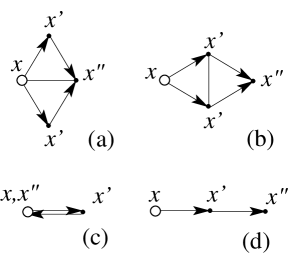
Figure 2: The two trajectories of the hole exactly cancel each other in the second order of the perturbation theory [Eq. (7)] for (a) nearest-neighbor and (b) next-nearest-neighbor hoppings. The nonvanishing second-order terms are (c) on-site and (d) next-next-nearest-neighbor hoppings.

Similarly to the cancellation of the nearest-neighbor hopping amplitude to first order in perturbation, one can show the cancellation to second order of the hopping processes $x\to x^{\prime}\to x^{\prime\prime}$ connecting nearest-neighbor and next-nearest-neighbor sites [processes (a) and (b) in Fig. 2]. One can verify that, in those cases, processes symmetric with respect to the line $xx^{\prime\prime}$ exactly cancel each other.

The only nontrivial hopping in the second order occurs for trajectories $x\to x^{\prime}\to x^{\prime\prime}$ involving two links along the same direction [i.e., for the on-site energy correction and for the next-next-nearest-neighbor hopping, processes (c) and (d) in Fig. 2]. The corresponding next-next-nearest-neighbor hopping amplitude [Fig. 2(d)] to second order in perturbation [Eq. (7)] may be expressed via dynamic correlation functions in the RK model with a static hole at position $x^{\prime}$,

$$t_{2} = \int_{0}^{\infty}dt\langle\psi^{o}_{0}(x)|H_{s}e^{-H_{RK}t}H_{s}|\psi^{o}_{0}(x^{\prime\prime})\rangle$$ (8)

$$= s^{2}\int_{0}^{\infty}dt\,I(t)\,,$$

where

$$I(t)=\langle\psi_{0}(x^{\prime})|P_{xx^{\prime}}e^{-H_{RK}t}P_{x^{\prime}x^{\prime\prime}}|\psi_{0}(x^{\prime})\rangle$$ (9)

and

$$P_{xx^{\prime}} = |\begin{minipage}{13.99765pt} \begin{center} \begin{picture}(30.0,17.0) \put(0.0,0.0){\circle*{4.0}} \put(20.0,0.0){\circle*{4.0}} \put(10.0,17.3){\circle*{4.0}} \qbezier(0.0,0.0)(5.0,8.65)(10.0,17.3)\end{picture} \end{center} \end{minipage}\rangle\langle\begin{minipage}{13.99765pt} \begin{center} \begin{picture}(30.0,17.0) \put(0.0,0.0){\circle*{4.0}} \put(20.0,0.0){\circle*{4.0}} \put(10.0,17.3){\circle*{4.0}} \qbezier(0.0,0.0)(5.0,8.65)(10.0,17.3)\end{picture} \end{center} \end{minipage}|-|\begin{minipage}{13.99765pt} \begin{center} \begin{picture}(30.0,17.0) \put(20.0,0.0){\circle*{4.0}} \put(10.0,17.3){\circle*{4.0}} \put(30.0,17.3){\circle*{4.0}} \qbezier(20.0,0.0)(6.0,25.95)(10.0,17.3)\end{picture} \end{center} \end{minipage}\rangle\langle\begin{minipage}{13.99765pt} \begin{center} \begin{picture}(30.0,17.0) \put(20.0,0.0){\circle*{4.0}} \put(10.0,17.3){\circle*{4.0}} \put(30.0,17.3){\circle*{4.0}} \qbezier(20.0,0.0)(6.0,25.95)(10.0,17.3)\end{picture} \end{center} \end{minipage}|$$

$$P_{x^{\prime}x^{\prime\prime}} = |\begin{minipage}{13.99765pt} \begin{center} \begin{picture}(30.0,17.0) \put(20.0,0.0){\circle*{4.0}} \put(10.0,17.3){\circle*{4.0}} \put(30.0,17.3){\circle*{4.0}} \qbezier(20.0,0.0)(15.0,-8.65)(30.0,17.3)\end{picture} \end{center} \end{minipage}\rangle\langle\begin{minipage}{13.99765pt} \begin{center} \begin{picture}(30.0,17.0) \put(20.0,0.0){\circle*{4.0}} \put(10.0,17.3){\circle*{4.0}} \put(30.0,17.3){\circle*{4.0}} \qbezier(20.0,0.0)(15.0,-8.65)(30.0,17.3)\end{picture} \end{center} \end{minipage}|-|\begin{minipage}{13.99765pt} \begin{center} \begin{picture}(30.0,17.0) \put(0.0,0.0){\circle*{4.0}} \put(20.0,0.0){\circle*{4.0}} \put(10.0,17.3){\circle*{4.0}} \qbezier(20.0,0.0)(5.0,25.95)(10.0,17.3)\end{picture} \end{center} \end{minipage}\rangle\langle\begin{minipage}{13.99765pt} \begin{center} \begin{picture}(30.0,17.0) \put(0.0,0.0){\circle*{4.0}} \put(20.0,0.0){\circle*{4.0}} \put(10.0,17.3){\circle*{4.0}} \qbezier(20.0,0.0)(5.0,25.95)(10.0,17.3)\end{picture} \end{center} \end{minipage}|\,.$$ (10)

The dynamic correlation function $I(t)$ is well defined in the limit of infinite system size and does not depend on the topological sector in this limit. It may be computed with a classical Monte Carlo method as in Ref. dima04, . Using clusters of toroidal geometry and up to 17$\times$17 sites, we find $\int_{0}^{\infty}dt\;I(t)=-1.51\pm 0.08$ (observe that it is negative).

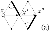
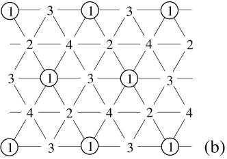
Figure 3: (a) We fix the relative gauge at the next-next-nearest-neighbor sites by relating the reference configurations in $\mathcal{H}^{+}(x)$ and $\mathcal{H}^{+}(x^{\prime\prime})$ via two consecutive dimer flips on opposite sides of the line $xx^{\prime}x^{\prime\prime}$. (b) The four sublattices connected by the hopping of the vison-hole bound state. This composite excitation can only hop by multiples of two lattice periods.

Note that the sign of $t_{2}$ in Eq. (8)] corresponds to a particular relative gauge choice at points $x$ and $x^{\prime\prime}$: the reference dimer coverings at $x$ and $x^{\prime\prime}$ are connected by two dimer flips on opposite sides of the line $xx^{\prime}x^{\prime\prime}$ (Fig. 3). One can show that this local gauge convention for any two sites separated by two lattice periods can be consistently extended to a global gauge on the sublattice of such sites (with the period of this sublattice equals twice that of the original lattice). There are four such sublattices (Fig. 3), and the hole-vison excitation hops on each of them independently, without a possibility to cross over to another sublattice. The resulting dispersion relation is that of the tight-binding model with the doubled lattice constant and the hopping amplitude given by Eq.  (8),

$$E_{\bf k}^{\rm(v)}=-2t_{2}(\cos 2k_{1}+\cos 2k_{2}+\cos 2k_{3})+\varepsilon_{0}\,.$$ (11)

The on-site energy $\varepsilon_{0}$ is equal to that in the non-vison sector in Eq. (5). To leading order in $s$, it is given by $\varepsilon_{0}=6t_{1}$.

The hole-vison excitations with dispersion (11) are quadruply degenerate (by sublattice) for each value of ${\bf k}$ in the Brillouin zone of the doubled lattice. While we have explicitly demonstrated this degeneracy to second order, it can be extended to all orders of perturbation theory. In fact, this degeneracy is determined by the symmetries of the original Hamiltonian [Eq. (II)] in the vison sector and can thus be promoted from a perturbative argument to the exact spectrum. The exact degeneracy can be proven using the translational invariance of the Hamiltonian, together with the symmetry under point inversion (rotation by $\pi$) and time reversal. Physically, this degeneracy can be understood as the cancellation of virtual processes for the flux-carrying excitation on the frustrated triangular lattice.

Finally, let us note that, while our derivation of the vison-hole spectrum was formally done at the RK-point, its form and degeneracy are the same in the whole liquid phase away from the RK point (estimated to extend to the region $0.8\lesssim\frac{v}{t}\leq 1$ in Ref. arnaud, ), provided the hole hopping is small. Only the numerical coefficients in the hopping amplitudes $t_{1}$ and $t_{2}$ get modified in this case. Furthermore, our results equally apply when more than one hole is present in the system as long as the holes are sufficiently far apart and do not interact with each other.

V Summary

In this paper, we have calculated the dispersion of a single mobile hole in the RVB liquid phase of the doped RK quantum dimer model on the triangular lattice. We find two branches of excitations: one for the bare hole and the other for a hole-vison bound state. The effective motion of the hole-vison state is strongly modified by the Z₂ flux associated with the vison. Interference effects due to lattice frustration reduce the bandwidth of this type of excitation and lead to additional degeneracies. These are general properties, which should be observed in any doped Z₂ RVB liquid on frustrated lattices.

In our specific model [Eq. (II)], the energy of a static ($s=0$) vison-hole bound state equals that of a hole without a vison. In other words, the vison does not cost any energy if placed in a hole (while in the bulk, its energy is a finite fraction of $t$, see Ref. dima04, ). In the limit of a small hopping amplitude $s$, the energy of a static excitation is split, with the bandwidth proportional to $s$ for the bare hole and to $s^{2}/t$ for the hole-vison bound state. As a result, the two branches intersect each other, with the minimum of energy (the ground state) corresponding to the hole without a vison. For some ${\bf k}$ in a region close to the boundary of the Brillouin zone, the vison-hole bound state is lower in energy than the bare hole. In a more general quantum dimer model (or in other RVB-type systems), however, one may imagine the situation where the hole-vison bound state constitutes the ground state (in our dimer model, this may be achieved, for example, by adding ring exchange of dimers around a hole). In such a case, the doped holes spontaneously generate visons, which, in turn, may lead to further interesting effects, e.g., the modification of the statistics of holes.RC89 ; kivelson89

- (1) S. A. Kivelson, D. S. Rokhsar, and J. P. Sethna, Phys. Rev. B 35, 8865 (1987).
- (2) D. S. Rokhsar and S. A. Kivelson, Phys. Rev. Lett. 61, 2376 (1988).
- (3) S. A. Kivelson, Phys. Rev. B 39, 259 (1989).
- (4) N. Read and S. Sachdev, Phys. Rev. Lett. 66, 1773 (1991).
- (5) P. W. Anderson, Science 235, 1196 (1987).
- (6) M. E. Fisher, Phys. Rev. 124, 1664 (1961); M. E. Fisher and J. Stephenson, ibid. 132, 1411 (1963).
- (7) X. G. Wen, Phys. Rev. B 40, 7387(R) (1989); 44, 2664 (1991); X. G. Wen and Q. Niu, ibid. 41, 9377 (1990); X. G. Wen, Int. J. Mod. Phys. B 4, 239 (1990).
- (8) R. Moessner and S. L. Sondhi, Phys. Rev. B 63, 224401 (2001).
- (9) R. Moessner and S. L. Sondhi, Phys. Rev. Lett. 86, 1881 (2001); P. Fendley, R. Moessner, and S. L. Sondhi, Phys. Rev. B 66, 214513 (2002).
- (10) A. Ioselevich, D. A. Ivanov, and M. V. Feigelman, Phys. Rev. B 66, 174405 (2002).
- (11) D. A. Ivanov, Phys. Rev. B 70, 94430 (2004).
- (12) A. Ralko, M. Ferrero, F. Becca, D. Ivanov, and F. Mila, Phys. Rev. B 71, 224109 (2005); 74, 134301 (2006); 76, 140404(R) (2007).
- (13) P. Lee, N. Nagaosa, and X.-G. Wen, Rev. Mod. Phys. 78, 17 (2006).
- (14) P. W. Anderson, P. A. Lee, M. Randeria, M. Rice, N. Trivedi, and F. C. Zhang, J. Phys. Condens. Matter 16, R755 (2004).
- (15) N. Read and B. Chakraborty, Phys. Rev. B 40, 7133 (1989).
- (16) D. Poilblanc, F. Alet, F. Becca, A. Ralko, F. Trousselet, and F. Mila, Phys. Rev. B 74, 14437 (2006).
- (17) O. F. Syljuåsen, Phys. Rev. B 71, 020401(R) (2005).
- (18) C. Castelnovo, C. Chamon, Ch. Mudry, and P. Pujol, Ann. Phys. 322, 903 (2007).
- (19) A. Ralko, F. Mila, and D. Poilblanc, Phys. Rev. Lett. 99, 127202 (2007).
- (20) S. Papanikolaou, E. Luijten, and E. Fradkin, Phys. Rev. B 76, 134514 (2007).
- (21) T. Senthil and M. P. A. Fisher, Phys. Rev. B 62, 7850 (2000); 63, 134521 (2001).
- (22) C. L. Henley, J. Phys. Condens. Matter 16, 891 (2004).
- (23) H. Ribeiro, M. S. thesis, Institute of Theoretical Physics, Ecole Polytechnique Fédérale de Lausanne, 2007.
- (24) S. Yunoki and S. Sorella, Phys. Rev. B 74, 014408 (2006).
- (25) M. E. Zhitomirsky, Phys. Rev. B 71, 214413 (2005).
- (26) F. Vernay, A. Ralko, F. Becca, and F. Mila, Phys. Rev. B 74, 054402 (2006).
- (27) While high-temperature superconductors are now believed to be described by a long-range RVB liquid [Ref. pvrvb, ], promising short-range RVB states have been proposed recently for several frustrated spin systems. See, e.g., Refs. ys06, ; mike05, ; francois06, .