Self-similar Radiation from Numerical Rosenau-Hyman Compactons

Abstract

The numerical simulation of compactons, solitary waves with compact support, is characterized by the presence of spurious phenomena, as numerically-induced radiation, which is illustrated here using four numerical methods applied to the Rosenau-Hyman $K(p,p)$ equation. Both forward and backward radiations are emitted from the compacton presenting a self-similar shape which has been illustrated graphically by the proper scaling. A grid refinement study shows that the amplitude of the radiations decreases as the grid size does, confirming its numerical origin. The front velocity and the amplitude of both radiations have been studied as a function of both the compacton and the numerical parameters. The amplitude of the radiations decreases exponentially in time, being characterized by a nearly constant scaling exponent. An ansatz for both the backward and forward radiations corresponding to a self-similar function characterized by the scaling exponent is suggested by the present numerical results.

,

1 Introduction

Compactons are travelling wave solutions with compact support resulting from the balance of both nonlinearity and nonlinear dispersion. Compacton solutions have been first found in a generalized Korteweg-de Vries equation with nonlinear dispersion, the so-called (focusing) $K(p,p)$ compacton equation of Rosenau and Hyman [1], given by

$$\frac{\partial{u}}{\partial{t}}-c_{0}\,\frac{\partial{u}}{\partial{x}}+\frac{\partial{u^{p}}}{\partial{x}}+\frac{\partial^{3}{u^{p}}}{\partial x^{3}}=0,$$ (1)

where $u(x,t)$ is the wave amplitude, $x$ is the spatial coordinate, $t$ is time, and $c_{0}$ is a constant velocity used here in order to stop the compacton when required. Compactons are classical solutions of this equation only for $1<p\leq 3$, otherwise they are “non-classical” or weak solutions. In fact, compacton solutions of Eq. (1), for $p\not\in\{-1,0,1\}$, can be written as [2]

$$u_{c}(x,t)=\left\{\begin{array}[]{lr}\alpha^{\mu}\,\cos^{2\mu}\left(\beta\,\xi(x,t)\right),&\displaystyle|\xi(x,t)|\leq\frac{\pi}{2\,\beta},\\ 0,&\mbox{otherwise},\end{array}\right.$$ (2)

$$\xi(x,t)=x-x_{0}-(c-c_{0})\,t,\quad\alpha=\frac{2\,c\,p}{p+1},\quad\beta=\frac{p-1}{2\,p},\quad\mu=\frac{1}{(p-1)},$$

where $c$ is the compacton velocity and $x_{0}$ the position of its maximum at $t=0$. Note that the compacton has $k$ continuous derivatives at its both edges when $p=(2+k)/k$.

Compactons have multiple applications in Physics. Rosenau-Hyman (RH) equation (1) was discovered as a simplified model to study the role of nonlinear dispersion on pattern formation in liquid drops [1], being also proposed in the analysis of patterns on liquid surfaces [3]. Equations with compacton solutions have also found applications such as the lubrication approximation for thin viscous films [4], semiclassical models for Bose-Einstein condensates [5], long nonlinear surface waves in a rotating ocean when the high-frequency dispersion is null [6], the pulse propagation in ventricle-aorta system [7], dispersive models for magma dynamics [8], or, even, particle wavefunctions in nonlinear quantum mechanics [9]. RH equation is also the continuous limit of the discrete equations of a nonlinear lattice [1]. In nonlinear lattices the propagation of compacton-like kinks has been observed using mechanical [10], electrical [11, 12], and magnetic [13] analogs. Recently, RH equation has been generalized using a cosine nonlinearity in order to model the dispersive coupling in chains of oscillators resulting in the so-called phase compactons and kovatons [14], having application in superconducting Josephson junction transmission lines [15]. Finally, let us remark that the general $K(p,q)$ equation, with $p\neq q$, may also show elliptic function compactons [1, 16, 17], and that recent interest is focusing on multidimensional compactons [18, 19].

The numerical simulation of the propagation of nonlinear waves presents several numerically induced phenomena, such as spurious radiation, artificial dissipation, and errors in group velocity. The numerical analysis of compactons are not free of these spurious phenomena. In fact, the numerical solution of compacton equations is a very challenging problem presenting several numerical difficulties which has not been currently explained [16, 20, 21].

The numerical simulation of compactons by means of pseudospectral methods in space require the addition of artificial dissipation (hyperviscosity) using high-pass filters [1, 19, 22, 23] in order to obtain stable results without appreciable spurious radiation. In fact, using those methods, Ref. [1] shows that compactons collide elastically, without visible radiation. However, after the collision, compactons show a phase shift and a small-amplitude, zero-mass, compact ripple is generated, which slowly decomposes into tiny compacton-anticompacton pairs. Numerical simulations without high-pass filtering show that these compact ripples present internal shock layers [20, 24]. The main drawback of current (filtered) pseudospectral methods is the inability to show high-frequency phenomena. Particle methods based on the dispersive-velocity method have been proposed to cope with these features [22], but their preservation of the positivity of the solutions is another clear disadvantage, since after compacton collisions the solution may change sign.

Both finite element and finite difference methods without high-frequency filtering have also been proposed. In finite element methods both a Petrov-Galerkin method using the product approximation developed by Sanz-Serna and Christie [20], and a standard method based on piecewise polynomials discontinuous at the element interfaces [25] have been used. Second-order finite difference methods [26, 27], high-order Padé methods [24], and the method of lines with adaptive mesh refinement [21] has also been applied with success. These methods also require artificial dissipation to simulate the generation of shocks after compacton interactions, which is usually incorporated by a linear fourth-order derivative term. Such term introduces a plateau tail whose amplitude has been calculated for the $K(2,2)$ equation by Pikovsky and Rosenau [15] by means of a variational perturbation theory for compactons.

The main drawback in the numerical simulation of compacton propagation without high-frequency filtering is the appearance of spurious radiation, even in one-compacton solutions, as first shown by the authors in Ref. [28] by means of using the fourth-order Petrov-Galerkin finite element method developed by de Frutos, López-Marcos and Sanz-Serna [20]. Both backward and forward propagating wavepackets of radiation are emitted from the compacton, having a very small amplitude, in fact, more than six orders of magnitude smaller than the compacton amplitude in current simulations.

The main goal of this paper is a detailed analysis of the numerical origin and the main properties of the radiation emitted by compactons observed in Ref.[28]. First, in order to illustrate the universality of this phenomena, three additional numerical methods are considered: the second order finite difference method developed by Ismail and Taha [26] and two Padé methods of sixth and eighth order developed by Rus and Villatoro [24]. Second, the numerical origin of the radiation is clarified by means of a grid refinement study. Third, in order to check if the origin of the radiation is due to the jump at the edge of the compacton suffered by its second-order derivative, the $K(p,p)$ equations having compactons showing jumps in their first- to eight-order derivatives, i.e., with $p\in\{3,2,5/3,3/2,7/5,4/3,9/7,5/4\}$, are also considered. And fourth, the graphical illustration of the self-similarity of the radiation is complemented with the numerical determination of their front velocity, wavepacket mean amplitude, and self-similar scaling exponents.

The contents of this paper are as follows. Next Section presents the four numerical methods for the Rosenau-Hyman $K(p,p)$ equation analyzed in this paper. Section 3 presents our results on the properties characterizing both the forward and the backward numerically-induced radiation wavepackets generated during the propagation of one-compacton solutions. Finally, the last section is devoted to some conclusions.

2 Numerical methods

Let us consider the numerical solution of the RH Eq. (1) by means of the method of lines in time and several Padé approximations in space. Periodic boundary conditions in the interval $x\in[0,L]$ are used as an approximation of the initial value problem in the whole real line. Let us take the fixed grid spacing $\Delta x=L/M$, the nodes $x_{m}=m\,\Delta x$, for $m=0,1,\ldots,M$, and a general Padé method written as

$${\mathcal{A}_{i}(\mbox{E})}\,\frac{d{U_{m}}}{d{t}}-c_{0}\,{\mathcal{B}_{i}(\mbox{E})}\,(U_{m})+{\mathcal{B}_{i}(\mbox{E})}\,(U_{m})^{p}+{\mathcal{C}_{i}(\mbox{E})}\,(U_{m})^{p}=0,$$ (3)

where $U_{m}\approx u(x_{m})$, E is the shift operator, i.e., $\mbox{E}\,U_{m}=U_{m+1}$, the first and second derivatives are rationally approximated by means of $\mathcal{B}_{i}(\mbox{E})/\mathcal{A}_{i}(\mbox{E})$ and $\mathcal{C}_{i}(\mbox{E})/\mathcal{A}_{i}(\mbox{E})$, respectively, and $i$ indicates the method among those studied in this paper.

Method 1. The finite difference method developed by Ismail and Taha [26] is given by

$${\mathcal{A}_{1}(\mbox{E})}=\mathcal{I},$$

$${\mathcal{B}_{1}(\mbox{E})}=\frac{-\mbox{E}^{-1}+\mbox{E}^{1}}{2\,\Delta x},$$

$${\mathcal{C}_{1}(\mbox{E})}=\frac{-\mbox{E}^{-2}+2\,\mbox{E}^{-1}-2\,\mbox{E}^{1}+\mbox{E}^{2}}{2\,\Delta x^{3}},$$

where $\mathcal{I}$ is the identity operator. In this case, method (3) is second-order accurate in space since

$$\frac{\mathcal{B}_{1}(\mbox{E})}{\mathcal{A}_{1}(\mbox{E})}\,u=\frac{\partial{u}}{\partial{x}}+\frac{\Delta x^{2}}{6}\,\frac{\partial^{3}{u}}{\partial x^{3}}+\textrm{\emph{\large O}}\!\left({\Delta x^{4}}\right),$$

and

$$\frac{\mathcal{C}_{1}(\mbox{E})}{\mathcal{A}_{1}(\mbox{E})}\,u=\frac{\partial^{3}{u}}{\partial x^{3}}+\frac{\Delta x^{2}}{4}\,\frac{\partial^{5}{u}}{\partial x^{5}}+\textrm{\emph{\large O}}\!\left({\Delta x^{6}}\right).$$

Method 2. The finite element method developed by de Frutos et al. [20] is obtained by using

$${\mathcal{A}_{2}(\mbox{E})}=\frac{\mbox{E}^{-2}+26\,\mbox{E}^{-1}+66+26\,\mbox{E}^{1}+\mbox{E}^{2}}{120},$$

$${\mathcal{B}_{2}(\mbox{E})}=\frac{-\mbox{E}^{-2}-10\,\mbox{E}^{-1}+10\,\mbox{E}^{1}+\mbox{E}^{2}}{24\,\Delta x},$$

and ${\mathcal{C}_{2}(\mbox{E})}={\mathcal{C}_{1}(\mbox{E})}$, where ${\mathcal{B}_{2}(\mbox{E})}/{\mathcal{A}_{2}(\mbox{E})}$ and ${\mathcal{C}_{2}(\mbox{E})}/{\mathcal{A}_{2}(\mbox{E})}$ are sixth- and fourth-order approximations to, respectively, the first- and third-order derivatives in Eq. (1), in fact

$$\frac{\mathcal{B}_{2}(\mbox{E})}{\mathcal{A}_{2}(\mbox{E})}\,u=\frac{\partial{u}}{\partial{x}}+\frac{\Delta x^{6}}{5040}\,\frac{\partial^{7}{u}}{\partial x^{7}}+\textrm{\emph{\large O}}\!\left({\Delta x^{8}}\right),$$

and

$$\frac{\mathcal{C}_{2}(\mbox{E})}{\mathcal{A}_{2}(\mbox{E})}\,u=\frac{\partial^{3}{u}}{\partial x^{3}}-\frac{\Delta x^{4}}{240}\,\frac{\partial^{7}{u}}{\partial x^{7}}+\textrm{\emph{\large O}}\!\left({\Delta x^{6}}\right).$$

Hence this method is fourth-order accurate in space.

Method 3. A Padé method introduced in Ref. [24] which approximates the third- and first-order derivatives with, respectively, sixth- and fourth-order of accuracy, given by

$${\mathcal{A}_{3}(\mbox{E})}=\frac{\mbox{E}^{-2}+56\,\mbox{E}^{-1}+126+56\,\mbox{E}^{1}+\mbox{E}^{2}}{240},$$

${\mathcal{B}_{3}(\mbox{E})}={\mathcal{B}_{2}(\mbox{E})}$, and ${\mathcal{C}_{3}(\mbox{E})}={\mathcal{C}_{1}(\mbox{E})}$. In fact, Taylor series expansion yields

$$\frac{\mathcal{B}_{3}(\mbox{E})}{\mathcal{A}_{3}(\mbox{E})}\,u=\frac{\partial{u}}{\partial{x}}+\frac{\Delta x^{4}}{240}\,\frac{\partial^{5}{u}}{\partial x^{5}}+\textrm{\emph{\large O}}\!\left({\Delta x^{6}}\right),$$

and

$$\frac{\mathcal{C}_{3}(\mbox{E})}{\mathcal{A}_{3}(\mbox{E})}\,u=\frac{\partial^{3}{u}}{\partial x^{3}}-\frac{\Delta x^{6}}{60480}\,\frac{\partial^{9}{u}}{\partial x^{9}}+\textrm{\emph{\large O}}\!\left({\Delta x^{8}}\right).$$

Method 4. Another Padé method also introduced in Ref. [24] with an eighth-order accurate approximation to the first derivative in Eq. (1), obtained by means of

$${\mathcal{A}_{4}(\mbox{E})}=\frac{\mbox{E}^{-2}+16\,\mbox{E}^{-1}+36+16\,\mbox{E}^{1}+\mbox{E}^{2}}{70},$$

$${\mathcal{B}_{4}(\mbox{E})}=\frac{-5\,\mbox{E}^{-2}-32\,\mbox{E}^{-1}+32\,\mbox{E}^{1}+5\,\mbox{E}^{2}}{84\,\Delta x},$$

and ${\mathcal{C}_{4}(\mbox{E})}={\mathcal{C}_{1}(\mbox{E})}$. This method is only of second-order for the third-order derivative, as shown by Taylor series expansion. Concretely,

$$\frac{\mathcal{B}_{4}(\mbox{E})}{\mathcal{A}_{4}(\mbox{E})}\,u=\frac{\partial{u}}{\partial{x}}-\frac{\Delta x^{8}}{44100}\,\frac{\partial^{9}{u}}{\partial x^{9}}+\textrm{\emph{\large O}}\!\left({\Delta x^{10}}\right),$$

and

$$\frac{\mathcal{C}_{4}(\mbox{E})}{\mathcal{A}_{4}(\mbox{E})}\,u=\frac{\partial^{3}{u}}{\partial x^{3}}-\frac{\Delta x^{2}}{28}\,\frac{\partial^{5}{u}}{\partial x^{5}}+\textrm{\emph{\large O}}\!\left({\Delta x^{4}}\right).$$

For sufficiently regular solutions of Eq. (1), Methods 2 and 3 are fourth-order accurate, and Methods 1 and 4 only of second-order. Here on, Methods 1–4 are referred to as Ismail, de Frutos, Padé-6, and Padé-8, respectively. Note that Methods 1–4 may be classified in function of the numerical order of approximation for the first and third derivatives in its local truncation error terms as $(2,2)$, $(6,4)$, $(4,6)$, and $(8,2)$, respectively.

In this paper, the integration in time of Equation (3) is obtained by means of both the trapezoidal rule,

$${\mathcal{A}_{i}(\mbox{E})}\,\frac{U_{m}^{n+1}-U_{m}^{n}}{\Delta t}-c_{0}\,\mathcal{B}_{i}(\mbox{E})\,\frac{U_{m}^{n+1}+U_{m}^{n}}{2}$$

$$\phantom{{\mathcal{A}_{i}(\mbox{E})}\,\frac{U_{m}^{n+1}-U_{m}^{n}}{\Delta t}}+\left({\mathcal{B}_{i}(\mbox{E})}+{\mathcal{C}_{i}(\mbox{E})}\right)\,\frac{\left(U_{m}^{n+1}\right)^{p}+\left(U_{m}^{n}\right)^{p}}{2}=0,$$ (4)

and the implicit midpoint rule,

$${\mathcal{A}_{i}(\mbox{E})}\,\frac{U_{m}^{n+1}-U_{m}^{n}}{\Delta t}-c_{0}\,\mathcal{B}_{i}(\mbox{E})\,\frac{U_{m}^{n+1}+U_{m}^{n}}{2}$$

$$\phantom{{\mathcal{A}_{i}(\mbox{E})}\,\frac{U_{m}^{n+1}-U_{m}^{n}}{\Delta t}}+\left({\mathcal{B}_{i}(\mbox{E})}+{\mathcal{C}_{i}(\mbox{E})}\right)\,\left(\frac{U_{m}^{n+1}+U_{m}^{n}}{2}\right)^{p}=0,$$ (5)

where $t^{n}=n\,\Delta t$ and $U_{m}^{n}\approx u(x_{m},t^{n})$. Both methods are second-order accurate in time and yields implicit equations solved by using the Newton’s method.

The linear stability analysis by the von Neumann method for the methods developed in this section applied to the linearization of Eq. (1) shows its unconditional (linear) stability [20, 24, 26]. Note that the usefulness of this linear stability analysis may be criticized when applied to a highly nonlinear problem as Eq. (1), however, it is standard in a numerical analysis context. In fact, the solution of the four methods may blow-up for some $\Delta x$ and $\Delta t$ due to nonlinear instabilities whose analysis is outside the scope of this paper.

Equation (1) has four invariants $I_{j}=\int\phi_{j}(u)\,dx$, where $\phi_{1}=u$, $\phi_{2}=u^{p+1}$, $\phi_{3}=u\,\cos(x)$, and $\phi_{4}=u\,\sin(x)$. Methods 1–4 preserve exactly the first invariant of the $K(p,p)$ equation, however, the other three invariants are not exactly preserved, but instead only well preserved [20, 24, 26].

3 Presentation of results

Extensive numerical simulations of the $K(p,p)$ equation with several $p$ using either the trapezoidal or the implicit midpoint rule yield practically the same results for all of Methods 1–4, at least for $\Delta t>\Delta x/10$, hence, only results using the implicit midpoint rule are hereafter presented and discussed. For the sake of brevity, unless anything else is stated, the following figures and tables only show the results for the $K(2,2)$ equation.

The four plots in Fig. 1 show vertical zooms of the solution of the $K(2,2)$ equation at $t=300$ for an initial condition given by one compacton with velocity $c=1$ initially located at $x_{0}=400$, 500, 850, and 720 for, respectively, Ismail (top left plot), de Frutos (top right plot), Padé-6 (bottom left plot), and Padé-8 (bottom right plot) methods. The four plots in Fig. 1 clearly show that two wavepackets of radiation are generated from the compacton, here referred to as forward and backward radiation corresponding to that propagating to the right and to the left, respectively, of the compacton. Note that the initial position of the compactons is not the same in all the plots in order to avoid that the backward (forward) radiation cross the left (right) boundary reappearing through the other one due to the periodic boundary conditions used in the simulations. Note also the use of $c_{0}=c$ in order to stop the compacton and highlight the relative velocity of both wavepackets of radiation generated during its propagation.

The plots in Fig. 1 show that the amplitude of both wavepackets is very small compared with that of the compacton, being that of the backward radiation two orders of magnitude larger than that of the forward one for Ismail (Fig. 1, top left plot) and Padé-8 (bottom right plot), but only several times largest for the other two methods. The backward radiation has a steeper front than that of the forward one for all the methods and a front velocity smaller (in absolute value) than the forward one for de Frutos (top right plot), Padé-6 (bottom left plot), and Padé-8 (bottom right plot) methods, being approximately equal for Ismail (top left plot) one. Note that, for long time integrations under periodic boundary conditions, both radiation wavepackets collide resulting in a background dominated by the backward radiation, whereon the compacton propagates, due to its robustness, without appreciable change on its parameters.

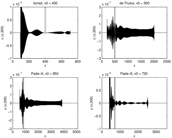
Figure 1: Zoom in of snapshots at $t=300$ of the radiation generated at both sides of a compacton of the $K(2,2)$ equation propagating with $c=1$ numerically calculated using $c_{0}=1$, $\Delta x=0.05$, and $\Delta t=0.1$ by means of Ismail (top left plot), de Frutos (top right plot), Padé-6 (bottom left plot), and Padé-8 (bottom right plot) methods, initially located at, respectively, $x_{0}=400$, 500, 850, and 720.

The more interesting and noticeable property of both backward and forward compacton radiation is their self-similarity. Figures 2, 3, 4, and 5 show the absolute value of both the forward (right plots) and the backward (left ones) radiation for, respectively, Ismail, de Frutos, Padé-6, and Padé-8 methods at time $t=150$ (top plots) and $t=300$ (bottom ones). In the plots of Figs. 2–5, the horizontal axis is selected in order to best illustrate the self-similarity of the wavepacket envelope of both numerically-induced radiations by graphical comparison of the top and bottom plots. As shown in Figs. 2–5 the envelope shape of both the forward and the backward radiations is highly dependent on the method and, not illustrated in the plots, on its parameters $\Delta x$ and $\Delta t$, and the compacton velocity $c$.

A possible origin of the self-similar radiation may be the jump experienced by the second-order derivative of the $K(2,2)$ compacton at their edges. However, extensive numerical simulations using Methods 1–4 show that the self-similarity of the radiation is also present in the propagation of $K(p,p)$ compactons with $k$ continuous derivatives at its both edges, i.e., for $p=(2+k)/k$. The only cases in which the self-similarity is not clearly visible are for $p\gtrapprox 1$, for which the amplitude of the radiation is comparable with the tolerance used in the iterations of the Newton method. In such cases, the radiation near the compacton is degraded by noise, apparently introduced by round-off errors, destroying the self-similarity and, for long-time integrations, blowing up the solution.

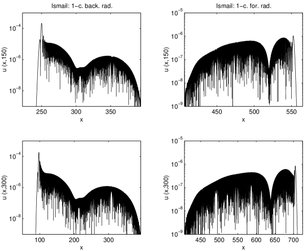
Figure 2: Backward (left plots) and forward (right ones) radiation generated by a compacton of the $K(2,2)$ equation numerically propagating with Ismail method with $\Delta x=0.05$, $\Delta t=0.1$, and $c_{0}=c=1$ at two instants of time, $t=150$ (top plots) and $t=300$ (bottom ones), highlighting their self-similarity.

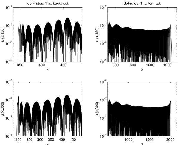
Figure 3: Backward (left plots) and forward (right ones) radiation generated by a compacton of the $K(2,2)$ equation numerically propagating with de Frutos method with $\Delta x=0.05$, $\Delta t=0.1$, and $c_{0}=c=1$ at two instants of time, $t=150$ (top plots) and $t=300$ (bottom ones), highlighting their self-similarity.

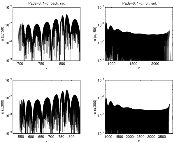
Figure 4: Backward (left plots) and forward (right ones) radiation generated by a compacton of the $K(2,2)$ equation numerically propagating with Padé-6 method with $\Delta x=0.05$, $\Delta t=0.1$, and $c_{0}=c=1$ at two instants of time, $t=150$ (top plots) and $t=300$ (bottom ones), highlighting their self-similarity.

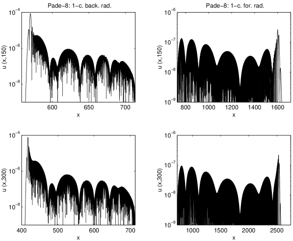
Figure 5: Backward (left plots) and forward (right ones) radiation generated by a compacton of the $K(2,2)$ equation numerically propagating with Padé-8 method with $\Delta x=0.05$, $\Delta t=0.1$, and $c_{0}=c=1$ at two instants of time, $t=150$ (top plots) and $t=300$ (bottom ones), highlighting their self-similarity.

The numerical origin of the spurious radiation observed in the simulations is illustrated in Tables 1 and 2, which show the amplitude of both the backward ($u_{b}$) and forward ($u_{f}$) radiation for the four methods studied in this paper as a function of $\Delta x$ and $\Delta t$, respectively. This amplitude has been determined by finding the first local maximum of the wavepacket starting from the front of the wavepacket using a five point rule, i.e., three nodes where the function increases followed by two nodes where it decreases, being the amplitude value that of the central node. Tables 1 and 2 clearly show that the amplitude of both radiations decreases with decreasing $\Delta x$ but remains practically constant with $\Delta t$. The numerical origin of the radiations appear to be the numerical approximation of the spatial derivatives. The last column of Table 1 shows the exponent $q$ such that the amplitude of the radiations are O​(Δxq), calculated by means of linear regression. This exponent may clarified whether the approximation of either the first or the third derivatives in Eq. (1) is the only responsible of any of these radiations. However, the results shown in Table 1 are not conclusive in this respect and the radiations appear to be the result of the trade-off between the local truncation error of both derivatives. Similar results have been obtained for the other $K(p,p)$ equations studied in this paper.

Table 1: Amplitude at $t=150$ of both the backward ($u_{b}$) and forward ($u_{f}$) radiation for a compacton of the $K(2,2)$ equation with velocity $c=1$ as a function of $\Delta x$ using $\Delta t=0.05$, $c_{0}=c$, and $x\in[0,2500]$. The asterisks indicate solutions which blow up. Linear regression is used to obtain $q$ such that $u_{f}$ and $u_{b}$ are O​(Δxq).

$$\begin{array}[]{|c|c|c|c|c|c|c|c|c|c|}\hline\cr Meth.&\Delta x&0.2&0.1&0.05&0.025&0.0125&q\\ \hline\cr 1&u_{f}&6.54\times 10^{-5}&7.14\times 10^{-6}&1.26\times 10^{-6}&2.24\times 10^{-7}&*&2.7\\ &u_{b}&2.78\times 10^{-3}&6.22\times 10^{-3}&2.94\times 10^{-4}&5.93\times 10^{-5}&*&2.1\\ \hline\cr 2&u_{f}&5.68\times 10^{-6}&7.09\times 10^{-7}&1.61\times 10^{-7}&2.71\times 10^{-8}&8.04\times 10^{-9}&2.4\\ &u_{b}&1.45\times 10^{-5}&2.54\times 10^{-6}&2.60\times 10^{-7}&4.80\times 10^{-8}&1.50\times 10^{-8}&2.6\\ \hline\cr 3&u_{f}&8.32\times 10^{-6}&4.00\times 10^{-7}&8.95\times 10^{-8}&2.11\times 10^{-8}&8.12\times 10^{-9}&2.4\\ &u_{b}&1.84\times 10^{-5}&4.46\times 10^{-6}&3.81\times 10^{-7}&7.43\times 10^{-8}&2.35\times 10^{-8}&2.5\\ \hline\cr 4&u_{f}&1.76\times 10^{-5}&1.64\times 10^{-6}&2.79\times 10^{-7}&4.84\times 10^{-8}&7.23\times 10^{-9}&2.8\\ &u_{b}&4.24\times 10^{-3}&3.17\times 10^{-4}&8.90\times 10^{-5}&2.34\times 10^{-5}&5.97\times 10^{-6}&2.3\\ \hline\cr\end{array}$$

Table 2: Amplitude at $t=150$ of both the backward ($u_{b}$) and forward ($u_{f}$) radiation for a compacton of the $K(2,2)$ equation with velocity $c=1$ as a function of $\Delta t$ using $c_{0}=c$, $\Delta x=0.05$, and $x\in[0,2500]$. Linear regression is used to obtain $q$ such that $u_{f}$ and $u_{b}$ are O​(Δtq).

$$\begin{array}[]{|c|c|c|c|c|c|c|c|c|}\hline\cr Meth.&\Delta t&0.1&0.05&0.025&0.0125&0.00625&q\\ \hline\cr 1&u_{f}&1.04\times 10^{-6}&1.26\times 10^{-6}&1.37\times 10^{-6}&1.40\times 10^{-6}&1.41\times 10^{-6}&-.10\\ &u_{b}&2.17\times 10^{-4}&2.94\times 10^{-4}&1.53\times 10^{-3}&1.44\times 10^{-3}&1.21\times 10^{-3}&-.73\\ \hline\cr 2&u_{f}&1.52\times 10^{-7}&1.61\times 10^{-7}&1.96\times 10^{-7}&2.11\times 10^{-7}&2.16\times 10^{-7}&-.14\\ &u_{b}&2.72\times 10^{-7}&2.60\times 10^{-7}&4.18\times 10^{-7}&7.88\times 10^{-7}&7.70\times 10^{-7}&-.46\\ \hline\cr 3&u_{f}&1.53\times 10^{-7}&8.95\times 10^{-8}&1.11\times 10^{-7}&1.24\times 10^{-7}&1.29\times 10^{-7}&.002\\ &u_{b}&4.11\times 10^{-7}&3.81\times 10^{-7}&1.11\times 10^{-6}&8.71\times 10^{-7}&7.00\times 10^{-7}&-.27\\ \hline\cr 4&u_{f}&2.65\times 10^{-7}&2.79\times 10^{-7}&2.75\times 10^{-7}&2.81\times 10^{-7}&2.93\times 10^{-7}&-.03\\ &u_{b}&8.64\times 10^{-5}&8.90\times 10^{-5}&8.18\times 10^{-5}&8.17\times 10^{-5}&8.08\times 10^{-5}&.030\\ \hline\cr\end{array}$$

The position of the left (right) front of the backward (forward) radiation wavepackets for the Ismail (top left plot), de Frutos (top right plot), Padé-6 (bottom left plot) and Padé-8 (bottom right plot) methods for the $K(2,2)$ equation is shown in Fig. 6. This position has been determined, using linear interpolation, as the “first” point from the outside of the wavepacket, i.e., from left to right (right to left) for backward (forward) radiation, where the amplitude of the solution is equal to an amplitude threshold, the half of the maximum amplitude of the radiation at $t=300$. The four plots in Fig. 6 clearly show a linear evolution of the position of the front for both forward (continuous line) and backward (dashed line) radiations. The velocity of the front, i.e., the slope of these curves, is nearly constant during propagation being negative (positive) for backward (forward) radiation. The constancy of the front velocities has also been observed in the simulations of the $K(p,p)$ equation.

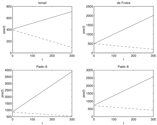
Figure 6: Front velocity evolution of both forward (continuous line) and backward (dashed line) radiations for a $K(2,2)$ compacton numerically propagating as a function of time for Ismail (top left plot), de Frutos (top right), Padé-6 (bottom left) and Padé-8 (bottom right) methods with $\Delta x=0.05$, $\Delta t=0.1$ and $c_{0}=c=1$.

The front velocity of both the forward ($c_{f}$) and the backward ($c_{b}$) wavepackets relative to the velocity of the compacton may be calculated by linear regression from the evolution in time of their positions. Our extensive numerical experiments show that both the forward ($c_{f}$) and backward ($c_{b}$) front velocities are linear functions of the parameter $c_{0}$, being practically independent of the parameters $\Delta x$ and $\Delta t$, and, also nearly independent of $c$ and $p$, for a $K(p,p)$ compacton, with a small percentage increase as $p$ decreases approaching unity.

Table 3 shows both the forward ($c_{f}$) and backward ($c_{b}$) front velocities for $c_{0}=c/2$, $c$, and $2c$, for two values of $\Delta x$ and two values of $\Delta t$. The front velocities depend linearly on $c_{0}$ instead on $c$, in fact, $c_{f}\approx c_{0}$, $5\,c_{0}$, $10\,c_{0}$, and $6\,c_{0}$ for Methods 1–4, respectively, and $c_{b}\approx-c_{0}$ for the four methods. This approximations are better as $\Delta x$ decreases. Let us highlight that both front velocities are relative to that of the compacton, therefore, in a rest frame of reference, where the compacton propagates with its own velocity instead of being stopped by the condition $c_{0}=c$, the backward radiation is generated in the left edge of the compacton at $t=0$ and stretches as it propagates, like a wake left in the track of the compacton during its propagation signaling its initial position in the numerical simulation.

Table 3: Velocity of the front of both the backward and forward radiation for a $K(2,2)$ compacton with velocity $c=1$ as function of $c_{0}$ in numerical simulations with two $\Delta x$, two $\Delta t$, $x\in[0,2500]$ and $t\in[0,100]$.

$$\begin{array}[]{|c|c|c|c|c||c|c|c||c|c|c|}\hline\cr\vrule\lx@intercol\hfil\hfil\lx@intercol\vrule\lx@intercol&\lx@intercol\hfil\Delta x=0.1\hfil\lx@intercol\vrule\lx@intercol\vrule\lx@intercol&\lx@intercol\hfil\Delta x=0.5\hfil\lx@intercol\vrule\lx@intercol\\ \cline{3-11}\cr\vrule\lx@intercol\hfil\hfil\lx@intercol\vrule\lx@intercol&\lx@intercol\hfil\Delta t=0.025\hfil\lx@intercol\vrule\lx@intercol\vrule\lx@intercol&\lx@intercol\hfil\Delta t=0.05\hfil\lx@intercol\vrule\lx@intercol\\ \hline\cr Meth.&c_{0}&1/2&1&2&1/2&1&2&1/2&1&2\\ \hline\cr 1&c_{f}&*&1.02&2.03&*&1.02&2.03&*&1.01&2.02\\ &c_{b}&*&-1.02&-2.03&*&-1.03&-2.04&*&-1.02&-2.03\\ \hline\cr 2&c_{f}&2.55&5.06&10.1&2.56&5.07&10.1&2.53&5.05&*\\ &c_{b}&-0.500&-1.01&-2.01&-0.504&-1.01&-2.02&-0.505&-1.01&*\\ \hline\cr 3&c_{f}&5.09&10.1&20.1&5.09&10.1&20.2&5.06&10.1&*\\ &c_{b}&-0.672&-1.25&-2.05&-0.634&-1.03&-2.02&-0.514&-1.01&*\\ \hline\cr 4&c_{f}&3.12&6.18&12.3&3.12&6.19&12.4&3.10&6.16&*\\ &c_{b}&-0.510&-1.00&-2.01&-0.506&-1.01&-2.02&-0.505&-1.01&*\\ \hline\cr\end{array}$$

Present results suggest that the spatial numerical approximation of the linear term introduced in Eq. (1) in order to stop de compacton may be the responsible of the self-similarity of the envelope of the radiation studied in this paper. Introducing into the modified equation [29] for Method $i$ applied to Eq. (1) the solution $u=u_{c}+u_{r}$, where $u_{c}$ is the compacton (2) and $u_{r}$ is the numerically induced radiation, with $|u_{r}|\ll|u_{c}|$ in the support of the compacton and $u_{c}=0$ outside it, yields

$$\frac{\partial{u_{r}}}{\partial{t}}-c_{0}\,\frac{\mathcal{B}_{i}(e^{\Delta x\,D})}{\mathcal{A}_{i}(e^{\Delta x\,D})}\,u_{r}=\mbox{h.o.t.},$$ (6)

where $D\equiv{\partial{}}/{\partial{x}}$ and h.o.t. stands for higher-order terms. The linear dispersion of this equation is obtained by substitution of $u_{r}=\exp(\mbox{i}\,(k\,x-w_{i}(k)\,t))$ into Eq. (6). The envelope of a wavepacket of radiation propagates with the group velocity, $C_{i}(k)={d{w_{i}(k)}}/{d{k}}$, given by

$$C_{1}(k)=-c_{0}\,\frac{d{}}{d{k}}\frac{\sin(\Delta x\,k)}{\Delta x}=-c_{0}\,\cos(\Delta x\,k),$$

$$C_{2}(k)=-c_{0}\,\frac{d{}}{d{k}}\frac{50\,\sin(\Delta x\,k)+5\,\sin(2\,\Delta x\,k)}{(33+26\,\cos(\Delta x\,k)+\cos(2\,\Delta x\,k))\,\Delta x},$$

$$C_{3}(k)=-c_{0}\,\frac{d{}}{d{k}}\frac{100\,\sin(\Delta x\,k)+10\,\sin(2\,\Delta x\,k)}{(63+56\,\cos(\Delta x\,k)+\cos(2\,\Delta x\,k))\,\Delta x},$$

$$C_{4}(k)=-c_{0}\,\frac{d{}}{d{k}}\frac{160\,\sin(\Delta x\,k)+25\,\sin(2\,\Delta x\,k)}{(108+96\,\cos(\Delta x\,k)+6\,\cos(2\,\Delta x\,k))\,\Delta x},$$

for Methods 1–4, respectively, which are plotted in Figure 7 as a function of the normalized wavenumber $\alpha$, given by $k=\alpha\,k_{\max}$ where the highest wavenumber in the spatial grid is $k_{\max}=\pi/\Delta x$. The discrete Fourier transform of the forward radiation shows that its spectrum is concentrated around the highest wavenumber, therefore, its front velocity is given by $C_{i}(k_{\max})=c_{0}$, $5\,c_{0}$, $10\,c_{0}$, and $6.11\,c_{0}$, for Methods 1–4, respectively. The spectrum for the backward radiation presents several peaks of low frequency accompanied with a smaller peak at the highest wavenumber, therefore, its front velocity is given approximately by $C_{i}(k_{\max}/10)\approx-c_{0}$, for Methods 1–4. These results are in good agreement with Table 3 and further results for the $K(p,p)$ equation omitted here for brevity.

Figure 7: Group velocity of Method 1 (solid line), 2 (dashed line), 3 (dash-dotted line), and 4 (dotted line) for the linear Eq. (6) as a function of the normalized wavenumber $\alpha$, such that $k=\alpha\,\pi/\Delta x$.

Equation (6) is not the only responsible of the numerically induced self-similar radiations by the $K(p,p)$ compactons since it is easy to show that it has no self-similar solutions. Moreover, the numerical solution by all the methods studied in this paper blow ups when $c_{0}$ either has a negative value ($c_{0}\,c<0$) or has a value very different from $c$ (either $|c_{0}|\ll|c|$, or $|c_{0}|\gg|c|$). This result, found in a large number of simulations and illustrated in the last column of Table 3, was unnoticed by the authors of Ref. [20], whose first introduced the linear term in Eq. (1), and in further references [24, 26, 27]. Furthermore, a linear stability analysis of the semidiscrete Eq. (6) shows its unconditional stability, independently of the value of $c_{0}$, so the roots of this instability must be in the nonlinear terms not considered in it.

The self-similarity of both the forward and the backward radiation requires that their analytical expressions be self-similar functions which may be analytically written as, respectively,

$$u(x,t)=t^{-\varrho_{f}}\,u_{f}\left(\frac{x-x_{f}-c\,t}{c_{f}\,t}\right),\qquad x_{f}+c\,t\leq x<\infty,$$ (7)

$$u(x,t)=t^{-\varrho_{b}}\,u_{b}\left(\frac{x-x_{b}}{|c_{b}|\,t}\right),\qquad\qquad-\infty<x\leq x_{b}+c\,t,$$ (8)

where $x_{b}=x_{0}-{\pi}/({2\,\beta})$ and $x_{f}=x_{0}+{\pi}/({2\,\beta})$ are, respectively, the left and right extremes of the compacton solution, $\varrho_{b}$ and $\varrho_{f}$ are the scaling exponents for, respectively, the forward and the backward radiation, and $u_{f}$ and $u_{b}$ are the shapes of, respectively, the forward and backward wavepackets. In order to verify that the scaling exponents in Eqs. (7) and (8) are really constant, the temporal evolution of the amplitude of both radiations must be studied. Figure 8 shows that this amplitude changes a little in the first steps of time but yields a very smooth decreasing curve as time progresses, being approximately linear in the logarithmic scale of the plots. Therefore, the temporal evolution of the amplitude is asymptotically exponential in time. Similar results have been also obtained for other $K(p,p)$ compactons and/or mesh parameters.

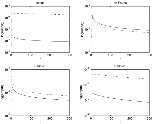
Figure 8: Amplitude evolution of both forward (continuous line) and backward (dashed line) radiations as a function of time for Ismail (top left plot), de Frutos (top right), Padé-6 (bottom left) and Padé-8 (bottom right) methods applied to the $K(2,2)$ equation.

Tables 4 and 5 show the scaling exponents in Eqs. (7) and (8) as function of $\Delta x$ and $c_{0}=c$, respectively, since our extensive set of simulations show that the time step has no significant influence on the results. The scaling exponents in these tables have been determined by using linear regression of the temporal evolution of the “mean” amplitude of the envelope of the wavepackets, i.e., the mean of the absolute value of the amplitude of the solution in the intervals $[x_{b},x_{b}+c\,t]$ and $[x_{f}+c\,t,x_{f}+(c+c_{f})\,t]$ for the backward and forward radiations, respectively. To avoid the effects of the initial transient, where the self-similarity of the wavepackets is not properly defined due to the aliasing errors introduced by the sampling of the solution, the first 25% of the solution is not considered in the linear regression.

Table 4: Scaling exponent of both forward and backward radiations for the Ismail, de Frutos, Padé-6, and Padé-8 methods for a $K(2,2)$ compacton in numerical simulations with $\Delta t=0.05$ and $c_{0}=c=1$ as a function of $\Delta x$, calculated using a linear regression of the evolution in time of the mean amplitude in the interval $t\in[75,300]$.

$$\begin{array}[]{|c|c|c|c|c|c|c|c|c|}\hline\cr&\Delta x&0.2&0.1&0.05&0.025&0.0125\\ \hline\cr\mbox{Ismail}&\varrho_{f}&0.487&0.453&0.503&0.482&0.464\\ &\varrho_{b}&0.487&0.924&0.977&1.05&1.18\\ \hline\cr\mbox{de Frutos}&\varrho_{f}&0.501&0.497&0.498&0.499&0.500\\ &\varrho_{b}&0.549&0.547&0.514&0.513&0.505\\ \hline\cr\mbox{Pad\'{e}-6}&\varrho_{f}&0.492&0.494&0.496&0.498&0.608\\ &\varrho_{b}&0.532&0.537&0.500&0.506&0.612\\ \hline\cr\mbox{Pad\'{e}-8}&\varrho_{f}&0.481&0.513&0.527&0.556&0.520\\ &\varrho_{b}&0.077&0.774&0.931&0.891&0.875\\ \hline\cr\end{array}$$

Tables 4 and 5 show that the scaling factor $\varrho_{f}$ is approximately equal to 0.5 for all the four methods studied in this paper, nearly independent of both $\Delta x$ and $c_{0}=c$, respectively, with the largest dispersion associated to Padé-8 and Ismail methods. Tables 4 and 5 also show that the scaling factor $\varrho_{b}$ is approximately equal to 0.5 for the de Frutos and Padé-6 methods, to 0.9 for the Padé-8 method, and to 1.0 for the Ismail method, with a small decrement as $c$ grows, for both the Padé-8 and Ismail methods. For the last two methods the dispersion is large, although diminish if the first column of Tables 4 and 5 is not taken into account since it corresponds to a large $\Delta x$ and presents very noticeable aliasing errors.

Table 5: Scaling exponent of both forward and backward radiations for the Ismail, de Frutos, Padé-6, and Padé-8 methods for a $K(2,2)$ compacton in numerical simulations with $\Delta t=0.05$ and $\Delta x=0.05$ as a function of $c_{0}=c$, calculated using a linear regression of the evolution in time of the mean amplitude in the interval $t\in[75,300]$.

$$\begin{array}[]{|c|c|c|c|c|c|c|c|c|c|}\hline\cr&c_{0}&0.1&0.2&0.5&1&1.5&2&5\\ \hline\cr\mbox{Ismail}&\varrho_{f}&0.157&0.512&0.519&0.503&0.492&0.487&0.477\\ &\varrho_{b}&2.408&1.18&1.07&0.977&0.827&0.794&0.778\\ \hline\cr\mbox{de Frutos}&\varrho_{f}&0.492&0.494&0.496&0.510&0.495&0.495&0.498\\ &\varrho_{b}&0.542&0.552&0.505&0.511&0.499&0.495&0.479\\ \hline\cr\mbox{Pad\'{e}-6}&\varrho_{f}&0.487&0.489&0.491&0.496&0.489&0.490&0.489\\ &\varrho_{b}&0.561&0.507&0.437&0.500&0.496&0.507&0.504\\ \hline\cr\mbox{Pad\'{e}-8}&\varrho_{f}&0.534&0.496&0.562&0.527&0.530&0.507&0.482\\ &\varrho_{b}&0.433&0.962&0.995&0.931&0.899&0.760&0.483\\ \hline\cr\end{array}$$

4 Conclusions

The propagation of compactons of the Rosenau-Hyman $K(p,p)$ equation has been studied by means of four numerical methods showing the appearance of numerically-induced radiation. Both backward and forward wavepackets are generated from the compacton with a clear self-similar shape, illustrated by means of properly scaling of the figures. The parameters characterizing these wavepackets have been numerically determined. An analytical model, based on the linearization of $K(p,p)$ equation has been used in order to approximate the front velocities of the forward wavepackets relative to that of the compacton. The front velocity of the backward wavepacket is approximately equal to that of the compacton but with opposite sign. Both forward and backward front velocities are practically independent of the parameters $\Delta x$ and $\Delta t$ of the numerical method. The evolution in time of the mean amplitude of the wavepackets shows its exponential decreasing in time, suggesting an ansatz for both the backward and forward wavepackets corresponding to self-similar functions characterized by scaling exponents, which have been numerically calculated for both radiations by means of the linear regression of the logarithm of the mean amplitude, showing that its value is approximately constant as a function of both the mesh grid size and the compacton velocity.

The scaling exponents approximately equal to $1/2$ for the amplitude evolution of the envelope of both the forward and the backward radiations suggest that they may be analytically approximated for weak nonlinearity (valid for the radiation but not for the compactons) by a nonlinear (cubic) Schrödinger equation. This analysis is in progress. Asymptotic analysis using the method of modified equations applied to the four numerical methods studied in this paper may also be useful in the characterization of the radiation wavepackets found here. In fact, the analytical explanation of both the generation of the self-similar radiations and the blow-up of the solution for some $c_{0}$ are very interesting open problems.

References

• [1] P. Rosenau and J. M. Hyman, Compactons: Solitons with finite wavelength, Phys. Rev. Lett., 70(5) (1993) 564–567.
• [2] P. Rosenau, On a class of nonlinear dispersive-dissipative interactions, Physica D, 123(1–4) (1998) 525–546.
• [3] A. Ludu and J. P. Draayer, Patterns on liquid surfaces: cnoidal waves, compactons and scaling, Physica D, 123() (1998) 82–91.
• [4] A. L. Bertozzi and M. Pugh, The lubrication approximation for thin viscous films: regularity and long time behavior of weak solutions, Commun. Pure Appl. Math., 49(2) (1996) 85–123.
• [5] A. S. Kovalev and M. V. Gvozdikova, Bose gas with nontrivial particle interaction and semiclassical interpretation of exotic solitons, Low Temp. Phys., 24(7) (1998) 484–488.
• [6] R. H. J. Grimshaw, L. A. Ostrovsky, V. I. Shrira, and Y. A. Stepanyants, Long nonlinear surface and internal gravity waves in a rotating ocean, Surv. Geophys., 19(4) (1998) 289–338.
• [7] V. Kardashov, S. Einav, Y. Okrent, and T. Kardashov, Nonlinear reaction-diffusion models of self-organization and deterministic chaos: Theory and possible applications to description of electrical cardiac activity and cardiovascular circulation, Discrete Dyn. Nat. Soc., 2006 (2006) Art. 98959.
• [8] G. Simpson, M. Spiegelman, and M. I. Weinstein, Degenerate dispersive equations arising in the study of magma dynamics, Nonlinearity, 20 (2007) 21–49.
• [9] E. C. Caparelli, V. V. Dodonov, and S. S. Mizrahi, Finite-length soliton solutions of the local homogeneous nonlinear Schr dinger equation, Phys. Scr., 58 (1998) 417–420.
• [10] S. Dusuel, P. Michaux, and M. Remoissenet, From kinks to compactonlike kinks, Phys. Rev. E, 57(2) (1998) 2320–2326.
• [11] J. C. Comte, Compact traveling kinks and pulses, Chaos Solitons Fractals, 14 (2002) 1193–1199.
• [12] J. C. Comte and P. Marquié, Compact-like kink in real electrical reaction-diffusion chain, Chaos Solitons Fractals, 29 (2006) 307–312.
• [13] J. E. Prilepsky, A. S. Kovalev, M. Johansson, and Y. S. Kivshar, Magnetic polarons in one-dimensional antiferromagnetic chains, Phys. Rev. B, 74 (2006) Art. 132404.
• [14] P. Rosenau and A. Pikovsky, Phase compactons in chains of dispersively coupled oscillators, Phys. Rev. Lett., 94 (2005) Art. 174102.
• [15] A. Pikovsky and P. Rosenau, Phase compactons, Physica D, 218 (2006) 56–69.
• [16] P. Rosenau, Compact and noncompact dispersive patterns, Phys. Lett. A, 275(3) (2000) 193–203.
• [17] F. Cooper, A. Khare, and A. Saxena, Exact elliptic compactons in generalized Korteweg De Vries equations, Complexity, 11(6) (2006) 30–34.
• [18] P. Rosenau, On a model equation of traveling and stationary compactons, Phys. Lett. A, 356(1) (2006) 44–50.
• [19] P. Rosenau, J. M. Hyman, and M. Staley, Multidimensional compactons, Phys. Rev. Lett., 98 (2007) Art. 024101.
• [20] J. de Frutos, M. A. López-Marcos, and J. M. Sanz-Serna, A finite difference scheme for the $K(2,2)$ compacton equation, J. Comput. Phys., 120(2) (1995) 248–252.
• [21] P. Saucez, A. V. Wouwer, W. E. Schiesser, and P. Zegeling, Method of lines study of nonlinear dispersive waves, J. Comput. Appl. Math., 168(1-2) (2004) 413–423.
• [22] A. Chertock and D. Levy, Particle methods for dispersive equations, J. Comput. Phys., 171(2) (2001) 708–730.
• [23] F. Cooper, J. M. Hyman, and A. Khare, Compacton solutions in a class of generalized fifth-order Korteweg-de Vries equations, Phys. Rev. E, 64 (2001) Art. 026608.
• [24] F. Rus and F. R. Villatoro, Padé Numerical method for the Rosenau-Hyman compacton equation, Math. Comput. Simul. (2007), doi:10.1016/ j.matcom.2007.01.016.
• [25] D. Levy, C. W. Shu, and J. Yan, Local discontinuous Galerkin methods for nonlinear dispersive equations, J. Comput. Phys., 196(2) (2004) 751–772.
• [26] M. S. Ismail and T. R. Taha, A numerical study of compactons, Math. Comput. Simul., 47(6) (1998) 519–530.
• [27] H. Han and Z. Xu, Numerical solitons of generalized Korteweg-de Vries equations, Appl. Math. Comput., 186(1) (2007) 483–489.
• [28] J. Garralón, F. Rus, and F. R. Villatoro, Compacton numerically-induced radiation in a fourth-order finite element method, WSEAS T. Math., 5(1) (2006) 89–96.
• [29] F. R. Villatoro and J. I. Ramos, On the method of modified equations. I: Asymptotic analysis of the Euler forward difference method, Appl. Math. Comput., 103(2-3) (1999) 111–139.