A modified Next Reaction Method for simulating chemical systems with time dependent propensities and delays

Abstract

Chemical reaction systems with a low to moderate number of molecules are typically modeled as discrete jump Markov processes. These systems are oftentimes simulated with methods that produce statistically exact sample paths such as the Gillespie Algorithm or the Next Reaction Method. In this paper we make explicit use of the fact that the initiation times of the reactions can be represented as the firing times of independent, unit rate Poisson processes with internal times given by integrated propensity functions. Using this representation we derive a modified Next Reaction Method and, in a way that achieves efficiency over existing approaches for exact simulation, extend it to systems with time dependent propensities as well as to systems with delays.

I Introduction

Due to advances in the knowledge of cellular systems, where there are low to moderate numbers of molecules of certain species, there has been a renewed interest in modeling chemical systems as discrete and stochastic as opposed to deterministic and continuous. ^{1, 2, 3, 4} Because of the intrinsic stochasticity at this level, understanding of a given system is gained through knowledge of the distribution of the state of the system at a given time. As it is typically impracticable to analytically solve for the distribution of the state of the system at a particular time for all but the simplest of examples, simulation methods have been developed that generate statistically exact sample paths so as to approximate the distribution. The two most widely used exact simulation methods are the original Gillespie Algorithm ^{5, 6} and the Next Reaction Method of Gibson and Bruck. ⁷

In this paper, we will explicitly represent the reaction times of discrete stochastic chemical systems as the firing times of independent, unit rate Poisson processes with internal times given by integrated propensity functions. Such a representation is not novel and is called a random time change representation in the mathematics literature. See, for example, Refs. ⁸, ⁹, ¹⁰. However, using such a representation in an explicit attempt to develop new simulation methods has a number of benefits that have seemingly not been explored in the chemistry literature. First, the representation will naturally lead us to a modified version of the Next Reaction Method. ⁷ Second, the modified Next Reaction Method will be shown to be the natural choice for simulating systems with propensities that depend explicitly on time (such as systems with variable temperature or cell volume). Third, we will be able to easily extend our modified Next Reaction Method to systems that allow delays between the initiation and completion of reactions in a manner that achieves efficiency over existing methods. More precisely, in our modified Next Reaction Method for systems with delays no random numbers or computations will be wasted (such as happens in the method of Bratsun et al. ¹¹ and Barrio et al. ¹²) (see Section VI), and there will be no need for the complicated machinery of the method developed by Cai ¹³ (see Section VI) in the handling of the stored delayed reactions. We note that the ideas we use to develop our modified Next Reaction Method are analogous to the theories of generalized semi-Markov processes ^{14, 15, 16} and stochastic Petri nets ¹⁷, and can also be extended to develop new accurate and efficient approximate tau-leaping methods. ¹⁸

The outline of the paper is as follows. In Section II we briefly present the original Gillespie Algorithm. In Section III we introduce our representation of the reaction times as the firing times of independent, unit rate Poisson processes with internal time given by integrated propensity functions. In Section IV we rederive the Next Reaction Method and derive a modified Next Reaction Method using the representation detailed in Section III. In Section V we consider systems with propensities that depend explicitly on time and conclude that our modified Next Reaction Method is the preferable algorithm to use in such cases. In Section VI we consider systems in which there is a delay between the initiation and completion of some of the reactions and develop a new algorithm for simulating such systems that is an extension of our modified Next Reaction Method.

II The Gillespie Algorithm

Consider a system consisting of $N\geq 1$ chemical species, $\{X_{1},\dots,X_{N}\}$, undergoing $M\geq 1$ chemical reactions, each of which is equipped with a propensity function (or intensity function in the mathematics literature), $a_{k}(X)$. For the time being, assume that the time between the initiation and the completion of each reaction is negligible. To accurately simulate the time evolution of the number of each species, $X(t)=\{X_{1}(t),\dots,X_{N}(t)\}\in\mathbb{N}_{\geq 0}^{N}$, one needs to be able to calculate 1) how much time will pass before the next reaction takes place (i.e. initiates and completes) and 2) which reaction takes place at that future time. One can then simulate statistically exact sample paths for the system of interest. The following assumption, sometimes called the fundamental premise of chemical kinetics, is based upon physical principles and serves as the base assumption for simulation methods of chemically reacting systems: ⁶

$$\begin{split}a_{k}(X(t))\Delta t+o(\Delta t)=\ &\hbox{the probability that reaction $k$}\\ &\hbox{takes place in a small time interval $[t,t+\Delta t)$},\end{split}$$ (1)

where $o(\Delta t)/\Delta t\to 0$ as $\Delta t\to 0$. Based upon the assumption (1), the time until the next reaction, $\Delta$, is exponentially distributed with parameter $a_{0}(X(t))=\sum_{k=0}^{M}a_{k}(X(t))$ and the probability that the next reaction is the $k$th is $a_{k}(X(t))/a_{0}(X(t))$. These observations form the foundation for the well known Gillespie Algorithm. ^{5, 6}

Algorithm 1.

(Gillespie Algorithm)

1. Initialize. Set the initial number of molecules of each species and set $t=0$.

2. Calculate the propensity function, $a_{k}$, for each reaction.

3. Set $a_{0}=\sum_{k=1}^{M}a_{k}$.

4. Generate two independent uniform(0,1) random numbers $r_{1}$ and $r_{2}$.

5. Set $\Delta=1/a_{0}\ln(1/r1)$ (equivalent to drawing an exponential random variable with parameter $a_{0}$).

6. Find $\mu\in[1,\dots,M]$ such that

   $$\sum_{k=1}^{\mu-1}a_{k}<r_{2}a_{0}\leq\sum_{k=1}^{\mu}a_{k},$$

   which is equivalent to choosing from reactions $[1,\dots,M]$ with the $k$th reaction having probability $a_{k}/a_{0}$.

7. Set $t=t+\Delta$ and update the number of each molecular species according to reaction $\mu$.

8. Return to step 2 or quit.

We point out that the Gillespie Algorithm uses two random numbers per step. The first is used to find when the next reaction occurs and the second is used to determine which reaction occurs at that time. In Section IV we will demonstrate how the Next Reaction Method generates exact sample paths while only needing one random number per step.

III Representation using Poisson processes

We will explicitly represent the reaction times of chemical systems as the firing times of Poisson processes with internal times given by integrated propensity functions. ^{8, 9, 10} Using such a representation allows us to consider the system as a whole via a stochastic integral equation as opposed to solely considering how to calculate when the next reaction occurs and which reaction occurs at that time. The benefits of such a representation will stem from the fact that the randomness in the model is separated from the state of the system.

Let $\nu_{k},\nu_{k}^{\prime}\in\mathbb{N}_{\geq 0}^{n}$ be the vectors representing the number of each species consumed and created in the $k$th reaction, respectively. Then, if $R_{k}(t)$ is the number of times that the $k$th reaction has taken place up to time $t$, the state of the system at time $t$ is

$$X(t)=X(0)+\sum_{k=1}^{M}R_{k}(t)(\nu_{k}^{\prime}-\nu_{k}).$$ (2)

However, based upon the assumption (1), $R_{k}(t)$ is a counting process with intensity $a_{k}(X(t))$ such that Prob$(R_{k}(t+\Delta t)-R_{k}(t)=1)=a_{k}(X(t))\Delta t$ for small $\Delta t$. Therefore,

$$R_{k}(t)=Y_{k}\left(\int_{0}^{t}a_{k}(X(s))ds\right),$$ (3)

where the $Y_{k}$ are independent, unit rate Poisson processes. Thus, $X(t)$ can be represented as the solution to the following equation:

$$X(t)=X(0)+\sum_{k=1}^{M}Y_{k}\left(\int_{0}^{t}a_{k}(X(s))ds\right)(\nu_{k}^{\prime}-\nu_{k}).$$ (4)

Note that the state of the system, $X(s)$, and hence each propensity function $a_{k}(X(s))$, is constant between reaction times. In Section V we will consider systems in which the propensity functions are not constant between reactions, such as arise due to changes in temperature or cellular volume.

We make two points that are crucial to an understanding of how different simulation methods arise from equation (4). First, all of the randomness in the system is encapsulated in the $Y_{k}$’s and has therefore been separated from the state of the system. Thus, since the system (4) only changes when one of the $Y_{k}$’s change, the relevant question of each simulation algorithm is how to efficiently calculate the firing times of each $Y_{k}$ and how to translate that information into reaction times for the chemical system. Second, there are actually $M+1$ relevant time frames in the system. The first time frame is the actual, or absolute time, $t$. However, each Poisson process $Y_{k}$ brings its own time frame. More specifically, if we define $T_{k}(t)=\int_{0}^{t}a_{k}(X(s))ds$ for each $k$, then it is relevant for us to consider $Y_{k}(T_{k}(t))$. We will call $T_{k}(t)$ the “internal time” for reaction $k$.

Definition 1.

For each $k\leq M$, $T_{k}(t)=\int_{0}^{t}a_{k}(X(s))ds$ is the internal time of the Poisson process $Y_{k}$ of equation (4).

We will use the internal times of the system in an analogous manor to the use of “clocks” in the theory of generalized semi-Markov processes. ^{14, 15, 16}

We now formulate the Gillespie Algorithm (Algorithm 1) in terms of equation (4). At time $t$, we know the state of the system, $X(t)$, the propensity functions, $a_{k}(X(t))$, and the internal times, $T_{k}(t)$. Calculating 1) how much time will pass before the next reaction takes place and 2) which reaction takes place at that future time is equivalent to calculating 1) how much time passes before one of the Poisson processes, $Y_{k}$, fires and 2) which $Y_{k}$ fires at that later time. Combining the previous statement with the fact that the intensities of the Poisson processes are $a_{k}(X(t))$ yields one step of the Gillespie algorithm. Use of the loss of memory property for Poisson processes (which negates knowledge of the internal times $T_{k}(t)$) allows us to perform subsequent steps independently of previous steps.

Note that in the Gillespie Algorithm the firing times of the individual processes $Y_{k}$ were calculated by first finding the time required until any of them fired, and then calculating which reaction fired at that future time. In the next section we show how the Next Reaction Method and our modified Next Reaction Method first calculates when each of the $Y_{k}$ fires next, and then finds the specific reaction that fires by taking the minimum of such times. By not invoking the loss of memory property (and, hence, differentiating themselves from the First Reaction Method ⁶), the Next Reaction Method and modified Next Reaction Method make use of the internal times $T_{k}(t)$ to nearly cut in half the number of random variables needed per simulation.

IV A modified Next Reaction Method

We again consider the system (4). At time $t$ we know the state of the system $X=X(t)$, the propensity functions $a_{k}=a_{k}(X(t))$, and the internal times $T_{k}=T_{k}(t)$. We also assume that we know $\Delta t_{k}$, the amount of absolute time that must pass in order for the $k$th reaction to fire assuming that $a_{k}$ stays constant over the interval $[t,t+\Delta t_{k})$. Therefore, $\tau_{k}=t+\Delta t_{k}$ is the time of the next firing of the $k$th reaction if no other reactions fire first. Note that if $t=0$ and this is the first step in the simulation of the system (and so $T_{k}=0$), finding each $\Delta t_{k}$ is equivalent to taking a draw from an exponential random variable with parameter $a_{k}$. Because we know $\Delta t_{k}$, the internal time at which reaction $k$ fires is given by $T_{k}+a_{k}\Delta t_{k}$. In order to simulate one step, we now note that the next reaction occurs after a time period of $\Delta=\min_{k}\{\Delta t_{k}\}$, and the reaction that fires is the one for which the minimum is achieved, $\mu$ say. Therefore, we may update the system according to reaction $\mu$, update the absolute time by adding $\Delta$ and update the internal times by adding $a_{k}\Delta$ to $T_{k}$, for each $k$.

For the moment we denote $\overline{t}=t+\Delta$ and the updated propensity functions by $\overline{a}_{k}$. The relevant question now is: for each $k$, what is the new absolute time of the firing of $Y_{k}$, $\overline{\tau}_{k}$, assuming no other reaction fires first? For reaction $\mu$, we must generate its next firing time from an exponential random variable with parameter $\overline{a}_{k}$. For $k\neq\mu$ we note that, in general, the new absolute firing times will not be the same as the old because the propensity functions have changed. However, the internal time of the next firing of $Y_{k}$ has not changed and is still given by $T_{k}(t)+a_{k}\Delta t_{k}$. We also know that the updated internal time of $Y_{k}$ is given by $T_{k}(\overline{t})=T_{k}(t)+\Delta a_{k}$. Therefore, the amount of internal time that must pass before the $k$th reaction fires is given as the difference

$$(T_{k}(t)+a_{k}\Delta t_{k})-(T_{k}(t)+\Delta a_{k})=a_{k}(\Delta t_{k}-\Delta).$$

Thus, the amount of absolute time that must pass before the $k$th reaction channel fires, $\Delta\overline{t}_{k}$, is given as the solution to $\overline{a}_{k}\Delta\overline{t}_{k}=a_{k}(\Delta t_{k}-\Delta)$, and so

$$\Delta\overline{t}_{k}=\frac{a_{k}}{\overline{a}_{k}}(\Delta t_{k}-\Delta).$$

Thus, we see that

$$\overline{\tau}_{k}=\frac{a_{k}}{\overline{a}_{k}}(\Delta t_{k}-\Delta)+\overline{t}=\frac{a_{k}}{\overline{a}_{k}}((t+\Delta t_{k})-(t+\Delta))+\overline{t}=\frac{a_{k}}{\overline{a}_{k}}(\tau_{k}-\overline{t})+\overline{t}.$$

We have therefore found the absolute times of the next firings of reactions $k\neq\mu$ without having to generate any new random numbers. Repeated application of the above ideas yields the Next Reaction Method. ⁷

Algorithm 2.

(The Next Reaction Method)

1. Initialize. Set the initial number of molecules of each species and set $t=0$.

2. Calculate the propensity function, $a_{k}$, for each reaction.

3. Generate $M$ independent, uniform(0,1) random numbers $r_{k}$.

4. Set $\tau_{k}=1/a_{k}\ln(1/r_{k})$.

5. Set $t=\min_{k}\{\tau_{k}\}$ and let $\tau_{\mu}$ be the time where the minimum is realized.

6. Update the number of each molecular species according to reaction $\mu$.

7. Recalculate the propensity functions for each reaction and denote by $\overline{a}_{k}$.

8. For each $k\neq\mu$, set $\tau_{k}=(a_{k}/\overline{a}_{k})(\tau_{k}-t)+t.$

9. For reaction $\mu$, let $r$ be uniform(0,1) and set $\tau_{\mu}=1/\overline{a}_{\mu}\ln(1/r)+t$.

10. For each $k$, set $a_{k}=\overline{a}_{k}$.

11. Return to step 5 or quit.

Note that after the first timestep is taken in the Next Reaction Method, all subsequent timesteps only demand one random number to be generated. This is compared with two random numbers needed for each step of the original Gillespie Algorithm (Algorithm 1). We also note that the Next Reaction Method was originally developed with the notion of a dependency graph and a priority queue in order to increase computational efficiency (see Ref. ⁷ for full details). The dependency graph is used in order to only update the propensities that actually change during an iteration (and thereby cut down on unnecessary calculations) and the priority queue was used to quickly determine the minimum value in Step 5. We have omitted the details of these items as they are not necessary for an understanding of the algorithm itself. However, we point out that the use of a dependency graph in order to efficiently update the propensity functions is useful in any of the algorithms presented in this paper, and not just to the Next Reaction Method.

We now present an algorithm that is completely equivalent to Algorithm 2, but makes more explicit use of the internal times $T_{k}$. In the following algorithm, we will denote by $P_{k}$ the first firing time of $Y_{k}$, in the time frame of $Y_{k}$, that is strictly larger than $T_{k}$. That is, $P_{k}=\min\{s>T_{k}:Y_{k}(s)>Y(T_{k})\}$. The main idea of the following algorithm is that by equation (4) the value

$$\Delta t_{k}=(1/a_{k})(P_{k}-T_{k})$$ (5)

gives the amount of absolute time needed until the Poisson process $Y_{k}$ fires assuming that $a_{k}$ remains constant. Of course, $a_{k}$ does remain constant until the next reaction takes place. Therefore, a minimum of the different $\Delta t_{k}$ gives the time until the next reaction takes place. Thus, if we keep track of $P_{k}$ and $T_{k}$ explicitly, we can simulate the systems without the time conversions of step 8 of Algorithm 2.

Algorithm 3.

(Modified Next Reaction Method)

1. Initialize. Set the initial number of molecules of each species. Set $t=0$. For each $k$, set $P_{k}=0$ and $T_{k}=0$.

2. Calculate the propensity function, $a_{k}$ for each reaction.

3. Generate $M$ independent, uniform(0,1) random numbers $r_{k}$.

4. Set $P_{k}=\ln(1/r_{k})$.

5. Set $\Delta t_{k}=(P_{k}-T_{k})/a_{k}$.

6. Set $\Delta=\min_{k}\{\Delta t_{k}\}$ and let $\Delta t_{\mu}$ be the time where the minimum is realized.

7. Set $t=t+\Delta$ and update the number of each molecular species according to reaction $\mu$.

8. For each $k$, set $T_{k}=T_{k}+a_{k}\Delta$.

9. For reaction $\mu$, let $r$ be uniform(0,1) and set $P_{\mu}=P_{\mu}+\ln(1/r)$.

10. Recalculate the propensity functions, $a_{k}$.

11. Return to step 5 or quit.

We note that Algorithms 2 and 3 have the same simulation speeds on all systems that we have tested. This was expected as the two are equivalent. However, as will be shown in the next section, Algorithm 3 extends itself to systems with time dependent rate constants in a smooth way, whereas Algorithm 2 does not. We also point out another nice quality of Algorithms 2 and 3. Suppose that a system is governed by equation (4) except that the $Y_{k}$’s are no longer Poisson processes. That is, we suppose that the reactions do not have exponential waiting times, but have waiting times given by some other distribution. To modify Algorithms 2 and 3 to handle such a situation, one solely needs to change steps 4 and 9 in each so that the waiting times are drawn from the correct distribution.

V Time dependent propensity functions

Due to changes in temperature and/or volume, the rate constants of a (bio)chemical system may change in time. Therefore, the propensity functions will no longer be constant between reactions. That is, $a_{k}(t)=a_{k}(X(t),t),$ and the full system is given by

$$X(t)=X(0)+\sum_{k=1}^{M}Y_{k}\left(\int_{0}^{t}a_{k}(X(s),s)ds\right)(\nu_{k}^{\prime}-\nu_{k}),$$ (6)

where the $Y_{k}$ are independent, unit rate Poisson processes. We consider how to simulate system (6) using the Gillespie Algorithm, the Next Reaction Method, and our modified Next Reaction Method.

The Gillespie Algorithm. At time $t$ we know the state of the system, $X(t)$, and, until the next reaction takes place, the propensity functions $a_{k}(X(t),s)$, for $s>t$. When the propensity functions depended only on the state of the system the Gillespie Algorithm calculated the time until the next reaction by considering the first firing time of $M$ time-homogeneous Poisson processes. However, we now need to calculate the first firing time of $M$ time-inhomogeneous Poisson processes. It is a simple exercise to show that the amount of time that must pass until the next reaction takes place, $\Delta$, has distribution function

$$1-\exp\left(-\sum_{k=1}^{M}\int_{t}^{t+\Delta}a_{k}(X(t),s)ds\right).$$ (7)

Note that $X(t)$ is constant in the above integrals because no reactions take place within the time interval $[t,t+\Delta)$. Using equation (7), $\Delta$ is found by first letting $r$ be uniform$(0,1)$ and then solving the following equation:

$$\sum_{k=1}^{M}\int_{t}^{t+\Delta}a_{k}(X(t),s)ds=\ln(1/r).$$ (8)

In Appendix A we show that the reaction that fires at that time will be chosen according to the probabilities $a_{k}(X(t),t+\Delta)/a_{0}$, where $a_{0}=\sum_{k=1}^{M}a_{k}(X(t),t+\Delta)$. Solving equation (8) either analytically or numerically will be extremely difficult and time consuming in all but the simplest of cases.

The Next Reaction Method. We begin by considering the first step of the Next Reaction Method. At time $t=0$, we need to know the first firing times of independent, inhomogeneous Poisson processes. Therefore, we calculate the time that the $k$th reaction channel will fire (assuming no other reaction fires first) by solving for $\tau_{k}$ from:

$$\int_{0}^{\tau_{k}}a_{k}(X(0),s)ds=\ln(1/r_{k}),$$ (9)

where $r_{k}$ is uniform$(0,1)$. Equation (9) can be solved either analytically or numerically. Say that reaction $\mu$ is the first to fire and does so at time $t$. It is clear that to calculate the next firing time of reaction $\mu$ we will need to generate another uniform$(0,1)$ random variable $r_{\mu}$ and solve

$$\int_{t}^{\tau_{\mu}}a_{k}(X(t),s)ds=\ln(1/r_{\mu}).$$

What is less clear is how to reuse the information contained in $\tau_{k}$ for $k\neq\mu$.

Proceeding as in Ref. ⁷, denote by $F_{n,a}$ the distribution function for the $n$th firing of a reaction, where $a$ is some parameter of the function. Gibson and Bruck prove the following:

Theorem V.1 (Gibson and Bruck’s generation of next firing time ⁷).

Let $\tau$ be a random number generated according to an arbitrary distribution with parameter $a_{n}$ and distribution function $F_{a_{n},n}$. Suppose the current simulation time is $t_{n}$, and the new parameter (after a step in the system in which this reaction did not fire) is $a_{n+1}$. Then the transformation

$$\tau^{*}=F^{-1}_{a_{n+1},n+1}\left([F_{a_{n},n}(\tau)-F_{a_{n},n}(t_{n})]/[1-F_{a_{n},n}(t_{n})]\right)$$ (10)

generates a random variable from the correct (new) distribution. That is, $\tau^{*}$ has the correct distribution of the next firing time.

Gibson and Bruck demonstrate use of the above theorem on a system whose volume is increasing linearly in time. In this specific case, it is possible to find closed form solutions of the distribution functions and their inverses. However, in general, calculating the distribution functions and their inverses may be a difficult (or impossible) task. For this reason Gibson and Bruck conclude “In general, it (the above method) may not be at all practicable and it may be easier to generate fresh random variables (according to the new distribution function).”⁷

In a situation in which Theorem V.1 is not practicable, the following steps must be taken to move one timestep beyond time $t$. First, generate uniform$(0,1)$ random variables, $r_{k}$, and then solve

$$\int_{t}^{\tau_{k}}a_{k}(X(t),s)ds=\ln(1/r_{k})$$ (11)

for the time of the next firing of reaction $k$. We have been forced to use the loss of memory property of Poisson processes and generate new random variables. Thus, we are really now performing the First Reaction Method. ⁶

The modified Next Reaction Method. As above, we begin by considering the first step of our modified Next Reaction Method. At time $t=0$, we set $T_{k}=0$ and $P_{k}=\ln(1/r_{k})$, where each $r_{k}$ is uniform$(0,1)$. To find the amount of time that must pass before the $k$th reaction channel will fire if no others do first we solve for $\Delta t_{k}$ from:

$$\int_{0}^{\Delta t_{k}}a_{k}(X(0),s)ds=P_{k}-T_{k}=P_{k}.$$ (12)

Again supposing that reaction $\mu$ fires first at time $t$, we update $T_{k}=\int_{0}^{t}a_{k}(X(0),s)ds$ for each $k$. In order to calculate $\Delta t_{\mu}$ we must generate a new uniform$(0,1)$ random number, $r_{\mu}$, set $P_{\mu}=P_{\mu}+\ln(1/r_{\mu})$ and solve

$$\int_{t}^{t+\Delta t_{\mu}}a_{\mu}(X(t),s)ds=P_{\mu}-T_{\mu}.$$

For $k\neq\mu$ we still know that $P_{k}$ is the internal time of the next firing of reaction $k$, and so the amount of absolute time that must pass, $\Delta t_{k}$, before the $k$th firing is given as the solution to

$$\int_{t}^{t+\Delta t_{k}}a_{k}(X(t),s)ds=P_{k}-T_{k}.$$ (13)

Therefore, by keeping track of the internal times $P_{k}$ and $T_{k}$ we have been able to easily calculate the next firing of each reaction without having to generate another random number. We point out that using equation (13) to solve for the next firing time is no more difficult than using equation (11) to find the next firing time in the Next Reaction Method, but equation (11) demanded the generation of a random variable. We also point out that if there are closed form solutions to the above integral, such as the case of linearly increasing volume, then this method becomes very efficient. Further, even in this case of time dependent propensity functions, the modified Next Reaction Method easily lends itself to situations in which the waiting times between reactions are not exponential (only the generation of the $P_{k}$’s changes). We conclude that our modified Next Reaction Method will be preferable to either the Gillespie Algorithm or the Next Reaction Method on systems with propensity functions that depend explicitly on time.

VI Systems with delays

We now turn our attention to systems in which there are delays, $\tau_{k}>0$, between the initiation and completion of some, or all, of the reactions. We note that the definition of $\tau_{k}$ has therefore changed and is no longer the next reaction time of the Next Reaction Method. We partition the reactions into three sets, those with no delays, denoted $ND$, those that change the state of the system only upon completion, denoted $CD$, and those that change the state of the system at both initiation and completion, denoted $ICD$. The assumption (1) becomes the following for systems with delays:

$$\begin{split}a_{k}(X(t))\Delta t+o(\Delta t)=\ &\hbox{the probability that reaction $k$}\\ &\hbox{initiates in a small time interval $[t,t+\Delta t)$},\end{split}$$ (14)

where $o(\Delta t)/\Delta t\to 0$ as $\Delta t\to 0$. Thus, no matter whether a reaction is contained in $ND$, $CD$, or $ICD$, the number of initiations at absolute time $t$ will be given by

$$\hbox{number of initiations of reaction $k$ by time }t=Y_{k}\left(\int_{0}^{t}a_{k}(X(s))ds\right),$$ (15)

where the $Y_{k}$ are independent, unit rate Poisson processes.

Because the assumption (14), and hence equation (15), only pertains to the initiation times of reactions we must handle the completions separately. There are three different types of reactions, so there are three cases that need consideration.

Case 1: If reaction $k$ is in $ND$ and initiates at time $t$, then the system is updated by losing the reactant species and gaining the product species at the time of initiation.

Case 2: If reaction $k$ is in $CD$ and initiates at time $t$, then the system is updated only at the time of completion, $t+\tau_{k}$, by losing the reactant species and gaining the product species.

Case 3: If reaction $k$ is in $ICD$ and initiates at time $t$, then the system is updated by losing the reactant species at the time of initiation, $t$, and is updated by gaining the product species at the time of completion, $t+\tau_{k}$.

The system can be written in the following integral form

$$\begin{split}X(t)=X(0)&+\sum_{k\in ND}Y_{k}\left(\int_{0}^{t}a_{k}(X(s))ds\right)(\nu_{k}^{\prime}-\nu_{k})\\ &+\sum_{k\in CD}Z_{k}\left(\int_{0}^{t}a_{k}(X(s-\tau_{j}))ds\right)(\nu_{k}^{\prime}-\nu_{k})\\ &+\sum_{k\in ICD}W_{k}\left(\int_{0}^{t}a_{k}(X(s-\tau_{k}))ds\right)\nu_{k}^{\prime}-\sum_{k\in ICD}W_{k}\left(\int_{0}^{t}a_{k}(X(s))ds\right)\nu_{k},\end{split}$$ (16)

where each $a_{k}(s)=0$ for $s<0$, and the $Y_{k}$’s, $Z_{k}$’s, and $W_{k}$’s are independent, unit rate Poisson processes.

We note that there are more potential cases than those listed above. For example, the delay times, $\tau_{k}$, may best be described as a random variable as opposed to being fixed or there could be multiple completion times for a single initiation (implying things happen in some order). For the sake of clarity we do not consider such systems in this paper but point out that it is a trivial exercise to extend the results of this section to such systems.

VI.1 Current Algorithms

Based upon the discussion above, we see that simulation methods for systems with delays need to calculate when reactions initiate and store when they complete. However, because of the delayed reactions, the propensity functions can change between initiation times. Bratsun et al. ¹¹ and Barrio et al. ¹² used an algorithm for computing the initiation times that is exactly like the original Gillespie Algorithm except that if there is a stored delayed reaction set to finish within a computed timestep, then the computed timestep is discarded, and the system is updated to incorporate the stored delayed reaction. The algorithm then attempts another step starting at its new state. We will refer to this algorithm as the Rejection Method.

Algorithm 4.

(The Rejection Method)

1. Initialize. Set the initial number of molecules of each species and set $t=0$.

2. Calculate the propensity function, $a_{k}$, for each reaction.

3. Set $a_{0}=\sum_{k=1}^{M}a_{k}$.

4. Generate an independent uniform(0,1) random number, $r_{1}$, and set $\Delta=1/a_{0}\ln(1/r_{1})$.

5. If there is a delayed reaction set to finish in $[t,t+\Delta)$

   1. Discard $\Delta$.

   2. Update $t$ to be the time of the next delayed reaction, $\mu$.

   3. Update $x$ according to the stored reaction $\mu$.

   4. Return to step 2 or quit.

6. Else

   1. Generate an independent uniform(0,1) random number $r_{2}$.

   2. Find $\mu\in[1,\dots,m]$ such that

      $$\sum_{k=1}^{\mu-1}a_{k}<r_{2}a_{0}\leq\sum_{k=1}^{\mu}a_{k},$$

   3. If $\mu\in ND$, update the number of each molecular species according to reaction $\mu$.

   4. If $\mu\in CD$, store the information that at time $t+\tau_{\mu}$ the system must be updated according to reaction $\mu$.

   5. If $\mu\in ICD$, update the system according to the initiation of $\mu$ and store that at time $t+\tau_{\mu}$ the system must be updated according to the completion of reaction $\mu$.

   6. Set $t=t+\Delta$

   7. Return to step 2 or quit.

At first observation the statistics of the sample paths computed by the above algorithm appear to be skewed because some of the timesteps are discarded in step 5a. However, because the initiation times are governed by Poisson processes via (15), we may invoke the loss of memory property and conclude that the above method is statistically exact.

The number of discarded $\Delta$’s will be approximately equal to the number of delayed reactions that initiate. This follows because, other than the stored completions at the time the script terminates, every delayed completion will cause one computed $\Delta$ to be discarded. Cai notes that the percentage of random numbers generated in step 4 and discarded in step 5a can approach 50%. ¹³ Cai then develops an algorithm, called the Direct Method for systems with delays, in which no random variables are discarded. We present Cai’s Direct Method below, however we refer the reader to Ref. ¹³ for full details.

The principle of Cai’s Direct Method is the same as that of the original Gillespie Algorithm and the Rejection Method above: use one random variable to calculate when the next reaction initiates and use another random variable to calculate which reaction occurs at that future time. However, Cai updates the state of the system and propensity functions due to stored delayed reactions during the search for the next initiation time. In this way he ensures that no random variables are discarded as in the Rejection Method.

Suppose that at time $t$ there are ongoing delayed reactions set to complete at times $t+T_{1},t+T_{2},\dots,t+T_{d}$. Define $T_{0}=0$ and $T_{d+1}=\infty$. According to Cai’s Direct Method, in order to calculate the time until the next reaction initiates, we first ask if the reaction takes place before $t+T_{1}$. If so, we may perform the step. If not, we must update the system according to the completion of the reaction due to complete at time $t+T_{1}$, update our propensity functions, and ask if the reaction takes place between $t+T_{1}$ and $t+T_{2}$. In this manner we will eventually find when the next reaction initiates. Following the lead of Cai, we first present a method used for generating $\Delta$. ¹³

Algorithm 5.

($\Delta$ generation for the Direct Method for systems with delays)

1. Input the time $t$ and $a_{0}=\sum_{k}a_{k}$.

2. Generate an independent uniform(0,1) random number $r_{1}$.

3. If no ongoing delayed reactions, set $\Delta=1/a_{0}\ln(1/r_{1})$.

4. Else

   1. Set $i=0$, $F=0$, and $a_{t}=a_{0}T_{1}$.

   2. While $F<r_{1}$

      1. Set $F=1-\hbox{exp}(-a_{t})$.

      2. Set $i=i+1$.

      3. Calculate the propensity functions $a_{k}(t+T_{i})$ due to the finish of the delayed reaction at $t+T_{i}$, and calculate $a_{0}(t+T_{i})$.

      4. Set $a_{t}=a_{t}+a_{0}(t+T_{i})(T_{i+1}-T_{i})$.

      5. If $i>1$ update the state vector $x$ due to the finish of the delayed reaction at $t+T_{i-1}$.

   3. EndWhile

5. Set $i=i-1$.

6. Set $\Delta=T_{i}-\left(\ln(1-r_{1})+a_{t}-a_{0}(t+T_{i})(T_{i+1}-T_{i})\right)/a_{0}(t+T_{i})$.

7. EndIf

Because $T_{1},\dots,T_{d}$ are needed to perform the simulation, Cai introduces a $d\times 2$ matrix, $Tstruct$, whose $i$th row contains $T_{i}$ and the index $\mu_{i}$ of the reaction due to complete at time $t+T_{i}$. During a simulation, if we find that $\Delta\in[T_{i},T_{i+1})$, we delete rows 1 through $i$ of $Tstruct$ and set $T_{j}=T_{j}-\Delta$ for all of the other delay times. Also, rows are added to $Tstruct$ when delayed reactions are initiated in such a way that we always maintain $Tstruct(i,1)<Tstruct(i+1,1)$. We present Cai’s direct method below.

Algorithm 6.

(Direct Method for systems with delays)

1. Initialize. Set the initial number of molecules of each species and set $t=0$. Clear $Tstruct$.

2. Calculate the propensity function, $a_{k}$, for each reaction.

3. Set $a_{0}=\sum_{k=1}^{M}a_{k}$.

4. Generate $\Delta$ via Algorithm 5. If $\Delta\in[T_{i},T_{i+1})$ update $Tstruct$ by deleting rows 1 through $i$ and update the other delay times as described in the above paragraph.

5. Generate an independent uniform(0,1) random number $r_{2}$.

6. Find $\mu\in[1,\dots,m]$ such that

   $$\sum_{k=1}^{\mu-1}a_{k}<r_{2}a_{0}\leq\sum_{k=1}^{\mu}a_{k},$$

   where the $a_{k}$’s and $a_{0}$ are generated in step 4.

7. If $\mu\in ND$, update the number of each molecular species according to reaction $\mu$.

8. If $\mu\in CD$, update $Tstruct$ by adding the row $[\tau_{\mu}\ ,\ \mu]$ so that $Tstruct(i,1)<Tstruct(i+1,1)$ still holds for all $i$.

9. If $\mu\in ICD$, update the system according to the initiation of $\mu$ and update $Tstruct$ by adding the row $[\tau_{\mu}\ ,\ \mu]$ so that $Tstruct(i,1)<Tstruct(i+1,1)$ still holds for all $i$.

10. Set $t=t+\Delta$.

11. Return to step 2 or quit.

We note that the Direct Method will use precisely one random number to find each initiation time. In this way the Direct Method is more efficient than the Rejection Method, which discards a $\Delta$ (and therefore a random number) each time a delayed reaction completes. However, the extra machinery built into the Direct Method in order to find $\Delta$ will slow the algorithm as compared with the Rejection Method. Therefore, it is not immediately clear which method will actually be faster on a given system.

VI.2 The modified Next Reaction Method for systems with delays

We now extend our modified Next Reaction Method to systems with delays. Recall that the central idea behind the modified Next Reaction Method is that knowledge of the internal time at which $Y_{k}$ fires next can be used to generate the absolute time of the next initiation of reaction $k$. The same idea works in the case of systems with delays because the initiations are still given by the firing times of independent Poisson processes via equation (15). Therefore, if $T_{k}$ is the current internal time of $Y_{k}$, $P_{k}$ the first internal time after $T_{k}$ at which $Y_{k}$ fires, and the propensity function for the $k$th reaction channel is given by $a_{k}$, then the time until the next initiation of reaction $k$ (assuming no other reactions initiate or complete) is still given by $\Delta t_{k}=(P_{k}-T_{k})/a_{k}$. The only change to the algorithm will be in keeping track and storing the delayed completions. To each delayed reaction channel we therefore assign a vector, $s_{k}$, that stores the completion times of that reaction in ascending order. Thus, the time until there is a change in the state of the system, be it an initiation or a completion, will be given by

$$\Delta=\min\{\Delta t_{k},s_{k}(1)-t\},$$

where $t$ is the current time of the system. These ideas form the heart of our Next Reaction Method for systems with delays:

Algorithm 7.

(Next Reaction Method for systems with delays)

1. Initialize. Set the initial number of molecules of each species and set $t=0$. For each $k\leq M$, set $P_{k}=0$ and $T_{k}=0$, and for each delayed reaction channel set $s_{k}=[\infty]$.

2. Calculate the propensity function, $a_{k}$, for each reaction.

3. Generate $M$ independent, uniform(0,1) random numbers, $r_{k}$, and set $P_{k}=\ln(1/r_{k})$.

4. Set $\Delta t_{k}=(P_{k}-T_{k})/a_{k}$.

5. Set $\Delta=\min_{k}\{\Delta t_{k},s_{k}(1)-t\}$.

6. Set $t=t+\Delta$.

7. If we chose the completion of the delayed reaction $\mu$:

   • Update the system based upon the completion of the reaction $\mu$.

   • Delete the first row of $s_{\mu}$.

8. Elseif reaction $\mu$ initiated and $\mu\in ND$

   • Update the system according to reaction $\mu$.

9. Elseif reaction $\mu$ initiated and $\mu\in CD$

   • Update $s_{\mu}$ by inserting $t+\tau_{\mu}$ into $s_{\mu}$ in the second to last position.

10. Elseif reaction $\mu$ initiated and $\mu\in ICD$

    • Update the system based upon the initiation of reaction $\mu$.

    • Update $s_{\mu}$ by inserting $t+\tau_{\mu}$ into $s_{\mu}$ in the second to last position.

11. For each $k$, set $T_{k}=T_{k}+a_{k}\Delta$.

12. If reaction $\mu$ initiated, let $r$ be uniform(0,1) and set $P_{\mu}=P_{\mu}+\ln(1/r)$.

13. Recalculate the propensity functions, $a_{k}$.

14. Return to step 4 or quit.

We note that after the first step, the Next Reaction Method for systems with delays only generates one random variable for each initiation as opposed to the two generated in the Direct Method. Further, Algorithm 7 performs the updates in a way that uses every random variable that is calculated yet does not have the complicated machinery necessary in the Direct Method. We should therefore expect that Algorithm 7 will need less time in the simulation of chemical reaction systems with delays then either the Rejection or Direct Method. We also note that similar to our modified Next Reaction Method, Algorithm 7 extends easily to systems with time dependent rate constants, and non-exponential waiting times between initiations.

VI.3 Numerical examples

Example 1.

Consider the following system consisting of two reaction channels:

$$R_{1}:\ X_{1}+X_{2}\overset{c_{1}}{\to}X_{3}\hskip 36.135ptR_{2}:\ X_{3}\overset{c_{2}}{\to}\emptyset.$$ (17)

The reaction channel $R_{1}$ belongs to $ICD$ and $R_{2}$ belongs to $ND$. Therefore, we update $X_{1}=X_{1}-1$ and $X_{2}=X_{2}-1$ at the moment of initiation of $R_{1}$, but only update $X_{3}=X_{3}+1$ after a delay. Following Cai, ¹³ we chose $c_{1}=0.001$, $c_{2}=0.001$, $X_{1}(0)=1000,$ $X_{2}(0)=1000$ and $X_{3}(0)=0$. We let the delay of $R_{1}$ be $\tau_{1}=0.1$ and simulated this system from time $t=0$ until $t=1$. These values were chosen so that the number of initiations that have delayed completions is approximately 100% of all initiations. Therefore, nearly 50% of all steps of the Rejection Method will discard a random variable, thereby maximizing its wastefulness.

We performed $10^{4}$ simulations using each of the Rejection, Direct, and Next Reaction Method for systems with delays. The Rejection Method of Barrio and Bratsun took 179.5 CPU seconds, the Direct Method of Cai took 167.2 CPU seconds, and the Next Reaction Method took 82.8 CPU seconds. Therefore, the Rejection Method took 7.4% more time than the Direct Method and took 116.8% more time than our Next Reaction Method for systems with delays while the Direct Method took 101.9% more time than our Next Reaction Method. We note that we have not reproduced the results stated in Ref. ¹³ where the Direct Method was found to be 23% more efficient than the Rejection Method. In fact, when the Direct and Rejection Methods are programed in such a way that the differences in the codes reflects the differences in the algorithms, one typically finds that the difference in simulation times does not differ substantially. Considering that for this example nearly half of all random numbers generated by the Rejection method in order to calculate $\Delta$ are discarded (which is a maximum in waste for the Rejection Method, see Ref. ¹³), the fact that the Direct Method is not substantially more efficient than the Rejection Method points out that the time used by the steps in the Direct Method in order to calculate $\Delta$ is not negligible as compared to the time needed to generate random numbers.

Because the Rejection Method becomes more wasteful as the number of rejected $\Delta$’s increases, we will test the three algorithms on a system in which we can easily control the percentage of $\Delta$’s that are discarded.

Example 2.

We consider a simple model of gene transcription whose non-delayed version can be found in Ref. ¹⁹. The model consists of three species: gDNA (NN), messenger RNA (mRNA), and the catalytic TProt. NN is assumed to be in such abundant quantities as to be constant, so the model is completely determined by the state of the species mRNA and TProt. There are four reactions allowed in the model:

$$\begin{array}[]{ll}R_{1}:\ \ NN\xrightarrow{k_{1}TProt}mRNA&R_{3}:\ \ 0\xrightarrow{k_{3}}TProt\\ R_{2}:\ \ mRNA\xrightarrow{k_{2}}0&R_{4}:\ \ TProt\xrightarrow{k_{4}}0.\end{array}$$ (18)

We suppose that reaction one belongs to $CD$ and has a delay of $\tau=5$. It is simple to show that the mean value of the state of the system has an equilibrium value of $(\overline{mRNA},\overline{TProt})=((k_{1}k_{3})/(k_{2}k_{4}),k_{3}/k_{4})$, and the mean values of the propensities of the reactions have equilibrium values of

$$\begin{array}[]{ll}\bar{\lambda}_{1}=k_{1}\overline{TProt}=k_{1}\frac{k_{3}}{k_{4}}&\bar{\lambda}_{3}=k_{3}\\ \bar{\lambda}_{2}=k_{2}\overline{mRNA}=k_{1}\frac{k_{3}}{k_{4}}&\bar{\lambda}_{4}=k_{4}\overline{TProt}=k_{3}.\end{array}$$

Therefore, the expected percentage of the initiations that have delayed completions can be approximated by $\gamma$, which is given by

$$\gamma=\frac{\bar{\lambda}_{1}}{\bar{\lambda}_{1}+\bar{\lambda}_{2}+\bar{\lambda}_{3}+\bar{\lambda}_{4}}=\frac{k_{1}\frac{k_{3}}{k_{4}}}{2k_{1}\frac{k_{3}}{k_{4}}+2k_{3}}=\frac{1}{2}\frac{\frac{k_{1}}{k_{4}}}{\frac{k_{1}}{k_{4}}+1}.$$ (19)

For the Rejection Method, the number of discarded $\Delta$’s will be approximately the number of initiations of delayed reactions. Therefore the Rejection Method becomes more wasteful as the percentage of the total reaction initiations that have delayed completions increases, and so we may expect to see that as $\gamma$ increases the Direct Method will become relatively faster as compared to the Rejection method. To test this we set $k_{2}=1$, $k_{3}=15$, and $k_{4}=1$ so that $\gamma=(1/2)k_{1}/(k_{1}+1).$ $k_{1}$ now acts as a parameter that can be changed in order to see the effect $\gamma$ has on the relative speeds of the two algorithms. We note that the parameters were not chosen for their biological relevance, but instead were chosen for experimental ease.

For a series of $k_{1}$’s we computed the CPU time needed for the Direct Method, Rejection Method, and Next Reaction Method for systems with delays to simulate the above system $10^{4}$ times from time 0 to time 30. See Figure 1.

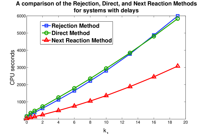
Figure 1: The above plot compares the speeds of the Rejection Method, Direct Method, and Next Reaction Method for systems with delays as the percentage of timesteps that are rejected in the Rejection Method, as parameterized by $k_{1}$, increases. For different values of $k_{1}$, each method was used to simulate the system (18) $10^{4}$ times. The plot above gives the CPU time needed for each method as a function of $k_{1}$. We see that the Rejection and Direct Methods are nearly equivalent while the Next Reaction Method for systems with delays is significantly more efficient than both for all $k_{1}$.

We see that as $k_{1}$ increases, the Rejection and Direct Methods remain relatively close in terms of efficiency with the Rejection Method being slightly more efficient for smaller $k_{1}$ and slightly less efficient for larger $k_{1}$. However, the Next Reaction Method for systems with delays (Algorithm 7), is significantly more efficient than both for all $k_{1}$.

VII Conclusion

By explicitly representing the reaction times of discrete stochastic chemical systems with the firing times of independent, unit rate Poisson processes with internal times given by integrated propensity functions we have developed a modified Next Reaction Method. We extended our modified Next Reaction Method to systems with delays and demonstrated its computational efficiency on such systems over the Rejection Method of Bratsun et al. and Barrio et al., and the Direct Method of Cai. Considering that many models of natural cellular processes such as gene transcription and translation have delays between the initiation and completion of reactions, and that the Rejection method appears to be the most widely used method for simulating such systems, we feel that this extension will be useful. Also, as is pointed out in the text, our modified Next Reaction Method can be easily extended to systems with non-exponential waiting times between initiations and is preferable to both the Gillespie Algorithm and the original Next Reaction Method for systems with propensities that depend explicitly on time. We feel that having a single, efficient simulation method applicable to such a broad range of chemical systems will prove to be a beneficial contribution.

Appendix A Unfinished calculation

In Section V we showed that if a system has propensity functions that depend explicitly on time, then the amount of absolute time, $\Delta$, that must pass after time $t$ before any reaction fires has distribution function

$$1-\exp\left(-\sum_{k=1}^{M}\int_{t}^{t+\Delta}a_{k}(X(t),s)ds\right).$$

where $r$ is uniform$(0,1)$. We will sketch the proof of why the reaction that fires at that time will be chosen according to the probabilities $a_{k}(X(t),t+\Delta)/a_{0}$, where $a_{0}=\sum_{k=1}^{M}a_{k}(X(t),t+\Delta)$.

Let $H(r)\ \dot{=}\ \sum_{k=1}^{M}\int_{t}^{t+r}a_{k}(X(t),s)ds.$ For $j\leq M$, let $\Delta t_{j}$ be the amount of time that must pass after time $t$ before the $j$th reaction fires. Let $F$ denote the random variable $\min\{\Delta t_{j}\}$. Then, conditioning on the fact that $F=\Delta$ and using the independence of the underlying Poisson processes we have

$$\begin{split}P(\Delta t_{k}<\Delta t_{j,j\neq k}|F=\Delta)&=\lim_{\delta\to 0}P(\Delta t_{k}<\Delta t_{j,j\neq k}|F\in[\Delta,\Delta+\delta))\\ &=\lim_{\delta\to 0}\frac{P(\Delta t_{k}<\Delta t_{j,j\neq k},F\in[\Delta,\Delta+\delta))}{P(F\in[\Delta,\Delta+\delta))}\\ &=\lim_{\delta\to 0}\frac{P(\Delta t_{k}\in[\Delta,\Delta+\delta),\Delta t_{j,j\neq k}>\Delta+\delta)}{\exp(-H(\Delta))-\exp(-H(\Delta+\delta))}\\ &=\lim_{\delta\to 0}\frac{P(\Delta t_{k}\in[\Delta,\Delta+\delta))\prod_{j\neq k}P(\Delta t_{j}>\Delta+\delta)}{\exp(-H(\Delta))-\exp(-H(\Delta+\delta))}.\end{split}$$ (20)

It is a simple exercise to show that for any $j\leq M$

$$P(\Delta t_{j}>s)=\exp\left(-\int_{t}^{t+s}a_{j}(X(t),s)ds\right).$$ (21)

Combining equations (20) and (21) with an application of L’Hopital’s rule gives the desired result.

Figures

Figure 1.

Captions

Caption for Figure 1.

The above plot compares the speeds of the Rejection Method, Direct Method, and Next Reaction Method for systems with delays as the percentage of timesteps that are rejected in the Rejection Method, as parameterized by $k_{1}$, increases. For different values of $k_{1}$, each method was used to simulate the system (18) $10^{4}$ times. The plot above gives the CPU time needed for each method as a function of $k_{1}$. We see that the Rejection and Direct Methods are nearly equivalent while the Next Reaction Method for systems with delays is significantly more efficient than both for all $k_{1}$.

References

- Arkin et al. 1998 A. Arkin, J. Ross, and H. H. McAdams, Genetics 149, 1633 (1998).
- McAdams and Arkin 1997 H. H. McAdams and A. Arkin, PNAS 94, 814 (1997).
- Ozbudak et al. 2002 E. M. Ozbudak, M. Thattai, I. Kurtser, A. D. Grossman, and A. van Oudenaarden, Nat. Genet. 31, 69 (2002).
- Samad et al. 2005 H. E. Samad, M. Khammash, L. Petzold, and D. Gillespie, Inter. J. Robust and Nonlinear Control 15, 691 (2005).
- Gillespie 1976 D. T. Gillespie, J. Comput. Phys. 22, 403 (1976).
- Gillespie 1977 D. T. Gillespie, J. Phys. Chem. 81, 2340 (1977).
- Gibson and Bruck 2000 M. Gibson and J. Bruck, J. Phys. Chem. A 105, 1876 (2000).
- Kurtz 1980 T. G. Kurtz, The Annals of Prob. 8, 682 (1980).
- Ethier and Kurtz 1986 S. N. Ethier and T. G. Kurtz, Markov Processes: Characterization and Convergence (John Wiley & Sons, New York, 1986).
- Ball et al. 2006 K. Ball, T. G. Kurtz, L. Popovic, and G. Rempala, Annals of Appl. Prob. 16, 1925 (2006).
- Bratsun et al. 2005 D. Bratsun, D. Volfson, L. S. Tsimring, and J. Hasty, PNAS 102, 14593 (2005).
- Barrio et al. 2006 M. Barrio, K. Burrage, A. Leier, and T. Tian, PLoS Comp. Biol. 2, 1017 (2006).
- Cai 2007 X. Cai, J. Chemical Physics 126, 124108 (2007).
- Burman 1981 D. Y. Burman, Adv. in Appl. Prob. 13, 846 (1981).
- Schassberger 1978 R. Schassberger, Advances in Appl. Prob. 10, 836 (1978).
- Glynn 1989 P. W. Glynn, Proc. of the IEEE 77, 14 (1989).
- Haas 2002 P. J. Haas, Stochastic Petri Nets: Modelling Stability, Simulation (Springer, New York, 2002), 1st ed.
- Anderson unpublshed D. F. Anderson (unpublshed).
- Rempala et al. 2006 G. A. Rempala, K. S. Ramos, and T. Kalbfleisch, J. Theor. Biol. 242, 101 (2006).