The typical behaviour of relays

Abstract

The typical behaviour of the relay-without-delay channel and its many-units generalisation, termed the relay array, under LDPC coding, is studied using methods of statistical mechanics. A demodulate-and-forward strategy is analytically solved using the replica symmetric ansatz which is exact in the studied system at the Nishimori’s temperature. In particular, the typical level of improvement in communication performance by relaying messages is shown in the case of small and large number of relay units.

I Introduction

Methods of statistical mechanics have recently become increasingly more important in the study of communication channels. The development of the replica and cavity methods for analysing disordered systems MPV ; Nishimori01 and the related recent introduction of systematic rigorous bounds Guerra03 ; Franz01 made new theoretical tools available for their analysis.

More specifically, the replica method has been applied to a wide range of problems in information theory, from error correcting codes Sourlas89 ; ksRev to multiuser communication Tanaka02 . It facilitates the derivation of practical and theoretical limits in various communication channels and provides typical results in cases that are difficult to tackle via traditional methods of information theory.

The growing use of information networks, both physically connected and wireless, and the increasing number of services taking place in the Internet, have made the study of multiuser communication highly attractive and relevant from a practical point of view, in addition to being a challenging and exciting field for theoretical research.

Up to date, there is no generalised theory of multiuser channels within the framework of information theory and analytical results are only known for special cases; the main difficulty being that multiuser networks do not admit the source-channel separation principle which plays an essential role in the analysis of communication channels. Nevertheless, multi-user communication plays an important role in a variety of communication devices ranging from mobile phones to computers. We strongly believe that a statistical physics-based analysis may offer answers where the current information theory methodology fails, especially in the limit of a large number of users.

With the technological demand and the possibility of a more thorough study by the methods of statistical mechanics, early results for multi-user communication are being revisited and analysed from different and complementary points of view, resulting in new insights and developments Tanaka02 ; NakamuraBroad . One of those interesting types of channels is the relay channel Cover91 . This generic channel is characterised by an auxiliary user between the transmitter and receiver, which helps in the transmission of the message. Due to the increase in the number of multi-user networks, like mobile phones and computer networks, the transfer of information with the help of a relays became an attractive option. As these networks are becoming more distributed, the transmission with the help of arrays of relays becomes feasible and merits further analytical exploration.

This paper is organised as follows. In section II we define the general relay array and introduce as particular cases the classical relay channel and the relay-without-delay. In section III we outline the statistical physics methods used to analyse the problem which will be based on a replica approach detailed in section IV. Section V contains our conclusions and final comments.

II The Model

II.1 LDPC Codes

Low-Density Parity-Check (LDPC) codes Gallager62 are state-of-the-art error-correcting codes with performance that is second to none, especially within the high code rate regime. In the notation we will be using here, $N$-dimensional messages ${\mathbf{s}}$ are encoded into $M$-dimensional codewords ${\mathbf{t}}$. LDPC codes are defined by a binary parity-check matrix $A=[C_{1}\mid C_{2}]$, concatenating two very sparse matrices known to both sender and receiver: $C_{2}$ that is invertible and of dimensionality $(M-N)\times(M-N)$ and $C_{1}$ of dimensionality $(M-N)\times N$. The matrix $A$ can be either random or regular, characterised by the number of non-zero elements per row ($K$) and column ($C$). Irregular codes show superior performance to regular structures Richardson01 ; idosaad1 if constructed carefully. In order to simplify our treatment, we focus here on regular constructions; the generalisation to irregular codes is straightforward Vicente02 ; VSK .

Encoding refers to the linear mapping of a $N$-dimensional original message ${\mathbf{s}}\in\{0,1\}^{N}$ to a $M$-dimensional codeword ${\mathbf{t}}\in\{0,1\}^{M}$ ($M>N$)

$${\mathbf{t}}=G{\mathbf{s}}\ \ \mbox{(mod 2)}\ ,$$ (1)

where all operations are performed in the field $\{0,1\}$ and are indicated by (mod 2). The generator matrix is

$$G={\left(\begin{array}[]{c}I\\ C_{2}^{-1}C_{1}\end{array}\right)}\ \ \mbox{(mod 2)}\ ,$$ (2)

where $I$ is the $N\times N$ identity matrix. By construction $AG=0\ \mbox{ (mod 2)}$ and the first $N$ bits of ${\mathbf{t}}$ correspond to the original message ${\mathbf{s}}$.

Decoding is carried out by estimating the most probable transmitted vector from the received corrupted codeword Vicente02 ; ksRev . For mathematical convenience, in the present work we map the Boolean variable ${\mathbf{t}}\in\{0,1\}^{M}$ into a spin variable ${\mathbf{t}}\in\{1,-1\}^{M}$ by the transformation $x\rightarrow(-1)^{x}$.

II.2 The Relay Array

The relay array is a many-units generalisation of the (single unit) relay channel of Cover91 . The LDPC codeword ${\mathbf{t}}$ is transmitted to each one of $L$ relay units through noise channels corrupted by a global Additive White Gaussian Noise (AWGN) $\mbox{\boldmath{$\nu$}}_{0}$ and by local independent AWGNs $\mbox{\boldmath{$\nu$}}_{i}$. Each relay processes the received corrupted message ${\mathbf{r}}_{i}$ and encodes the acquired information into a vector ${\mathbf{t}}_{i}$ which is then transmitted to a final receiver. The final receiver receives an algebraic summation of the relay outputs plus a direct transmission from the original sender, corrupted also by $\mbox{\boldmath{$\nu$}}_{0}$, subject to a final AWGN $\nu$. The exact form of the channel is depicted in Fig. 1 and the corresponding equations are

$${\mathbf{r}} =a{\mathbf{t}}+\sum_{i=1}^{L}b_{i}{\mathbf{t}}_{i}+\mbox{\boldmath{$\nu$}}+\mbox{\boldmath{$\nu$}}_{0},$$ (3)

$${\mathbf{r}}_{i} =c_{i}{\mathbf{t}}+\mbox{\boldmath{$\nu$}}_{i}+\mbox{\boldmath{$\nu$}}_{0}.$$ (4)

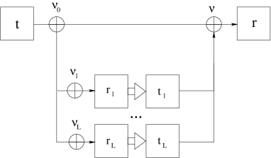
Figure 1: The $L$-component relay array. The original sender sends a codeword ${\mathbf{t}}$ to the final receiver and to each of the $L$ relays. Each relay receives a message ${\mathbf{r}}_{i}$ which is a corrupted version of the original codeword subject to the AWGNs $\mbox{\boldmath{$\nu$}}_{0}$ and $\mbox{\boldmath{$\nu$}}_{i}$. It then sends to the final receiver the encoded vector ${\mathbf{t}}_{i}$. The final receiver receives the original transmitted codeword summed with all ${\mathbf{t}}_{i}$’s and corrupted by the AWGN vectors $\mbox{\boldmath{$\nu$}}_{0}$ and $\nu$.

The variables $a$, $b_{i}$ and $c_{i}$ ($i=1,...,L$) are the relative gains of each transmission and can be random or set to constant values. The power from the original source to each relay is $c_{i}^{2}$, to the final receiver is $a^{2}$ and the power from each relay to the final receiver is $b_{i}^{2}$.

When $L=1$, we refer to the channel simply as the relay channel. In the classical relay channel (CRC), studied by Cover and El-Gamal Cover79 , the messages sent by the relays to the final receiver are only allowed to depend on the set of symbols received by the each of the relays before the current time step, $t_{i}^{\mu}=f(t^{1},...,t^{\mu-1})$, which corresponds to the fact that it takes the relay some time to process the information before relaying it. However, if the time delay in the direct transmission to the final receiver is much longer than in the transmission to the relay units, we can allow the message sent by the relay to depend on the present received symbol as well such that $t_{i}^{\mu}=f(t^{1},...,t^{\mu})$. This last case, termed relay-without-delay (RWD), created significant interest recently and was studied by El-Gamal and Hassanpour ElGamal05 . For the case of a relay array where all communication is carried out through the relays and there is no direct transmission to the final receiver, the restriction of the CRC, to consider all but the last received symbol, is unnecessary.

III Statistical Physics of Decoding

We transform the decoding problem of the final receiver into a statistical physics system by defining a dynamical variable $\mbox{\boldmath{$\tau$}}\equiv(\tau^{1},...,\tau^{M})$ which represents the candidate variable vectors at the receiver. Each $\tau^{\mu}$ plays a role equivalent to a spin located in the $\mu$-th site of a lattice with $M$ sites.

The final receiver generates an estimate $\hat{{\mathbf{t}}}$ of the original codeword using the Marginal Posterior Maximiser (MPM) estimator

$$\hat{t}^{\mu}={\mbox{sgn}\,}{\left<\tau^{\mu}\right>_{{\mathcal{P}{\left(\mbox{\boldmath{$\tau$}}|{\mathbf{r}}\right)}}}},$$ (5)

which minimises the probability of bit error Iba99 ; Vicente02 . Other estimators can be used depending on the error measure considered. For example, minimisation of block error is obtained using the Maximum a Posteriori (MAP) estimator.

The posterior probability density is calculated by Bayes’ rule as

$${\mathcal{P}{\left(\mbox{\boldmath{$\tau$}}|{\mathbf{r}}\right)}}=\frac{{\mathcal{P}{\left({\mathbf{r}}|\mbox{\boldmath{$\tau$}}\right)}}{\mathcal{P}{\left(\mbox{\boldmath{$\tau$}}\right)}}}{{\mathcal{P}{\left({\mathbf{r}}\right)}}},$$ (6)

with

$${\mathcal{P}{\left({\mathbf{r}}\right)}} =\sum_{{\mathbf{t}}}{\mathcal{P}{\left({\mathbf{r}}|{\mathbf{t}}\right)}}{\mathcal{P}{\left({\mathbf{t}}\right)}}$$

$$=\sum_{{\mathbf{t}},{\left\{{\mathbf{t}}_{i}\right\}},{\left\{{\mathbf{r}}_{i}\right\}}}{\mathcal{P}{\left({\mathbf{t}}\right)}}{\mathcal{P}{\left({\mathbf{r}}|{\mathbf{t}},{\left\{{\mathbf{t}}_{i}\right\}}\right)}}\prod_{i}{\mathcal{P}{\left({\mathbf{t}}_{i}|{\mathbf{r}}_{i}\right)}}{\mathcal{P}{\left({\mathbf{r}}_{i}|{\mathbf{t}}\right)}}.$$ (7)

One of the basic quantities of interest is the overlap between the codeword and the decoded message. Our analysis, focuses on the typical behaviour of the decoding process and, accordingly, we take averages over all possible codewords, all received messages and all allowed encodings, which we consider as quenched disorder in the system. The overlap between decoded and original message takes the form

$$d=\frac{1}{M}\sum_{\mu=1}^{M}{\left<t^{\mu}\,{\mbox{sgn}\,}{\left<\tau^{\mu}\right>_{{\mathcal{P}{\left(\mbox{\boldmath{$\tau$}}|\mbox{\boldmath{$r$}}\right)}}}}\right>_{{A,{\mathbf{r}},{\mathbf{t}}}}}.$$ (8)

This quantity can be derived from the free-energy

$$f=-\lim_{M\rightarrow\infty}\frac{1}{\beta M}{\left<\ln Z\right>_{{A,{\mathbf{r}},{\mathbf{t}}}}},$$ (9)

with the partition function

$$Z=\sum_{{\mathbf{t}}}e^{-\beta\mathcal{H}{\left({\mathbf{t}};{\mathbf{r}}\right)}},$$ (10)

and the corresponding Hamiltonian

$$\mathcal{H}{\left({\mathbf{t}};{\mathbf{r}}\right)}=-\ln{\mathcal{P}{\left({\mathbf{r}}|{\mathbf{t}}\right)}}{\mathcal{P}{\left({\mathbf{t}}\right)}}.$$ (11)

Usually we disregard the normalisation of the distributions within the Hamiltonian as they merely add constants that shift the zero energy. In the case of LDPC codes, ${\mathcal{P}{\left({\mathbf{t}}\right)}}$ turns out to be a constraint on the summation variables.

In the above Hamiltonian, the parity-check matrix $A$ defines an interaction between the $\tau$ variables while ${\mathbf{t}}$ and ${\mathbf{r}}$ act as local fields. The inverse temperature $\beta$ is the ratio between the true and the decoder’s assumed noise level. In our numerical calculations, we adopt $\beta=1$, also known as Nishimori’s temperature, which means that the decoder assumes the correct noise level for the channel. It can be shown that at Nishimori’s temperature the system never enters the glassy phase Nishimori01 ; Montanari01 and the thermodynamically dominant solution is always Replica Symmetric (RS); we therefore restrict our analysis to the RS treatment.

One of the important properties and the novelty of the statistical physics formulation of the problem is that looking at the problem as a dynamical spin system, we can interpret the results in terms of phase transitions which can be characterised by the overlap and the entropy function. Combining this extra information we can have a better understanding of the way the system changes from a phase of perfect decoding (which is called the ferromagnetic phase) to a phase where the message is recovered only up to a certain amount of error (the paramagnetic phase).

The most studied strategies used by the relay units are the Amplify-and-Forward (A&F) and the Decode-and-Forward (D&F) strategies. In A&F, the relay just retransmits its received vector, i.e., ${\mathbf{t}}_{i}={\mathbf{r}}_{i}$. As the replica treatment of this case turns out to be the same as for the simple Gaussian channel with a modified power and noise level, the solution is obtained straightforwardly by applying the results of Vicente02 and will not be studied here.

In the D&F strategy, the relays decode the message and transmit their estimate to the final receiver. Full use of LDPC decoding in the relays is made when each relay decodes the received vector ${\mathbf{r}}_{i}$ by the MPM estimator using the fact that the codeword was encoded by an LDPC code. The message transmitted to the final receiver by each relay would then be

$$t_{i}^{\mu}={\mbox{sgn}\,}{\left<\tau_{i}^{\mu}\right>_{{\mathcal{P}{\left(\mbox{\boldmath{$\tau$}}_{i}|{\mathbf{r}}_{i}\right)}}}}.$$ (12)

In equation (6) this is equivalent to setting

$${\mathcal{P}{\left({\mathbf{t}}_{i}|{\mathbf{r}}_{i}\right)}}=\prod_{\mu=1}^{M}\delta{\left(t_{i}^{\mu}-{\mbox{sgn}\,}{\left<\tau_{i}^{\mu}\right>_{{\mathcal{P}{\left(\mbox{\boldmath{$\tau$}}_{i}|{\mathbf{r}}_{i}\right)}}}}\right)}.$$ (13)

As $t_{i}^{\mu}\in\{\pm 1\}$, we can rewrite this probability density as

$${\mathcal{P}{\left({\mathbf{t}}_{i}|{\mathbf{r}}_{i}\right)}}=\prod_{\mu=1}^{M}\theta{\left({\left<t_{i}^{\mu}\tau_{i}^{\mu}\right>_{{\mathcal{P}{\left(\mbox{\boldmath{$\tau$}}_{i}|{\mathbf{r}}_{i}\right)}}}}\right)},$$ (14)

where $\theta$ is the Heaviside step function.

The replica treatment of the LDPC D&F turns out to be extremely involved due to the introduction of a theta function with an average over the variables $\mbox{\boldmath{$\tau$}}_{i}$ inside it, which includes a term dependant on the parity-check matrix. Analytical studies in order to solve this, rather difficult case, are under way.

In the present work we focus on a simplification of this strategy also known in the literature as Demodulate-and-Forward. In it case, the relays do not have the complete information about the encoding mechanism and therefore assume a uniform prior for the transmitted codeword. In this case, the posterior distribution of the bits in the message for the relay is

$${\mathcal{P}{\left({\mathbf{t}}_{i}|{\mathbf{r}}_{i}\right)}}=\prod_{\mu=1}^{M}\frac{1}{1+\exp{\left[-2t_{i}^{\mu}r_{i}^{\mu}/(\sigma_{i}^{2}+\sigma_{0}^{2})\right]}},$$ (15)

and it is straightforward to show that the MPM estimator is given simply by

$$t_{i}^{\mu}={\mbox{sgn}\,}{\left(r_{i}^{\mu}\right)}.$$ (16)

The fact that the disorder relative to different codes does not appear in the estimate of the relays makes the replica calculations feasible in this case, as follows.

IV Replica Symmetric Analysis

As the RS analysis of LDPC coding systems has been introduced and carried out in a number of publications (e.g.  Vicente02 ) we will skip the detailed derivation and concentrate on the final expressions. The derivation follows exactly the same steps as in Alamino07 where quenched averages are first carried out, followed by the RS assumption which enables the representation of the order parameters in the form of field distributions. These are obtained using a set of self-consistent saddle point equations of the form

$${\hat{\pi}}({\hat{x}}) ={\left<\delta{\left({\hat{x}}-\prod_{m=1}^{K-1}x^{m}\right)}\right>_{{\mathbf{x}}}},$$ (17)

$$\pi(x) ={\left<\delta{\left(x-\frac{\sum_{\tau}\tau\,{\left[\Psi(\tau,r)\right]}^{\beta}\prod_{l=1}^{C-1}{\left(1+\tau{\hat{x}}^{l}\right)}}{\sum_{\tau}{\left[\Psi(\tau,r)\right]}^{\beta}\prod_{l=1}^{C-1}{\left(1+\tau{\hat{x}}^{l}\right)}}\right)}\right>_{r,{\mathbf{{\hat{x}}}}}},$$

where

$$\Psi(\tau,r) \equiv\int{\left\{\prod_{i=1}^{L}dr_{i}\,\exp{\left[-\frac{{\left(r_{i}-c_{i}\tau\right)}^{2}}{2(\sigma_{i}^{2}+\sigma_{0}^{2})}\right]}\right\}}$$

$$\times\exp{\left[-\frac{1}{2(\sigma^{2}+\sigma_{0}^{2})}{\left(r-a\tau-\sum_{i}b_{i}\,{\mbox{sgn}\,}r_{i}\right)}^{2}\right]}.$$ (18)

The expression ${\left<t_{i}\right>}$ is the mean of the variable $t_{i}$ and ${\mathcal{P}{\left(r\right)}}\propto\Psi(1,r)$. The overlap is

$$d ={\left<{\mbox{sgn}\,}u\right>_{u}},~{}\mbox{with}$$ (19)

$${\mathcal{P}{\left(u\right)}} ={\left<\delta{\left(u-\frac{\sum_{\tau}\tau\,{\left[\Psi(\tau,r)\right]}^{\beta}\prod_{l=1}^{C}{\left(1+\tau{\hat{x}}^{l}\right)}}{\sum_{\tau}{\left[\Psi(\tau,r)\right]}^{\beta}\prod_{l=1}^{C}{\left(1+\tau{\hat{x}}^{l}\right)}}\right)}\right>_{r,{\mathbf{{\hat{x}}}}}},$$ (20)

the free energy is given by

$$\beta f =\frac{C}{K}\ln 2+C{\left<\ln(1+x{\hat{x}})\right>_{x,{\hat{x}}}}$$

$$-\frac{C}{K}{\left<\ln{\left(1+\prod_{m=1}^{K}x^{m}\right)}\right>_{{\mathbf{x}}}}$$

$$-{\left<\ln{\left\{\sum_{\tau}{\left[\Psi(\tau,r)\right]}^{\beta}\prod_{l=1}^{C}{\left(1+\tau{\hat{x}}^{l}\right)}\right\}}\right>_{{\mathbf{{\hat{x}}}},r}},$$ (21)

and the internal energy, the derivative with respect to $\beta$ of the above equation, is

$$u =-{\left<\frac{\sum_{\tau}\Psi^{\beta}(\ln\Psi)\prod_{l=1}^{C}{\left(1+\tau{\hat{x}}^{l}\right)}}{\sum_{\tau}\Psi^{\beta}\prod_{l=1}^{C}{\left(1+\tau{\hat{x}}^{l}\right)}}\right>_{{\mathbf{{\hat{x}}}},r}}.$$ (22)

For any number $L$ of relays, the results can be obtained by a numerical solution of the equations (17). Note the summation over the internal variables, i.e., the messages received and sent by the relays. This comes from the Bayesian formulation of the problem where the final receiver has access just to ${\mathbf{r}}$ and, therefore, must integrate over the unknown variables.

We also note that the above equations are fairly general. Using the appropriate “potential” $\Psi$ we can recover all previous results for single user channels and apply them to more general channels when the intermediate processing of the message does not involve the previous knowledge of the parity-check matrices.

The ferromagnetic state, which corresponds to perfect decoding, is given by the following solution to the saddle point equations (17)

$${\hat{\pi}}({\hat{x}})=\delta({\hat{x}}-1),\qquad\pi(x)=\delta(x-1).$$ (23)

Substitution of these distributions in equation (19) gives $d=1$. By substituting the ferromagnetic solution into the formulas for the free and internal energies, we obtain (for Nishimori’s temperature)

$$u=f=-{\left<\ln\Psi(1,r)\right>_{r}},$$ (24)

meaning that the entropy of this phase is zero.

The Hamiltonian of the relay array is gauge invariant with respect to the gauge transformation

$$r^{\mu} \rightarrow\gamma^{\mu}r^{\mu},$$

$$t^{\mu} \rightarrow\gamma^{\mu}t^{\mu},$$ (25)

where the vector $\gamma$ obeys the parity-check constraints. We can verify that the transition probabilities ${\mathcal{P}{\left(r^{\mu}|t^{\mu}\right)}}$ are also invariant under this gauge transformation. Note that if a channel is symmetric (for a definition see Tanaka03 ), it is automatically gauge invariant under the above transformation. For gauge invariant channels the internal energy is

$$U ={\left<\mathcal{H}{\left(\mbox{\boldmath{$\tau$}};{\mathbf{r}}\right)}\right>_{\mbox{\boldmath{$\tau$}},{\mathbf{r}},{\mathbf{t}}}}$$

$$=\sum_{\mbox{\boldmath{$\tau$}},{\mathbf{t}}}\int d{\mathbf{r}}\,{\mathcal{P}{\left(\mbox{\boldmath{$\tau$}}|{\mathbf{r}},\beta\right)}}{\mathcal{P}{\left({\mathbf{r}}|{\mathbf{t}}\right)}}{\mathcal{P}{\left({\mathbf{t}}\right)}}\mathcal{H}{\left(\mbox{\boldmath{$\tau$}};{\mathbf{r}}\right)},$$ (26)

where

$${\mathcal{P}{\left(\mbox{\boldmath{$\tau$}}|{\mathbf{r}},\beta\right)}}\propto e^{-\beta\mathcal{H}},$$ (27)

is the thermal Gibbs probability at inverse temperature $\beta$ which obeys ${\mathcal{P}{\left(\mbox{\boldmath{$\tau$}}|{\mathbf{r}},\beta=1\right)}}={\mathcal{P}{\left(\mbox{\boldmath{$\tau$}}|{\mathbf{r}}\right)}}$. Since under such a gauge transformation the Hamiltonian remains invariant, we have $\mathcal{H}{\left({\mathbf{t}};{\mathbf{r}}\right)}=\mathcal{H}{\left({\mathbf{1}};{\mathbf{t}}{\mathbf{r}}\right)}$, where ${\mathbf{t}}{\mathbf{r}}\equiv(t^{1}r^{1},...,t^{M}r^{M})$ and ${\mathbf{1}}$ is an $M$-dimensional vector with all entries equal to 1. Therefore, one can write

$$U=\sum_{\mbox{\boldmath{$\tau$}},{\mathbf{t}}}\int d{\mathbf{r}}\,\frac{{\mathcal{P}{\left({\mathbf{r}}|\mbox{\boldmath{$\tau$}},\beta\right)}}{\mathcal{P}{\left(\mbox{\boldmath{$\tau$}}|\beta\right)}}}{{\mathcal{P}{\left({\mathbf{r}}|\beta\right)}}}{\mathcal{P}{\left({\mathbf{r}}|{\mathbf{t}}\right)}}{\mathcal{P}{\left({\mathbf{t}}\right)}}\mathcal{H}{\left({\mathbf{1}};\mbox{\boldmath{$\tau$}}{\mathbf{r}}\right)}.$$ (28)

Gauging the variables $\mbox{\boldmath{$\tau$}}{\mathbf{r}}\rightarrow{\mathbf{r}}$, reorganising the terms and taking $\beta=1$, we finally get

$$U=\int d{\mathbf{r}}\,{\mathcal{P}{\left({\mathbf{r}}|{\mathbf{1}}\right)}}\mathcal{H}{\left({\mathbf{1}};{\mathbf{r}}\right)}.$$ (29)

The meaning of this is that, for a gauge invariant channel of the type described above (which includes the symmetric channels), the internal energy is independent of the configuration. In special cases, as can be found in Nishimori01 , the gauge symmetry allows an analytical expression to be found. The same method can be used to prove that the probability distribution for the magnetisation is equal to the probability distribution for the two-point correlations in Nishimori’s temperature, which indicates the absence of a spin glass phase and no replica symmetry breaking.

IV.1 The Relay Channel

In order to compare our results with those of ElGamal05 , we analyse the RWD for the setup sketched in Fig. 2 with $\sigma_{1}^{2}=\eta\sigma^{2}$, $a=b_{1}=1$ and $c_{1}=(1+\sigma^{2})^{-1/2}$. The potential is then given by

$$\Psi(\tau,r) =e^{-{\left(r-\tau-1\right)}^{2}/2\sigma^{2}}\,{\mbox{erfc}\,}{\left(-\frac{\tau}{\sqrt{2\eta\sigma^{2}}}\right)}$$

$$+e^{-{\left(r-\tau+1\right)}^{2}/2\sigma^{2}}\,{\mbox{erfc}\,}{\left(+\frac{\tau}{\sqrt{2\eta\sigma^{2}}}\right)},$$ (30)

where ${\mbox{erfc}\,}(x)$ is the complementary error function

$${\mbox{erfc}\,}(x)=\frac{2}{\sqrt{\pi}}\int_{x}^{\infty}e^{-y^{2}}\,dy.$$ (31)

Figure 2: Schematic drawing of the relay-without-delay (RWD) setup to be analysed.

For these values of noise and gains, the capacity of this channel as derived in ElGamal05 is

$$\mathcal{C}=\frac{1}{2}\log_{2}{\left(1+\frac{1+c_{1}^{2}}{\sigma^{2}}\right)}.$$ (32)

The numerical results for the overlap between the retrieved and the original codewords, obtained by solving recursively equations (17), are given in Fig. 3 for $K=4$, $C=3$, $\beta=1$ and $\eta=0.1$. Shannon’s limit is indicated by the vertical dashed line and corresponds to a noise level $\sigma^{2}\approx 8.79$. The dashed curve shows the overlap for a simple Gaussian channel with noise level $\sigma^{2}$ and the continuous one shows the overlap for the RWD. The improvement in the practical limit for error-free communication, indicated by the highest noise level for which $d=1$ is clear. However, the distance between the dynamical transition threshold $\sigma_{d}^{2}\approx 2.22$ and Shannon’s limit for the channel is greater than in the case of the simple Gaussian channel (for numerical results for the Gaussian channel see Tanaka03 ). Numerical calculations point to the expected result that decreasing the noise level from the source to the relay brings $\sigma_{d}^{2}$ closer to Shannon’s limit. However, one must remember that the relay strategy examined does not use the full potential of the relay and the additional information embedded in the LDPC codes. We expect that a LDPC decoding in the relay will improve the communication performance and currently focus on the analysis of this scenario.

We can also see in the plot that, as the noise level increases, the channel becomes closer to the Gaussian channel. This is just a consequence of the fact that, for high noise level, the additional information provided by the relay becomes negligible as both users decode the message poorly.

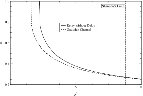
Figure 3: The overlap of retrieved and original codewords for the RWD channel with $\sigma_{1}^{2}=0.1\sigma^{2}$ is given by the continuous curve. The dashed curve shows the same for the simple Gaussian channel. The vertical line indicate Shannon’s limit for the RWD as calculated by El-Gamal and Hassanpour ElGamal05 .

Figure 4 shows the entropy and the free and internal energies for the same values as in Fig. 3. At the dynamical transition point, where practical perfect decoding becomes unfeasible, the entropy becomes negative, indicating the emergence of subdominant metastable states that can be further explored using the replica symmetry breaking ansatz. Between this point and the thermodynamical transition point, where the entropy is positive again, the dominant state is still ferromagnetic but the population dynamics algorithm used to solve the saddle point equations becomes trapped in a local minimum with free-energy higher than the ferromagnetic one. Due to the equality between the internal energy and the ferromagnetic free-energy, the point where the entropy becomes positive again is also the point where both energies cross in the bottom graph.

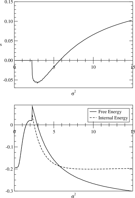
Figure 4: Entropy and energies for the RWD channel at Nishimori’s temperature. The upper graph shows the entropy which is given by the difference between the internal energy and the free energy depicted in the bottom graph.

In Fig. 5 we plot the dynamical and thermodynamical transition noise levels against $\eta$, the ratio between the relay and final receiver noise levels. We see that the dynamical and thermodynamical transition points decrease with $\eta$ but became closer to each other, stabilising at asymptotic values that match those of the simple AWGN channel values as the relay contribution becomes meaningless.

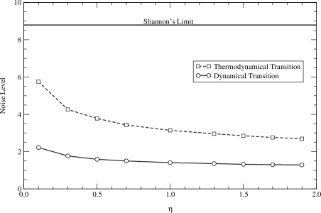
Figure 5: The continuous/dashed line shows the dynamical/thermodynamical transition noise levels of the RWD against $\eta$, the ratio between relay and final receiver noise levels. The upper horizontal line corresponds to Shannon’s limit $\sigma^{2}\approx 8.79$.

Although the capacity for the RWD is known only in special cases, its upper bound can be higher than in the case of the CRC. In order to verify it for the LDPC-based framework we analyse in this paper, we now use a setup equivalent to the one studied in Cover79 and shown in Fig. 6 where $a=c_{1}=b_{1}=1$ and $\sigma_{0}^{2}\equiv\lambda\sigma^{2}$. The capacity of the CRC in this case is

$$\mathcal{C}=\left\{\begin{array}[]{cc}\frac{1}{2}\log_{2}{\left(1+\frac{1}{\lambda\sigma^{2}}\right)},&\lambda\geq 1,\\ &\\ \frac{1}{2}\log_{2}{\left(1+\frac{4}{(1+\lambda)^{2}\sigma^{2}}\right)},&\lambda<1.\end{array}\right.$$ (33)

Figure 6: Schematic drawing of the classical relay channel (CRC) setup. The relative gains are all equal to 1 and not shown in the picture.

In Fig. 7 we compare the dynamical and thermodynamical threshold noise levels of a RWD with Shannon’s limit for the CRC, both with the setup described above, for different values of $\lambda$, the ratio between the noise levels applied at the transmission and reception points.

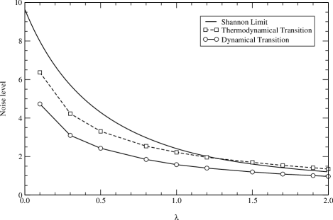
Figure 7: The continuous/dashed line shows the dynamical/thermodynamical transition noise levels of the RWD against $\lambda$ in the setup of Fig. 6. The continuous line without marked symbols is Shannon’s limit for a CRC with the same noise levels and transmission powers.

We can see that, although the practical decoding line (dynamical transition) falls below Shannon’s limit for all calculated values, the thermodynamical transition goes above it for the CRC case at higher values of $\lambda$. Figure 7 shows that the capacity of the RWD is indeed higher than the CRC for the case studied and quantifies the gain in allowing the message sent by the relay to depend on the current transmitted symbol (which is excluded in the CRC). Although allowing this instantaneous dependence would at first sight seem just a small modification which is insignificant in the infinite block length limit, it indeed gives relevant extra information which facilitates more efficient retrieval at the final receiver. The insight gained is that for the RWD and large $\lambda$, the relay transmission $t_{1}^{\mu}$ is correlated with the original codeword $t^{\mu}$, which is not the case in the CRC allows; this allows for an improvement in the information extraction at the receiver.

IV.2 Large Relay Array

Now, we will use the central limit theorem to obtain the result for large $L$ in the relay array setup given by Fig. 1. As the relay messages are correlated and to guarantee that the quantities have the same order, we introduce a $1/L$ scaling in the summation over relay messages. The potential for this model becomes

$$\Psi(\tau,r)\equiv\int{\left\{\prod_{i=1}^{L}dr_{i}\,\exp{\left[-\frac{{\left(r_{i}-\tau\right)}^{2}}{2(\sigma_{i}^{2}+\sigma_{0}^{2})}\right]}\right\}}$$

$$\times\exp{\left[-\frac{1}{2(\sigma^{2}+\sigma_{0}^{2})}{\left(r-\tau-\frac{1}{L}\sum_{i}{\mbox{sgn}\,}r_{i}\right)}^{2}\right]},$$ (34)

where we assumed, for simplicity, $a=b_{i}=c_{i}=1$.

For $L\gg 1$, the central limit theorem amounts to a modification in the distribution of the variable $r$ given by

$${\mathcal{P}{\left(r\right)}}=\int{\left[\prod_{i=1}^{L}dr_{i}\,{\mathcal{P}{\left(r_{i}\right)}}\right]}F{\left(\frac{1}{L}\sum_{i=1}^{L}{\mbox{sgn}\,}r_{i}\right)}={\left<F(\omega)\right>_{\omega}},$$ (35)

where

$$F(\omega) =\frac{1}{\sqrt{2\pi\sigma^{2}}}\exp{\left[-\frac{{\left(r-1-\omega\right)}^{2}}{2(\sigma^{2}+\sigma_{0}^{2})}\right]},$$ (36)

$${\mathcal{P}{\left(r_{i}\right)}} =\frac{1}{\sqrt{2\pi\sigma_{i}^{2}}}\,\exp{\left[-\frac{{\left(r_{i}-1\right)}^{2}}{2(\sigma_{i}^{2}+\sigma_{0}^{2})}\right]},$$ (37)

with

$${\mathcal{P}{\left(\omega\right)}}={\mathcal{N}{\left(\frac{1}{L}\sum_{i=1}^{L}{\left<{\mbox{sgn}\,}r_{i}\right>_{r_{i}}},\frac{1}{L^{2}}\sum_{i=1}^{L}{\left(1-{\left<{\mbox{sgn}\,}r_{i}\right>_{r_{i}}}\right)}^{2}\right)}}.$$ (39)

For simplicity, we consider the case where the noise level is the same for all relays $\sigma_{i}^{2}=\sigma_{1}^{2}$ and define

$$\sigma_{r}^{2}\equiv\sigma^{2}_{1}+\sigma_{0}^{2},\qquad\sigma_{f}^{2}\equiv\sigma^{2}+\sigma_{0}^{2}.$$ (40)

Then the corresponding distribution for $\omega$

$${\mathcal{P}{\left(\omega\right)}}={\mathcal{N}{\left({\mbox{erf}\,}{\left(1/\sqrt{2}\sigma_{r}\right)},\frac{1}{L}\,{\mbox{erfc}\,}^{2}{\left(1/\sqrt{2}\sigma_{r}\right)}\right)}}.$$ (41)

Consequently the contribution for the final noise level coming from the relay transmission decreases as $L^{-1}$. In the limit $L\rightarrow\infty$, this distribution becomes a delta function centred at the error function and therefore

$${\mathcal{P}{\left(r\right)}}={\mathcal{N}{\left(1+{\mbox{erf}\,}{\left(1/\sqrt{2}\sigma_{r}\right)},\sigma_{f}^{2}\right)}}.$$ (42)

Accordingly, the potential becomes

$$\Psi(\tau,r)=\exp{\left\{-\frac{1}{2\sigma_{f}^{2}}{\left[r-\tau-{\mbox{erf}\,}{\left(\tau/\sqrt{2}\sigma_{r}\right)}\right]}^{2}\right\}}.$$ (43)

Figure 8 compares the dynamical and thermodynamical transition points for $L=1,2,3,4,5$ calculated by the exact formula and the result obtained by the approximation for large $L$. Again, we consider the case of $K=4$, $C=3$ and $\beta=1$.

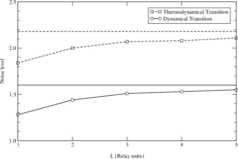
Figure 8: Dynamical and thermodynamical transition points for many relays. The exact formula is used to calculate the points $L=1,2,3,4,5$. The horizontal lines represent the large $L$ limit.

It is clear from Fig. 8 that already at $L=5$, both dynamical and thermodynamical transition points approach the large $L$ limit solution, thus making this approximation attractive already for low $L$ values.

V Conclusions

In this work we analysed the behaviour of relay arrays using methods of statistical mechanics. These networks are of growing significance due to the increase of multi-user, mobile and distributed communication systems.

We found an analytical solution for the relay-without-delay (RWD) channel given by the RS ansatz, which due to the gauge symmetry of the channel, is exact at Nishimori’s temperature that correspond to a choice of the correct prior within the Bayesian framework. We showed the level of improvement with respect to a simple Gaussian channel without relaying which, even for the naive relay strategy of Demodulate-and-Forward analysed here, is significant.

We compared the RWD dynamical and thermodynamical transition points for different noise ratios between the relay and the direct channel; and found that although these points become far from Shannon’s limit, the difference between the dynamical and the thermodynamical transition decreases. The relevance of the relay is clearly decreasing as its noise level increases as the level of additional information it conveys diminishes.

We also were able to compare the RWD case to the classical relay channel (CRC) for different noise ratios between the relay and the direct channel. We found that the capacity of the RWD is higher than the CRC for a high relay noise, showing the significance of the extra information conveyed by the relay on the current transmitted symbol, which is absent in the CRC framework.

The performance of a large array of relays was analysed and compared against results obtained for a small number of units. The result obtained are consistent and indicate that this useful approximation provides accurate results already for a small number of units. For a large array, we also found that the increase in noise tolerance levels off.

We have demonstrated the usefulness of methods adopted from statistical physics for analysing multi-user communication systems. While we have concentrated on limited scenarios of relay channels, we believe that these methods hold a promising alternative to the information theory methodology which, in general, has not been successful in dealing with multi-user communication systems. The study of different relay channels and other multi-user communication networks is underway.

References

- (1) M. Mézard, G. Parisi, and M. Virasoro, Spin Glass Theory and Beyond (World Scientific Publishing Co., Singapore, 1987).
- (2) H. Nishimori, Statistical Physics of Spin Glasses and Information Processing (Oxford University Press, Oxford, UK, 2001).
- (3) F. Guerra, Commun. Math. Phys. 233, 1 (2003).
- (4) S. Franz, M. Leone, F. Ricci-Tersenghi, and R. Zecchina, Phys. Rev. Lett. 87, 127209 (2001).
- (5) N. Sourlas, Nature 339, 693 (1989).
- (6) Y. Kabashima and D. Saad, J. Phys. A. 37, R1 (2004).
- (7) T. Tanaka, IEEE Trans. Inf. Theory 11, 2888 (2002).
- (8) K. Nakamura, Y. Kabashima, R. Morelos-Zaragoza, and D. Saad, Phys. Rev. E 67, 036703 (2003).
- (9) T. M. Cover and J. Thomas, Elements of Information Theory (John Wiley & Sons, New York, NY, 1991).
- (10) R. Gallager, IRE Trans. Inf. Theory IT-8, 21 (1962).
- (11) T. Richardson, A. Shokrollahi, and R. Urbanke, IEEE Trans. Inf. Theory 47, 619 (2001).
- (12) I. Kanter and D. Saad, Phys. Rev. Lett. 83, 2660 (1999).
- (13) R. Vicente, D. Saad, and Y. Kabashima, in Advances in Imaging and Electron Physics, edited by P. Hawkes (Academic Press, ADDRESS, 2002), Vol. 125, pp. 232–353.
- (14) R. Vicente, D. Saad, and Y. Kabashima, J. Phys. A 33, 6527 (2000).
- (15) T. M. Cover and A. A. El-Gamal, IEEE Trans. Inf. Theory 25, 572 (1979).
- (16) A. El-Gamal and N. Hassanpour, Proc. Int. Symposium on Inf. Theory, ISIT 2005 1078 (2005).
- (17) Y. Iba, J. Phys. A 32, 3875 (1999).
- (18) A. Montanari, Eur. Phys. J. B 23, 121 (2001).
- (19) R. C. Alamino and D. Saad, Preprint 1 (2007).
- (20) T. Tanaka and D. Saad, J. Phys. A 36, 11143 (2003).