Coarse Grained Density Functional Theories for Metallic Alloys: Generalized Coherent Potential Approximations and Charge Excess Functional Theory.

Abstract

The class of the Generalized Coherent Potential Approximations (GCPA) to the Density Functional Theory (DFT) is introduced within the Multiple Scattering Theory formalism with the aim of dealing with, ordered or disordered, metallic alloys. All GCPA theories are based on a common ansatz for the kinetic part of the Hohenberg-Kohn functional and each theory of the class is specified by an external model concerning the potential reconstruction. Most existing DFT implementations of CPA based theories belong to the GCPA class. The analysis of the formal properties of the density functional defined by GCPA theories shows that it consists of marginally coupled local contributions. Furthermore it is shown that the GCPA functional does not depend on the details of the charge density and that it can be exactly rewritten as a function of the appropriate charge multipole moments to be associated with each lattice site. A general procedure based on the integration of the ’qV’ laws is described that allows for the explicit construction the same function. The coarse grained nature of the GCPA density functional implies a great deal of computational advantages and is connected with the $O(N)$ scalability of GCPA algorithms. Moreover, it is shown that a convenient truncated series expansion of the GCPA functional leads to the Charge Excess Functional (CEF) theory [E. Bruno, L. Zingales and Y. Wang, Phys. Rev. Lett. 91, 166401 (2003)] which here is offered in a generalized version that includes multipolar interactions.

CEF and the GCPA numerical results are compared with status of art LAPW full-potential density functional calculations for 62, bcc- and fcc-based, ordered CuZn alloys, in all the range of concentrations. Two facts clearly emerge from these extensive tests. In first place, the discrepancies between GCPA and CEF results are always within the numerical accuracy of the calculations, both for the site charges and the total energies. In second place, the GCPA (or the CEF) is able to very carefully reproduce the LAPW site charges and a good agreement is obtained also about the total energies.

I Introduction

After forty years of studies and applications it is now clear that the density functional theory (DFT) Hohenberg and Kohn (1964); Mermin (1965) constitutes a formidable tool for the understanding of the matter. Nowadays, DFT-based total energy calculations Dreizler and da Providencia (1985); Gross and Dreizler (1995); Dreizler and Gross (1990); Gonis (1992) and Car-Parrinello molecular dynamics simulations Car and Parrinello (1985) are used in a growing number of scientific fields, ranging from physics to chemistry to biology. The reason of such an ubiquitous fortune is that these methods are ab initio, in the sense that the only underlying models are the fundamental interactions laws and quantum mechanics. However, just because of their ab initio nature, DFT-based methods generally require large computational resources. In spite of the availability of faster and faster computers, this circumstance sets up the limitations to the applicability of the same methods.

Most DFT implementations are based on the Kohn-Sham scheme Kohn and Sham (1965) and require the solution for the wave-functions of the appropriate Kohn-Sham Schroedinger equation. This usually implies the orthogonalization or the inversion of large matrices and, hence, a number of operations scaling, in principle, as $N^{3}$, where N is the number of atoms in the system. While for semiconductors or insulators, the wave-functions localization quite naturally leads to sparse problems, the case of metals appears to be the most challenging. For metallic systems, in fact, the computational effort required by wave-functions based approaches remains $O(N^{3})$. Nevertheless, even for metals, approaches based on the direct minimization of the Hohenberg-Kohn functional wrt. the charge density Yang (1991); Cortona (1991); Krajewski and Parrinello (2005) could achieve $O(N)$ scaling. In this case, the basic strategy consists in partitioning the system under consideration in a collection of weakly interacting fragments Harris (1985); Goedecker (1999). Even with nowadays computers, the scaling properties of DFT algorithms wrt. the size of the system remain a crucial issue since they determine which classes of phenomena can be studied by ab initio methods.

Among DFT implementations, the oldest methods using such a ’divide and conquer’ strategy for metallic systems are perhaps the self-consistent versions of the Korringa Korringa (1947), Kohn and RostokerKohn and Rostoker (1953) multiple scattering theory (MST). The MST method Gonis (1992) views the system under consideration as a collection of fragments (usually in a one to one correspondence to lattice sites) whose scattering properties are determined by solving a Kohn-Sham Schroedinger equation. Once the fragment (or single-site) scattering matrices are determined, they are assembled together with the free electron propagator in order to obtain the scattering matrix, or, equivalently, the Green’s function of the system. Both the determination of the fragment scattering matrices and the potential reconstruction are $O(N)$, while, in principle, the solution for the global scattering matrix is an $O(N^{3})$ problem, as it corresponds to the determination of the appropriate boundary conditions for the wave-functions in each fragment. However, a number of algorithms have been devised Wang et al. (1995); Abrikosov et al. (1996); Zeller et al. (1995) that are able to obtain $O(N)$ scaling by mapping the determination of the system’s Green function in a sparse problem. This is usually obtained by assuming zero the electronic propagator outside the so called Local Interaction Zone (LIZ) of each fragment. If the free electrons propagator is used, about ten neighbors shells should be included in the LIZ Wang et al. (1995), while using screened propagators Braspenning and Lodder (1994) allows to have much smaller LIZ’s: typically one or two neighbors shellsAbrikosov et al. (1996) are sufficient. Another remarkable feature of the MST method is that, being based on Green functions rather than on wave-functions, it can deal easily with disordered systems and ensemble statistical averages. For this reason, since many years, the Coherent Potential Approximation (CPA) theory Soven (1967) for disordered alloys has been used in conjuction with the MST Stocks et al. (1978) and the DFT Johnson et al. (1986).

The present paper shall be concerned with the study of metallic alloys in which the nuclei are assumed to occupy the positions of an ordered lattice, while substitutional disorder may be permitted. For these systems, in spite of the apparent complexity of the DFT algorithmic implementations, the analysis of large supercell calculations has allowed for the identification of remarkably simple trends. Namely, the charge excesses associated with each lattice site appear to be linear functions of the electrostatic potentials at the same site Faulkner et al. (1995, 1997). These simple relationships, to be referred in the following to as to the ’qV’ laws, allow to describe the ’atoms’ of each chemical species in an extended metallic system in terms of two parameters, say, the slope and the intercept of the above linear functionsBruno et al. (2002, 2003), and appear to be the appropriate generalization of Pauling’s concept of electronegativity Pauling (1960) to solid state physics. We have already suggested that the ’qV’ laws can lead to important simplifications for total energy calculations in metallic alloys Bruno et al. (2003). In the present paper, we shall introduce the class of the Generalized CPA’s (GCPA) for dealing both with ordered and disordered metallic alloys. From the computational point of view, GCPA schemes present $O(N)$ scaling. Their principal virtue, however, is that, as we shall demonstrate, the GCPA functional exactly reduces to a function of the relevant charge multipole moments at the various lattice sites, thus constituting a coarse grained approximate version of the original DFT. At a further level of approximation, the GCPA density functional leads to a Ginzburg-Landau functional, the Charge Excesses Functional (CEF) Bruno et al. (2003), which is equivalent to the above linear ’qV’ laws and computationally inexpensive. The predictions of the GCPA and the CEF about the ’qV’ laws and total energies shall be compared vs. full-potential Linearized Augmented Plane Waves (LAPW) calculations Andersen (1975); Schwarz et al. (2002) for 62 ordered crystal structures Curtarolo et al. (2005); Curtarolo (2003). Our conclusions shall be that, at least for the systems considered, both GCPA and CEF are generally able to find out correctly the system ground state and to fairly well reproduce the energy differences between ordered structures in a fixed concentration ensemble.

The following of this paper is organized as follows. In Sect. II we shall briefly review the MST version of the DFT. In order to have a functional form as much localized as possible, the relevant electrostratic contributions shall be rewritten using an exact multipole expansion. In Sect. III, we shall introduce the class of the GCPA theories and investigate the analytical properties of the corresponding approximate density functional. Moreover we shall obtain, as a further approximation to the GCPA, the CEF theory, already obtained in a much more phenomenological context Bruno et al. (2003), that here is offered in a generalized form suitable for the inclusion of dipole or quadrupole interactions. In Sect. IV we shall compare the numerical results obtained from the GCPA and CEF approximations with those from full-potential LAPW calculations. CEF and GCPA calculations appear numerically indistinguishable one from the other and both theories appear able to fairly well reproduce the LAPW total energies. In the final Sect. V, we shall draw our conclusions, make our comments and briefly discuss the possible developments of CEF and GCPA theories.

II Review of The Density Functional Multiple Scattering Theory

II.1 The MST formalism

In this subsection we shall briefly overview the grand canonical ensemble formulation of the MST-DFT Mermin (1965); Dreizler and Gross (1990). Our aim shall be developing a common ground for dealing both with ordered and substitutionally disordered systems. Although finite temperature, relativistic and magnetic generalizations could straightforwardly be carried out Dreizler and Gross (1990), in this paper we focus on the non-relativistic, non spin-polarized case at $T=0$. Furthermore, when not otherwise stated, we shall consider the Local Density Approximation (LDA) Dreizler and Gross (1990) to the DFT and assume to have ions of charge $+eZ_{i}$ fixed at the lattice positions $\mathbf{R}_{i}$.

In our discussion, the relevant density functional is the electronic grand potential Johnson et al. (1986, 1990),

$$\Omega (T=0,V,\mu)=E_{TOT}-\mu N(\mu)=$$ (1)

$$- \int_{-\infty}^{\mu}d\varepsilon\;N(\varepsilon;\mu)+\int_{-\infty}^{\mu}d\mu^{\prime}\int_{-\infty}^{\mu^{\prime}}d\varepsilon\;\frac{dN(\varepsilon;\mu^{\prime})}{d\mu^{\prime}}$$

$$+ \frac{e^{2}}{2}\sum_{i,j\;(i\neq j)}\frac{Z_{i}Z_{j}}{R_{ij}}$$

where $V$ is the volume of the system, $\mu$ is the chemical potential and $E_{TOT}$ is the sum of the total electronic energy and the nuclei electrostatic interaction. $N(\varepsilon;\mu)$ is the integrated density of states which is related to to the electronic density of states (DOS), $n(\varepsilon,\mu)$, through the following relationship:

$$N(\varepsilon,\mu)=\int_{-\infty}^{\varepsilon}d\varepsilon\;n(\varepsilon,\mu)$$ (2)

The notation highlights the implicit $\mu$ dependence of the DOS that arises from the effective Kohn-Sham potential. In a frozen ions treatment, of course, the nuclear interactions term is just a constant that is included here for future convenience.

The basic idea underlying the MST is partitioning the system in ’small’ scattering volumes, $v_{i}$, $\sum_{i}v_{i}=V$, which in most implementations are ’centred’ at the nuclei positions. Although at this stage the partitioning is quite arbitrary, as we shall see in the following, there is a natural choice for it. Using the Lloyd’s formula Lloyd (1967); Faulkner (1977), the integrated DOS, $N(\varepsilon;\mu)$, can be expressed as the excess with respect to the corresponding free electrons quantity, $N^{0}(\varepsilon)$:

$$N(\varepsilon;\mu)=N^{0}(\varepsilon)-\frac{1}{\pi}Im\ln\det\underline{\underline{M}}(\varepsilon)=$$

$$N^{0}(\varepsilon)+\frac{1}{\pi}Im\sum_{i}Tr(\ln\underline{\underline{\tau}}(\varepsilon))_{ii}$$ (3)

where the trace is taken only over the angular momentum components. In Eq. (II.1) the multiple scattering matrix, $\underline{\underline{M}}$, or the scattering-path matrix Gyorffy and Stott (1972), $\underline{\underline{\tau}}=\underline{\underline{M}}^{-1}$ are defined in terms of the single-site scattering matrices , $\underline{t}_{i}(\varepsilon)$, and the free electron propagator, $\underline{G}_{ij}^{0}(\varepsilon)$, is given by:

$$\underline{M}_{ij}(\varepsilon)=\underline{t}_{i}^{-1}(\varepsilon)\delta_{ij}-\underline{G}^{0}_{ij}(\varepsilon)$$ (4)

It is convenient to recall here that the single-site scattering matrices convey the informations about the phase shifts at the surfaces delimiting each scattering volume. The continuity of the wave-functions at the same surfaces is ensured by the construction of the scattering-path matrix, $\underline{\underline{\tau}}$, this is accomplished by the numerical inversion of the multiple scattering matrix $\underline{\underline{M}}$. Since the size of $\underline{\underline{M}}$ is proportional to the number of scatterers in the problem, its inversion is the source of $O(N^{3})$ scaling in the MST version of the DFT.

Within MST the link between the electronic density and the scattering matrices is provided by the Green function Gonis (1992)

$$G_{ij,LL^{\prime}}(\mathbf{r},\mathbf{r}^{\prime},\varepsilon)=Z_{i,L}(\mathbf{r},\varepsilon)\tau_{ij,LL^{\prime}}(\varepsilon)Z_{j,L^{\prime}}(\mathbf{r}^{\prime},\varepsilon)$$

$$-\Big{[}\theta(r-r^{\prime})Z_{i,L}(\mathbf{r},\varepsilon)J_{j,L^{\prime}}(\mathbf{r}^{\prime},\varepsilon)$$

$$+\theta(r^{\prime}-r)J_{i,L}(\mathbf{r},\varepsilon)Z_{j,L^{\prime}}(\mathbf{r}^{\prime},\varepsilon)\Big{]}\delta_{LL^{\prime}}\delta_{ij}$$ (5)

where $\mathbf{r}\;\epsilon\;v_{i}$, $\mathbf{r}^{\prime}\;\epsilon\;v_{j}$. $Z_{i,L}(\mathbf{r},\varepsilon)$ and $J_{i,L}(\mathbf{r},\varepsilon)$ are, respectively, the regular and irregular at $\mathbf{r}=0$ solutions of the KS Schroedinger equation for the energy $\varepsilon$. For real energies both $Z_{i,L}(\mathbf{r},\varepsilon)$ and $J_{i,L}(\mathbf{r},\varepsilon)$ are real functions. The (site resolved) charge densities, the DOS and the neat charges at the $i$-th site can be obtained by integrating the Green function over the energy and/or the appropriate volumes and by taking the trace over the angular momentum indexes as follows:

$$\rho_{i}(\mathbf{r};\mu)=-\frac{1}{\pi}\int_{-\infty}^{\mu}d\varepsilon\sum_{L}Im\{G_{ii,LL}(\mathbf{r},\mathbf{r}^{\prime}=\mathbf{r};\varepsilon)\}$$ (6)

$$n_{i}(\varepsilon;\mu)=-\frac{1}{\pi}\int_{v_{i}}d\mathbf{r}\sum_{L}Im\{G_{ii,LL}(\mathbf{r},\mathbf{r}^{\prime}=\mathbf{r};\varepsilon)\}$$ (7)

.

As it is shown in Refs. Janak, 1974, Johnson et al., 1986, Johnson et al., 1990, the Hohenberg-Kohn density functional, Eq. (1), can be more conveniently rewritten within the MST formalism as the sum of a kinetic and a potential energy functionals, as follows:

$$\Omega(T=0,V,\mu)=T-\mu N+U$$ (8)

where the above two contributions are given by the following expressions:

$$T-\mu N=-\int_{-\infty}^{\mu}d\varepsilon N(\varepsilon;\mu)-\int_{V}d\mathbf{r}\rho(\mathbf{r};\mu)v^{eff}(\mathbf{r};\mu)$$ (9)

$$U = \frac{e^{2}}{2}\int_{V}d\mathbf{r}\int_{V}d\mathbf{r}^{\prime}\frac{\rho(\mathbf{r})\rho(\mathbf{r}^{\prime})}{|\mathbf{r}-\mathbf{r}^{\prime}|}-\sum_{j}\int_{V}d\mathbf{r}\frac{e^{2}Z_{j}\rho(\mathbf{r})}{|\mathbf{r}-\mathbf{R}_{j}|}$$ (10)

$$+ \int_{V}d\mathbf{r}\rho(\mathbf{r})e^{XC}(\mathbf{r},[\rho])+\frac{e^{2}}{2}\sum_{ij\;(i\neq j)}\frac{Z_{i}Z_{j}}{R_{ij}}$$

The effective potential in Eq. (9), $v^{eff}(\mathbf{r})$, is specified by the Kohn-Sham equation,

$$v^{eff}(\mathbf{r}) = \int_{V}d\mathbf{r}^{\prime}\frac{e^{2}\rho(\mathbf{r}^{\prime})}{|\mathbf{r}-\mathbf{r}^{\prime}|}-\sum_{j}\frac{e^{2}Z_{j}}{|\mathbf{r}-\mathbf{R}_{j}|}$$ (11)

$$+ v^{XC}(\mathbf{r},[\rho])$$

It consists of the Coulombian potential due to the electronic and ionic charges and of the exchange-correlation potential, $v^{XC}(\mathbf{r},[\rho])=\delta E^{XC}[\rho]/\delta\rho(\mathbf{r})$, where $E^{XC}[\rho]$ is the third term on the RHS of Eq. (10). In the local density approximation (LDA) $v^{XC}$ is assumed to depend locally on the electronic density, i.e., $v^{XC}(\mathbf{r},[\rho])=v^{XC}(\rho(\mathbf{r}))$ and $e^{XC}(\mathbf{r},[\rho])=e^{XC}(\rho(\mathbf{r}))$.

We wish to highlight a useful consequence of the above partitioning of the system volume. The density functional defined by Eq. (8), which is, of course, variational wrt the global charge density, $\rho(\mathbf{r})$, turns out to be variational also wrt the charge densities in each scattering volume $v_{i}$, in formulae,

$$\frac{\delta\Omega}{\delta\rho_{i}(\mathbf{r})}=0$$ (12)

Furthermore, it is possible to showJohnson et al. (1990) that

$$\frac{\delta U}{\delta\rho_{i}(\mathbf{r})}=v_{i}^{eff}(\mathbf{r};\mu)$$ (13)

and that

$$\frac{\delta(T-\mu N)}{\delta\rho_{i}(\mathbf{r})}=-v_{i}^{eff}(\mathbf{r};\mu)$$ (14)

It is interesting to observe that, the expression for the site resolved DOS, Eq. (7), allows to recast the integrated DOS and the electronic grand potential as sums of site resolved contributions. These contributions, however, involve the site-diagonal part of the system Green function or scattering matrix, $\underline{G}_{ii}$, or $\underline{\tau}_{ii}$, and then are non trivially coupled together through the boundary conditions. If this coupling was neglected, as it is done, for instance, in the case of the Harris-Foulkes density functionalHarris (1985), $O(N)$ scaling could be obtained. Fortunately, similar numerical performances can be achieved with less dramatic approximations. A sensible alternative is to impose random boundary conditions at the fragments surfaces Krajewski and Parrinello (2005). In this paper we shall follow a different approach and use averaged boundary conditions. As we shall see in the following Section, this allows to have a tractable form for the coupling in the kinetic part of the density functional and permit to obtain $O(N)$ algorithms. Although it was proposed with a different aim, one of the oldest method applying such mean boundary conditions is the CPA, a generalized version of which shall be offered in the next Section. Before, however, we need to discuss a different source of coupling that is present in the potential energy part of the functional, namely, the electrostatic interactions between fragments. In the past this subject has received little consideration and it has been ruled out by invoking the screening properties of metals. However, nowadays there is a general consensus that careful estimates of these interactions are necessary in order to obtain accurate total energies for metallic alloys.

II.2 Multipole expansions for the effective potentials and the potential energy

We have shown in the previous Sect. II.1 that the DF-MST theory is variational wrt the local charge densities, $\rho_{i}(\mathbf{r})$, of each fragment or scattering volume. In this subsection we shall see how the multipole expansion used by most numerical implementations of the theory has the conceptual advantage of giving expressions for the effective Kohn-Sham potentials and the potential energy in which different scattering volumes are coupled together only through simple functions of the multipole moments.

The relevant formulae can be obtained by splitting the volume integrals in Eqs. (10) and (11) in sums of integrals extending over the scattering volumes, $v_{i}$ and by expanding the denominators in spherical harmonics. Although they require some labour, the derivations are very straightforward and need not to be reported here. The resulting expressions for the potential energy and the effective potentials are listed below:

$$U=\sum_{i}\left[u_{i}(\rho_{i}(\mathbf{r}))+\frac{e^{2}}{2}\;\sum_{L}q_{i,L}V^{MAD}_{i,L}\right]$$ (15)

and

$$v_{i}^{eff}(\mathbf{r}) = e^{2}\int_{v_{i}}d\mathbf{r}^{\prime}\frac{\rho_{i}(\mathbf{r}^{\prime})}{|\mathbf{r}-\mathbf{r}^{\prime}|}-\frac{e^{2}Z_{i}}{r}+v^{XC}(\rho_{i}(\mathbf{r}))$$ (16)

$$+ e^{2}V^{MAD}_{i}(\mathbf{r})$$

In Eqs. (15) and (16) we have introduced the local multipole moments,

$$q_{i,L}=\int_{v_{i}}d\mathbf{r}p_{L}(\mathbf{r})\rho_{i}(\mathbf{r})-Z_{i}\delta_{L,(0,0)}$$ (17)

and the Madelung potentials,

$$V^{MAD}_{i}(\mathbf{r})=\sum_{L}V^{MAD}_{i,L}p_{L}(\mathbf{r})$$ (18)

where

$$V^{MAD}_{i,L}=\sum_{j\neq i}\sum_{L^{\prime}}M_{ij,LL^{\prime}}q_{J,L^{\prime}}$$ (19)

The coefficients $M_{ij,LL^{\prime}}=M_{LL^{\prime}}(\mathbf{R}_{ji})$ are given by

$$M_{LL^{\prime}}(\mathbf{R})=4\pi\sum_{L^{\prime\prime}\;(\ell^{\prime\prime}=\ell+\ell^{\prime})}C_{LL^{\prime}}^{L^{\prime\prime}}\frac{(2\ell^{\prime\prime}+1)!!}{(2\ell^{\prime\prime}+1)}\frac{Y_{L^{\prime\prime}}(\hat{\mathbf{R}})}{R^{\ell^{\prime\prime}+1}}$$ (20)

$C_{LL^{\prime}}^{L^{\prime\prime}}$ are the Gaunt numbers Condon et al. (1951) and the functions $p_{L}(\mathbf{r})$ in Eq. (16) are defined as,

$$p_{L}(\mathbf{r})=\frac{\sqrt{4\pi}}{(2\ell+1)!!}r^{\ell}Y^{*}_{L}(\mathbf{r})$$ (21)

The only values that are relevant for spherical approximations are $p_{00}(\mathbf{r})=1$ and $M_{00,00}(R)=1/R$.

In Eq. (15), the contribution from the $i$-th lattice site to the potential energy is denoted as $u_{i}([\rho_{i}(\mathbf{r})])$ and given by

$$u_{i}([\rho_{i}(\mathbf{r})])=\frac{e^{2}}{2}\int_{v_{i}}d\mathbf{r}\int_{v_{i}}d\mathbf{r}^{\prime}\frac{\rho_{i}(\mathbf{r})\rho_{i}(\mathbf{r}^{\prime})}{|\mathbf{r}-\mathbf{r}^{\prime}|}-\int_{v_{i}}d\mathbf{r}\frac{e^{2}Z_{i}\rho_{i}(\mathbf{r})}{r}+\int_{v_{i}}d\mathbf{r}\rho_{i}(\mathbf{r})e^{XC}(\rho_{i}(\mathbf{r}))$$ (22)

Within the LDA, $u_{i}$ depends on the electronic density at the $i$-th fragment only, while for non-local approximations to the DFT there could be some dependence on the density at sites $j\neq i$.

Much published work has been done within spherical approximations (SA), namely the muffin-tin (MT) or the atomic sphere approximation (ASA). In that case only the first terms, $\ell=0$, of the multipole expansions are included. Thus, Eqs. (15) and (16) must be replaced by the following expressions,

$$U=\sum_{i}\left[u_{i}([\rho_{i}(\mathbf{r})])+\frac{e^{2}}{2}\;q_{i}V^{MAD}_{i}\right]$$ (23)

and

$$v_{i}^{eff}(\mathbf{r})=\int_{v_{i}}d\mathbf{r}^{\prime}\frac{e^{2}\rho_{i}(\mathbf{r}^{\prime})}{|\mathbf{r}-\mathbf{r}^{\prime}|}-\frac{e^{2}Z_{i}}{r}+v^{XC}(\rho_{i}(\mathbf{r}))+e^{2}V^{MAD}_{i}$$ (24)

Thus, for SA’s, the only relevant multipole moments are the local charge excesses,

$$q_{i}\equiv q_{i,00}=\int_{v_{i}}d\mathbf{r}\rho_{i}(\mathbf{r})-Z_{i}$$ (25)

and the Madelung potentials are constant within each scattering volume to the values

$$V^{MAD}_{i}\equiv V^{MAD}_{i,00}=\sum_{j\neq i}\frac{q_{j}}{R_{ij}}$$ (26)

Remarkably, in Eqs. (15) and (16), or in their SA counterparts, Eqs. (23) and (24), the charge densities at different sites, $\rho_{i}(\mathbf{r})$, are coupled only with the Madelung potentials at the same sites, $V^{MAD}_{i}(\mathbf{r})$. Of course, the last quantities contain information about the charge densities at all crystal sites.

Figure 1: Triangular inequalities that must be satisfied in order to have a convergent multipole expansion: $r<|\mathbf{r}-(\mathbf{R}_{2}-\mathbf{R}_{1})|$, $r<|\mathbf{R}_{2}-\mathbf{R}_{1}|$. The partition of the system volume in Voronoi polyhedra, marked by the lines, guarantees that the inequalities hold.

We wish to highlight that the multipole expansion does not converge for arbitrary partitions of the system. Actually, convergence requires that, for any pair of scattering centers, $\mathbf{R}_{i}$ and $\mathbf{R}_{j}$, and for any point $\mathbf{r}$ belonging to the scattering volume $v_{i}$, the triangular inequality illustrated in Fig. (1) must be satisfied. It is easy to realize that partitioning of the system in Voronoi polyhedra accordingly with the Wigner-Seitz construction guarantees the above condition to be fullfilled everywhere except but for the zero measure set of points constituted by the surfaces of the polyhedra, thus ensuring the convergence of the theory. The Wigner-Seitz construction, therefore, constitutes a natural choice for the partitioning.

III Generalized Coherent Potential Approximations (GCPA) and Charge Excesses Functional theory (CEF)

III.1 Generalized Coherent Potential Approximations (GCPA) for the scattering matrices

In this Section we shall discuss a whole class of approximations for systems with atoms lying on a regular lattice, where, however, substitutional disorder is allowed for. Metallic alloys, both ordered intermetallic compounds and random alloys, constitute the most relevant example of such systems. Other examples are crystals with empty, or ’vacancy’, sites. Although, in general, these systems do not have translational invariance, nevertheless the underlying ’geometrical lattice’ does. Forty years ago, this consideration led Soven to formulate the Coherent Potential Approximation or CPA Soven (1967). Since then, the CPA had an appreciable fortune. Its crucial virtue was that, by introducing a ’mean field’ fashion effective crystal, it allows to use many techniques designed for ordered systems that were already well developed at the time at which the theory was proposed.

For many years, the DFT implementations of the CPA Faulkner and Stocks (1980); Johnson et al. (1986) have been based on the assumption (in the following referred to as the single-site approximation or SS) that sites occupied by atoms of the same chemical species are characterized by the same effective Kohn-Sham potentials. Although the DFT-SS-CPA has been proved able to carefully determine the electronic structure and the spectral properties of many alloy systems Faulkner (1982); Abrikosov and Johansson (1998); Bruno et al. (2002), nevertheless it leads to an incorrect description of the electrostatics and of the total energies in metallic alloys Magri et al. (1990). Due to its mean field nature, in fact, the SS approximation neglects the fluctuations of the charge transfers and the energetic electrostatic contributions associated with them. This failure has stimulated many authors that envisaged CPA generalizations aimed to include the effects of different chemical environments Faulkner et al. (1998); Ujfalussy et al. (2000); Abrikosov et al. (1991, 1992); Johnson and Pinski (1993).

In this paper we define a class of approximations for DFT-based electronic theories in which most of the above CPA generalizations can be included. We shall refer to the approximations belonging to such a class to as Generalized CPA (GCPA). A theory belonging to the GCPA class shall be identified by: (a) a theory specific ’external model’, i.e. a rule for determining the effective Kohn-Sham ’site’ potentials and the statistical weights $w_{i}$ to be assigned to each ’site’, and (b) an approximate form for the kinetic part of the density functional, specified by Eqs. (27-30) below. The last feature is common to all the theories belonging to the GCPA class.

Before discussing the ansatz for the kinetic functional we wish to illustrate what a GCPA ’external model’ can be on the basis of a few examples. The first example of a GCPA theory is, of course, the DFT implementation of the SS-CPA in Refs. Johnson et al., 1986 and  Johnson et al., 1990. Its external model is the SS assumption (identical effective potentials for atoms of the same atomic species and weights proportional to the respective atomic concentrations). Another example is the Polymorphous CPA (PCPA) of Ujfalussy et al. Ujfalussy et al. (2000); Faulkner et al. (2006); Faulkner et al. (2001a). The external model is constructed using an auxiliary supercell containing $N$ atoms, usually hundreds or thousands, each to be weighted with the same weight. The effective site potentials are reconstructed on the same supercell via Eq. (11), thus atoms of the same chemical species are allowed to have different potentials depending on their environments. This specific choice for the external model appears the reason why the PCPA theory substantially improves the alloy electrostatics while maintaining all the advantages of the standard SS-CPA about the spectral properties Pella et al. (2004). Other existing CPA-based approaches like, e.g., the Non-Local CPA Rowlands et al. (2003, 2005), or the SIM-CPA Abrikosov et al. (1991, 1992) can also be considered as particular cases of GCPA’s.

We shall now introduce the kinetic ansatz that is common to all GCPA theories. For this purpose we prefer not to start from the definition of the functional. Rather we shall follow a path closer to physical intuition and to the spirit of Soven’s original CPA formulationSoven (1967). At similarity of SS-CPA calculations, the GCPA defines an effective periodic crystal whose sites are occupied by effective ’coherent’ scatterers characterized by the single-site scattering matrix $\underline{t}^{c}(\varepsilon)$, the corresponding Green function shall be $\underline{G}^{c}(\underline{t}^{c})$. Then, if we considers the Green function of a single substitutional impurity with a single-site scattering matrix $\underline{t}_{i}$ embedded in the above effective crystal, $\underline{G}_{ii}(\underline{t}_{i},\underline{t}^{c})$, the GCPA consists in requiring that

$$\sum_{i}\frac{w_{i}}{N}\;\underline{G}_{ii}(\underline{t}_{i},\underline{t}^{c})=\underline{G}^{c}(\underline{t}^{c})$$ (27)

In other words, the weighted average of the impurity Green functions must be equal to the ’coherent’ Green function $\underline{G}^{c}(\underline{t}^{c})$. In Eq. (27) the energy dependences have been dropped for sake of simplicity and $N$ stands for the number of different scatterers in the model.

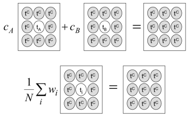
Figure 2: A pictorial illustration of the SS-CPA for a binary, A${}_{c_{A}}$B${}_{c_{B}}$, alloy (top) and of the GCPA (bottom). The rectangular frames have the meaning ”the Green function of what is inside”.

Eq. (27) is illustrated in Fig. (2). In terms of the ’coherent’ scattering-path matrix of the effective lattice, $\underline{\tau}^{c}$, and of the CPA ’projectors’, $\underline{D}_{i}$, it can be rearranged as follows:

$$\sum_{i}\frac{w_{i}}{N}\underline{D}_{i}=\underline{1}$$ (28)

$$\underline{D}_{i}=\left[\underline{1}+\left(\left(\underline{t}_{i}\right)^{-1}-\left(\underline{t}^{c}\right)^{-1}\right)\underline{\tau}^{c}\right]^{-1}$$ (29)

A GCPA theory is then an approximation for the $\underline{\underline{\tau}}$ matrix, whose diagonal elements are given by

$$\underline{\tau}_{ii}=\underline{D}_{i}\;\underline{\tau}^{c}$$ (30)

while the diagonal matrix elements of the Green function are given by Eq. (II.1) with $i=j$.

Within the approximation defined by Eqs. (27-30) above, the MST reviewed in the previous Section allows to calculate the charge densities and the integrated DOS, $N(\varepsilon,\mu)$ and, through Eq. (9), the kinetic part of the Hohenberg-Kohn functional. Here we need not to trace all the intermediate steps that can be reproduced following the scheme of Ref. Johnson et al. (1990). The GCPA approximate version of the Lloyd formula, Eq. (4), is given by:

$$\frac{N(\varepsilon;\mu)}{N} = \frac{N^{0}(\varepsilon)}{N}+\frac{1}{\pi}Im\sum_{i}w_{i}Tr\ln\underline{\tau}^{c}(\varepsilon)$$ (31)

$$+ \frac{1}{\pi}Im\sum_{i}w_{i}Tr\ln\underline{D}_{i}(\varepsilon)$$

It has the very remarkable property that the integrated DOS $N(\varepsilon;\mu)$ and, hence, the kinetic functional are variational Johnson et al. (1990) wrt. both $\underline{t}^{c}$ and $\underline{\tau}^{c}$.

In Sec. II A, we have mentioned that in the exact MST the contributions to the integrated DOS associated with each lattice site and proportional to $(ln\underline{\tau})_{ii}$, are coupled together because each element of the $\underline{\underline{\tau}}$ matrix depends on the scattering properties of all the lattice sites. Within the GCPA, the only source of coupling is $\underline{\tau}^{c}$. Each local contribution depends on $\underline{\tau}^{c}$ and on the local potential. However, within the GCPA, the Lloyd formula does not depend on $\underline{\tau}^{c}$ nor on the local potentials. As a consequence, the integrated DOS results in a sum of local contributions, coupled together only through $\underline{\tau}^{c}$,

$$N(\varepsilon;\mu)=\sum_{i}w_{i}N_{i}(\varepsilon;\mu)$$ (32)

We shall call this very controlled and tractable kind of coupling marginal coupling.

In view of further developments, it is convenient to isolate in Eq. (32) two distinct terms. The first arises from the first two addends in Eq. (31), it is identical for all sites and related to the effective background defined by the GCPA medium. The second depends on the local CPA projectors and, through them, on the local potentials. In formulae:

$$N_{i}(\varepsilon;\mu)=N_{i}^{back}(\varepsilon;\mu)+\frac{1}{\pi}ImTr\log\underline{D}_{i}(\varepsilon)$$ (33)

Implementing the GCPA within the DFT gives for the kinetic functional of Eq. (9) the following marginally coupled form:

$$T-\mu N=T^{back}(\mu)+\sum_{i}w_{i}T_{i}([\rho_{i}],\mu)$$ (34)

where

$$T^{back}(\mu)=-\int_{-\infty}^{\mu}d\varepsilon N^{back}(\varepsilon;\mu)$$ (35)

and

$$T_{i}([\rho_{i}],\mu) = \frac{1}{\pi}ImTr\int_{-\infty}^{\mu}d\varepsilon\log\underline{D}_{i}(\varepsilon)$$ (36)

$$- \int_{v_{i}}d\mathbf{r}\rho_{i}(\mathbf{r};\mu)v_{i}^{eff}(\mathbf{r};\mu)$$

As mentioned in Sect. II, in MST-based DFT calculations, the only source for $O(N^{3})$ scaling is the inversion of the multiple scattering matrix, Eq. (4), required to obtain the scattering-path matrix $\underline{\underline{\tau}}$. This step is bypassed in a GCPA theory by approximating the relevant matrix elements $\underline{\tau}_{ii}$ via Eq. (28) in terms of the local scattering properties and the coherent scattering matrix $\underline{\tau}^{c}$, the last of which is, in turn, obtained by an averaging process. For this reason, GCPA theories are $O(N)$, allowing for very substantial savings of computing time. Of course, the price for these savings is payed by the approximation implied by Eq. (30). A diagrammatic analysis of these errors can be found in Ref. Gonis, 1992.

It is necessary to make a couple of remarks about the physical meaning of the GCPA in the present context and to highlight the differences with respect to the traditional way in which CPA-based theories have been introduced in the past. In first place, the GCPA has been introduced here as an approximation for the Hohenberg-Kohn density functional. As an approximation, it may well be used to describe an ordered alloy. Its range of applicability is by no means confined to the realm of random alloys. In second place, the introduction of the weights $w_{i}$ to be assigned to each scatterer makes GCPA theories suitable for dealing with sophisticated pictures of the order (or the disorder) in metallic alloys. This, of course, requires what we have called an ’external model’. In a foregoing paper we shall discuss a (to some extent) self-consistent way to define an external model that is able to provide a picture of ordering phenomena in metallic alloys as a function of the temperature.

III.2 The DFT-MST-GCPA functional: the ’marginal coupling’ property

In the present subsection we shall analyze certain formal properties of the GCPA approximations introduced in the previous subsection. All the above discussion can be summarized in the following approximate density functional:

$$\Omega^{GCPA} = T^{back}(\mu)+\sum_{i}w_{i}\bigg{[}\omega^{GCPA}_{i}([\rho_{i}],\mu)$$ (37)

$$+ \frac{e^{2}}{2}\sum_{L}q_{i,L}V^{MAD}_{i,L}\bigg{]}$$

In Eq. (37) the $q_{i,L}$ are defined by Eq. (17) and the local part of the GCPA functional by

$$\omega^{GCPA}_{i}([\rho_{i}],\mu)=T_{i}([\rho_{i}],\mu)+u_{i}([\rho_{i}],\mu)$$ (38)

where the terms $T_{i}([\rho_{i}],\mu)$ and $u_{i}([\rho_{i}],\mu)$ are given by Eqs. (36) and (22) above. We note that the local GCPA functional, $\omega^{GCPA}_{i}$, depends also on the atomic number of the atom at $\mathbf{R}_{i}$, $Z_{i}$, and on the volume and the shape of the $i-th$ Voronoi polyhedron through the local potential energy term, $u_{i}$. In the following we shall make the simplifying assumpion of having identical Voronoi polyhedra for all the sites considered.

In Eq. (37) the coupling potentials, $V^{MAD}_{i,L}$, are provided by the specific external model. In the following of this Section we shall assume:

$$V^{MAD}_{i,L}=\sum_{j\neq i}\sum_{L^{\prime}}\lambda_{L}\lambda_{L^{\prime}}w_{j}M_{ij,LL^{\prime},}q_{j,L^{\prime}}$$ (39)

Appropriate choices of the coefficients $\lambda_{L}$ and of the weights, $w_{i}$, give then the SS-CPA or the PCPA. Furthermore, Eq. (39) can also be used for spherical or for full-potential charge reconstructions.

As mentioned in Sect. II A, Eq. (12), the density functional is variational not only wrt the global charge density, $\rho(\mathbf{r})$, and the chemical potential $\mu$, but also wrt the charge densities in each scattering volume, $\rho_{i}(\mathbf{r})$. Moreover, as discussed in Sec. III A and in Ref. Johnson et al., 1990, the GCPA density functional is variational wrt the effective medium scattering matrix, $\underline{\tau}^{c}$. Furthermore, in a GCPA theory, the background kinetic term, $T^{back}(\mu)$ in Eq. (37) depends on the electronic density only through $\underline{\tau}^{c}$ and $\mu$. Thus, the functional derivation of Eq. (37) wrt the local densities, $\rho_{i}(\mathbf{r})$, gives the following set of coupled equations:

$$\frac{\delta\omega^{GCPA}_{i}}{\delta\rho_{i}(\mathbf{r})}+V^{MAD}_{i}(\mathbf{r})=0$$ (40)

where we have used Eqs. (17), (18), (19) and (21).

Within a GCPA theory, solving the set of the Euler-Lagrange equations (40), one for each scattering center, together with the equations that determine the chemical potential and the coherent scattering matrix $\underline{\tau}^{c}$, is completely equivalent to the minimization of the density functional. As it is apparent, these Euler-Lagrange equations are coupled each other only through the Madelung potentials, $\underline{\tau}^{c}$ and $\mu$. Moreover, the functionals $\omega^{GCPA}_{i}(\rho_{i}(\mathbf{r}))$ are identical for sites occupied by the same chemical species.

In order to understand the consequences of the above result let us consider, for instance, an alloy sample constituted by a large supercell. One may wish to calculate, in the given sample, the properties of different ’atoms’, in first place the charge densities, $\rho_{i}(\mathbf{r})$. Inside the sample, $\underline{\tau}^{c}$, $\mu$ and the cell geometry are fixed, thus the set of the $\rho_{i}(\mathbf{r})$ is completely determined by the values of the Madelung potentials $V^{MAD}_{i}(\mathbf{r})$ and by the atomic number $Z_{i}$ of the ion at the position ${\mathbf{R}_{i}}$. More generally, inside the given sample, any site diagonal property $\Pi_{i}$ shall be completely determined by $Z_{i}$ and by the set of Madelung potentials. We can establish this result as follows:

$$\Pi_{i}=\Pi(Z_{i},V_{i}^{MAD}(\mathbf{r}))$$ (41)

Examples of such site diagonal properties are the local contributions to the grand potential, the multipole moments, and the local DOS. The functional forms, one for each alloying species, given by Eqs. (41) sometimes can be easily numerically fitted and then constitute a useful tool for the evaluation of the site quantities in the given sample. They are the source of the simple laws, as e.g. the ’qV’ laws, empirically found from extended metallic systems calculations. This notwithstanding, GCPA theories are able to predict complex trends for certain site diagonal properties as, e.g., the site resolved DOS’s Pella et al. (2004); Mammano et al. (2007).

Since Eqs. (41) allows to evaluate, among other properties, also the charge density of each fragment and, hence, the full charge density, $\rho(\mathbf{r})$, then, in virtue of the Hohenberg and Kohn theorem, it follows that any ground state observable in the sample given is a functional of the set of the Madelung potentials at all the crystal sites, $V^{MAD}_{i}(\mathbf{r})$, and of the set of the atomic numbers only. Since the last is, again, specified by the sample, it follows the theorem: any ground state observable in the sample given is a functional of the Madelung potentials only, or, equivalently, a function of the set of coefficients, $\{V^{MAD}\}$, that completely determine the Madelung potentials.

Since, in virtue of Eq. (39), the coefficients in the set $\{V^{MAD}\}$ are linear functions of the set of the multipole moments, $\{q\}$, then the above theorem implies the corollary that any ground state property of the sample is a function of the same moments. Within the GCPA and for the specific sample given, it is then possible to reformulate the DFT in terms of the charge multipole moments. By neglecting a constant term with the physical meaning of the grand potential contribution due to the mean GCPA ’atom’, Eq. (37) can be written as

$$\widetilde{\Omega}^{GCPA}(\{q\},\mu)=\sum_{i}w_{i}\widetilde{\omega}^{GCPA}_{i}(\{q_{i}\},Z_{i})$$

$$+\frac{e^{2}}{2}\sum_{i,j,L,L^{\prime}}w_{i}w_{j}\lambda_{L}\lambda_{L^{\prime}}M_{ij,LL^{\prime}}q_{i,L}q_{j,L^{\prime}}$$

$$-\mu\sum_{i}w_{i}q_{i,00}$$ (42)

In deriving Eq. (III.2), we have used Eq. (39) and the fact that, since $\omega^{GCPA}_{i}$ is completely determined by the local density, $\rho_{i}(\mathbf{r})$, it cannot depend on the multipole moments at other sites. Moreover, we have isolated the contribution proportional to the chemical potential, $\mu$. Having introduced an explicit dependence on $\mu$, the last term in Eq. (III.2) can be thought as a way of enforcing the global electroneutrality. This is unnecessary if we consider a specified sample in which, of course, $\mu$ has a precise, fixed vale. However, since the term proportional to $\mu$ has precisely the form it must have, its introduction is equivalent to extend the validity of Eq. (III.2) to all samples specified by the same mean atomic concentrations and by the same value for $\underline{\tau}^{c}$.

To summarize, we have established the following results. Within the GCPA class of approximations the Hohenberg and Kohn density functional can be recast in the form of Eq. (III.2). It consists of (a) local terms, $\widetilde{\omega}^{GCPA}_{i}$ for the $i$-th scattering site, consisting in functions of the charge multipole moments that are identical for sites with the same chemical occupation; (b) a bilinear form coupling the charge multipole moments at different sites, with coupling coefficients $M_{ij,LL^{\prime}}$ defined by the crystal geometry; (c) a term proportional to the chemical potential that ensures the global electroneutrality. The functional defined by Eq. (III.2) is identical for all the alloy samples characterized by the same mean atomic concentrations and the same value for the coherent scattering-path matrix $\underline{\tau}^{c}$. Evidently, it constitutes a coarse grained version of the DTF because the mathematical definition of the multipole moments, Eq. (17), does not completely determine the charge density. The last is determined by the multipole moments only within the GCPA theory. This reduction of the relevant information has been obtained at the price (a) of the GCPA approximation and (b) of having restricted the consideration to a specific sample. Nevertheless, no restriction has been made about the size of the sample that, therefore can be chosen in such a way to guarantee an appropriate description for a fixed concentration ensemble, as we shall discuss at the end of the present section.

Having recast the GCPA functional as a sum of functions of the charge multipole moments has obvious mathematical advantages. However, we have not yet completely determined the functional form of the local energetic contributions $\widetilde{\omega}^{GCPA}_{i}(\{q_{i}\},Z_{i})$. In order to do this, we need to make the hypothesys that, in the sample considered, the distribution of the Madelung potentials coefficients, $\{V^{MAD}\}$, is continuous in the range of the values that the same potentials assume in the sample. This is consistent with the observations in Refs. Faulkner et al., 1995, Faulkner et al., 1997, Bruno et al., 2003. Let us consider two scattering sites, say $i$ and $j$, occupied by the same chemical species, $\alpha$, at which the Madelung coefficients take very close numerical values, $V^{MAD}_{i,L}=V^{MAD}_{L}$ and $V^{MAD}_{j}(\mathbf{r})=V^{MAD}(\mathbf{r})+\Delta V^{MAD}(\mathbf{r})$. The local energetic contributions, the charge densities and the local multipole moments shall be: $\tilde{\omega}^{GCPA}_{i}=\tilde{\omega}^{GCPA}_{\alpha}$, $\rho_{i}(\mathbf{r})=\rho(\mathbf{r})$ and $q_{i,L}=q_{L}$ for the $i$-th site, and $\tilde{\omega}^{GCPA}_{j}=\tilde{\omega}^{GCPA}_{\alpha}+\Delta\tilde{\omega}^{GCPA}_{\alpha}$, $\rho_{j}(\mathbf{r})=\rho(\mathbf{r})+\Delta\rho(\mathbf{r})$ and $q_{j,L}=q_{L}+\Delta q_{L}$ for the $j$-th site. To the first order in $\Delta\rho(\mathbf{r})$ we have:

$$\Delta\tilde{\omega}^{GCPA}_{\alpha} = \int_{v_{i}=v_{j}}d\mathbf{r}\bigg{(}\frac{\delta\tilde{\omega}^{GCPA}_{\alpha}}{\delta\rho(\mathbf{r})}\bigg{)}_{\rho_{i}(\mathbf{r})=\rho(\mathbf{r})}\Delta\rho(\mathbf{r})$$

$$= -\int_{v_{i}=v_{j}}d\mathbf{r}V^{MAD}(\mathbf{r})\Delta\rho_{(}\mathbf{r})$$

where Eq. (40) has been used. The substitutions of the expansion for the Madelung potential, Eq.(18), and of the expressions for the charge multipole moments, Eq.(17), then give:

$$\Delta\tilde{\omega}^{GCPA}_{\alpha}=-\sum_{L}V^{MAD}_{L}\Delta q_{L}$$ (43)

Once integrated over $q_{L}$ Eq. (43) gives

$$\tilde{\omega}^{GCPA}_{\alpha}(\{q\})=\tilde{\omega}^{GCPA}_{\alpha}(\{q^{0}\})-\sum_{L}\int_{\{q^{0}\}}^{\{q\}}V^{MAD}_{L,\alpha}(\{q\prime\})dq_{L}^{\prime}$$ (44)

Eq. (44) can be easily numerically evaluated from the ’qV’ data, $V^{MAD}_{L,\alpha}=V^{MAD}_{L,\alpha}(\{q\})$ obtained as an output from GCPA calculations. Unless a constant with the meaning of the local energy contribution at $\{q\}=\{q^{0}\}$, it determines the local energies for each chemical species $\alpha$. Eqs. (43) and (44) have been obtained under very broad conditions: the differentiability of the kinetic functional Lieb (1983); Englisch and Englisch (1984) and the monotonicity of the ’qV’ laws. The first is the usual requirement for the convergence of the Kohn-Sham scheme of the DFT, while the second condition is certainly verified by all GCPA calculations reported in the literature, including those executed at extremely high values for the Madelung potential (see Fig. 7 in the next subsection and the related discussion).

In the remainder of the present Section we shall make a few general comments about the validity of the framework defined by the GCPA theory in comparison with the exact density functional.

(i) The fact that the effective potential and the potential energy functional can be decomposed in site contributions coupled together only through the Madelung potentials is an exact consequence of the LDA and it has nothing to do with the GCPA. This kind of coupling is ’marginal’ in the sense that, although not necessarily small, it has the simple and tractable functional form which arises from the bilinear terms involving the multipole moments in Eq. (III.2). Although this is beyond the purpose of the present paper, we notice that most non-local density functionals offered in the literature Dreizler and Gross (1990); Dreizler and da Providencia (1985) are actually local wrt the density gradients, thus most non-local schemes will remain marginally coupled in the above sense.

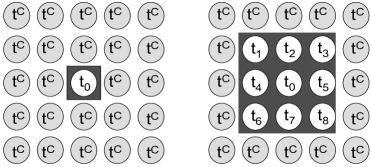
Figure 3: The Local Interaction Zones (LIZ) used in PCPA (left frame) and LSGF (right frame) calculations are marked by the dark areas. For each scattering site, the kinetic functional is evaluated using the appropriate single-site scattering matrices, $t_{i}$, inside the LIZ, and the effective CPA scattering matrix, $t^{c}$, outside.

(ii) Splitting the kinetic functional into local contributions marginally coupled trough the coherent scattering matrix $\underline{\tau}^{c}$ is a simplification due to the GCPA. In fact, it has been obtained by assuming averaged boundary conditions at the surfaces of the Voronoi polyhedra through Eq. (27). An estimate of the so induced errors can be obtained by the comparison of PCPA vs. Locally Self-Consistent Green Function (LSGF) calculations Abrikosov et al. (1996) executed on the same supercell. As it is sketched in Fig. (3), both calculations evaluate the kinetic contribution from the $i$-th to the functional by solving the problem of a single impurity, in the case of the PCPA, or of an impurity cluster, the Local Interaction Zone (LIZ), for the LSGF. In both cases the scattering matrices outside the LIZ are set to the coherent scattering matrix, $\underline{t}^{c}$. PCPA calculations can then be viewed as LSGF calculations with only one atom in the LIZ. This argument also suggest that, wrt GCPA calculations, exact DFT results include, for each site, corrections depending on its chemical environment.

(iii) We have already seen that the coarse grained version of the GCPA functional, Eq. (III.2), holds for all the alloy configurations characterized by a specified value for $\underline{\tau}^{c}$ in a fixed concentration ensemble. This could appear as a serious limitation since it looks unlikely that, e.g., $\underline{\tau}^{c}$ could have the same functional energy dependence for two different systems. In general, in a GCPA theory, $\underline{\tau}^{c}$ is a ground state property determined not only by the mean concentrations but also by the distributions of the Madelung potentials for each alloying species. As opposite to the SS model where these distributions are trivial, more sophisticated external models, as e.g. the PCPA, give complicated charge and Madelung potential distributions. How could then the GCPA functional be useful in such cases?

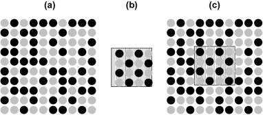
Figure 4: The PCPA supercells shown in frame (a) and (b) contains, respectively, $N\rightarrow\infty$ atoms in a random alloy configuration and $n$ atoms in an ordered configuration, both at the same mean atomic concentrations. $N$ is large enough to to guarantee an appropriate description of a random alloy within a GCPA theory. Similarly, $n$ has been chosen to permit the description of an ordered alloy up to some length scale $l$. The supercell in the frame (c) is identical to that in (a) except but for the dashed region which contains $n$ atoms in the same ordered configuration as in (b). The cell (c) is therefore able to describe an ordering fluctuation up to the scale set by $l$.

As argued by Faulkner et al. Faulkner et al. (2001b), the PCPA theory applied to ideal random alloys gives well-defined values for all physical properties. This is because, in perfect random alloys, the distribution of the chemical environments is easily obtained by statistical considerations and it is given by the appropriate multinomial distributions. Therefore, the PCPA random alloy constitutes a privileged reference system whose physical properties, including $\underline{\tau}^{c}$, can be approximated up to an arbitrary accuracy by letting the number of atoms in the PCPA supercell, $N$, going to infinity (see Fig. 4a). We believe that the same $\underline{\tau}^{c}$ obtained for a random alloy at a given concentration can be used for building a physically clean, though approximate, theory also for ordered alloys at the same concentration. In the next section we shall provide numerical evidences for that, here we present a more formal argument. Imagine that an ordered array containing $n$ atoms (Fig.4b) is able to account for the properties of same ordered alloy configuration, up to a length scale, $l$, that can be made large at will in the $n\rightarrow\infty$ limit. In Fig. 4c we draw a supercell, a part of which is constituted by the supercell of Fig. 4b, while the remaining $N-n$ sites are occupied as in the random alloy supercell of Fig. 4a. We can think that the supercell in Fig. 4c represents a fluctuation of an ordered phase in a random alloy matrix and that it describes the physical properties of such fluctuation up to the same length scale $l$ as in Fig. 4b. We are implicitly using the common idea of ’locality’ in physics, or, in a more specific context, of ’nearsightedness’ of the DFTKohn (1996). However, as Eq. (28) implies, the difference between the coherent scattering-path matrices corresponding to Figs. 4a and 4c, $\underline{\tau}^{c}_{a}-\underline{\tau}^{c}_{c}$, is proportional to the ratio $n/N$ and, then, it can be made small at will in the $N\rightarrow\infty$ limit, for any value of $n$. We conclude that the coherent scattering-path matrices of a random alloy, $\underline{\tau}^{c}_{a}$, is able to account for the physical properties of ordered configuration considered. The limitation $n/N<<1$, that comes from the above argument, does not impose any upper bound on the maximum length scale at which chemical fluctuations can be studied and it is of no practical importance provided that $N$ is large enough to ensure a good approximation $\underline{\tau}^{c}_{a}$. As reported in the literature Pella et al. (2004); Faulkner et al. (2006), it seems that $N$ about 100 is already enough.

iv) Although we have suggested that the coherent scattering matrix from random alloys GCPA calculations can be used for ordered alloys too, we are aware of the limitations of such a physical picture. For instance, a GCPA theory always implies finite quasiparticle lifetimes Bruno et al. (1994), and, hence, a smearing of the peaks of the Bloch spectral function (BSF).

III.3 A generalized version of the Charge Excess Functional Theory

As a matter of fact, the analysis of DFT supercell calculations for metallic alloys suggests the existence of simple relationships between the charge excesses at the lattice sites, $q_{i,00}$, and the Madelung potentials at the same sites, $V^{MAD}_{i,00}$. Namely, simple linear laws, one for each alloying species, have been found to hold, say

$$a_{i}q_{i,00}+V^{MAD}_{i,00}=k_{i}$$ (45)

where $a_{i}$ and $k_{i}$ have the same numerical values for atoms of the same chemical species in the given supercell. Examples of the linear ’qV’ laws obtained from PCPA calculations for a binary and a quaternary alloy are reported in Figs. 5 and 6.

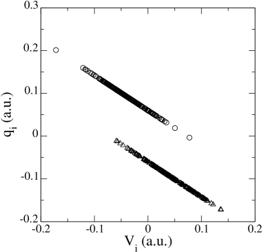
Figure 5: ’qV’ relationships for a bcc random $Cu_{0.50}Zn_{0.50}$ alloy. The excesses of electrons, $q_{i}=q_{i,00}$ are plotted vs. the Madelung potentials, $V^{MAD}_{i}$. The results have been obtained from $\ell_{MAX}=0$ PCPA calculations for a supercell containing 432 atoms at lattice costant $a=5.50$ a.u.. Circles represent Cu atoms and triangles Zn atoms. Note that positive values for $q_{i}$ correspond to negative net charges and vice versa.

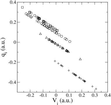
Figure 6: ’qV’ relationships for an fcc random $Al_{0.25}Cu_{0.25}Ni_{0.25}Zn_{0.25}$ alloy. The excesses of electrons, $q_{i}=q_{i,00}$ are plotted vs. the Madelung potentials, $V^{MAD}_{i}$. The results have been obtained from $\ell_{MAX}=0$ PCPA calculations for a bcc supercell containing 108 atoms at lattice costant $a=6.88$ a.u.. Circles, squares, triangles and crosses stand for Cu, Ni, Zn and Al atoms.

It is interesting to observe that similar linear ’qV’ laws can be derived starting from the GCPA functional, Eq. (III.2), for random alloys by a second order series expansion about the zero Madelung field multipole moments, $\{q^{0}\}$, that can be obtained by solving the following set of equations:

$$\frac{\partial\widetilde{\omega}^{GCPA}_{i}}{\partial q_{i,L}}=0$$ (46)

This procedure leads to a Ginzburg-Landau configurational ’Hamiltonian’ in which the relevant fields are constituted by the values of the multipole moments of each lattice site. In formulae:

$$\widetilde{\Omega}^{CEF}(\{q\},\mu)=\frac{1}{2}\sum_{i,L,L^{\prime}}w_{i}a_{i,LL^{\prime}}(q_{i,L}-q^{0}_{i,L})(q_{i,L^{\prime}}-q^{0}_{i,L^{\prime}})+\frac{1}{2}\sum_{i,j,L,L^{\prime}}w_{i}w_{j}\lambda_{L}\lambda_{L^{\prime}}M_{ij,LL^{\prime}}q_{i,L}q_{j,L^{\prime}}-\mu\sum_{i}q_{i,00}$$ (47)

where we have omitted the term $\widetilde{\Omega}^{CEF}(\{q^{0}\},\mu=0)$ that represent the GCPA energy at zero Madelung field and chemical potential and that is constant in a fixed concentration ensemble. The coefficients $a_{i,LL^{\prime}}$ are given by the second derivatives of the GCPA functional

$$a_{i,LL^{\prime}}=\bigg{(}\frac{\partial^{2}\widetilde{\omega}^{GCPA}_{i}(\{q_{i}\})}{\partial q_{i,L}\partial q_{i,L^{\prime}}}\bigg{)}_{\{q_{i}\}=\{q^{0}_{i}\}}$$ (48)

The functional of Eq. (47) constitutes a generalization of the Charge Excess Function (CEF) proposed in Ref. Bruno et al., 2003 for discussing the charge transfers in metallic alloys and shall then be referred in the following to as the CEF. The novel feature here is that Eq. (47) includes not only the charge excesses, $q_{i,00}$, but also the charge multipole moments with $\ell>0$.

The minimization of the CEF functional $\widetilde{\Omega}^{CEF}$ wrt. its variables, the set of the multipole moments, $\{q\}$, and the chemical potential, $\mu$, gives

$$\sum_{L^{\prime}}\big{[}a_{i,LL^{\prime}}(q_{i,L^{\prime}}-q^{0}_{i,L^{\prime}})+M_{LL^{\prime},ij}\;q_{j,L^{\prime}}\big{]}=\mu\delta_{i,00}$$ (49)

and

$$\sum_{i}q_{i,00}=0$$ (50)

Using the definition of the Madelung potentials, Eq. (39), and setting

$$k_{i,L}=\sum_{L^{\prime}}a_{i,LL^{\prime}}q^{0}_{i,L^{\prime}}+\mu\delta_{i,00}$$ (51)

it is easy to show that Eq. (49) for $L=(0,0)$ coincides with the linear laws given by Eq. (45). Versions of Eqs. (49), (50) and (51) with the angular momentum summations truncated at $\ell=0$ can be found in Ref. Bruno et al., 2003.

We wish to highlight that the CEF derivation from the GCPA functional is based on the assumption, common to all Ginzburg-Landau theories Khachaturyan (1983); S2 , that the homogeneously disordered phase, in the present case the random alloy phase, can the starting point for a perturbative treatment of ordering or segregation phenomena. As discussed in the previous subsection, in the GCPA context, this amounts to conjecture that the coherent scattering-path matrix $\underline{\tau}^{c}$ of a random alloy can be used for obtaining a physical picture of concentration fluctuations, or, in other words, that it is able to represent such fluctuations.

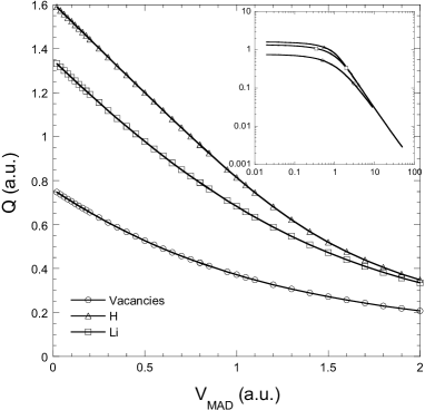
Figure 7: ’qV’ relationships for light substitutional impurities (vacancies, H and Li atoms) dissolved in bcc Al, from CPA+LF calculations. The quantity $Q$ is the number of valence electrons at the impurity site, therefore $Q=0$ corresponds to 0 electrons for vacancies and H atoms and 2 electrons for Li. The linear behaviors observed for small fields ($V_{MAD}<\;1\;a.u.$) are superseded by power law trends (see the log-log plot in the inset) for very high fields.

We wish to close this Section with a few comments. The principal result of this paragraph, the CEF functional of Eq. (47), has been obtained by a series expansion of the GCPA functional about the values that the multipole moments would have in absence of coupling. The series has been terminated at the lowest order at which differences with respect to SS approximations are expected for. This, not surprisingly, is enough to obtain a physical picture of the charge transfers in metallic alloys. For a given alloy configuration, the linear Euler-Lagrange equations obtained by minimizing the CEF can be easily solved for the charge multipole moments. The procedure require the inversion of the matrix $\underline{\underline{F}}$ of elements

$$F_{ij,LL^{\prime}}=a_{i,LL^{\prime}}\;\delta_{ij}+M_{ij,LL^{\prime}}$$ (52)

As we have shown elsewere Bruno et al. (2003); Bruno (2007), for a given alloy configuration, the value of the CEF functional at its minimum has the physical meaning of the total energy of the same configuration. The ambiguity due to the presence of the above mentioned concentration dependent constant can be resolved by comparing CEF and GCPA calculations for a single configuration in a fixed concentration ensemble.

In the previous subsection we have described a general procedure based on the numerical integration of the ’qV’ laws for evaluating the functional form of $\tilde{\omega}_{i}^{GCPA}(\{q_{i}\})$. Of course, if the random alloy $\underline{\tau}^{c}$ was able to represent concentration fluctuations and the ’qV’ laws were linear, the GCPA and the CEF functionals would be coincident. We do not think that the ’qV’ laws can be truly linear. The argument is as follows. The local excesses of electrons, $q_{i,00}$, accordingly with the physical intuition and with the results plotted in Figs. 5 and 6, are non-increasing functions of the Madelung potential $V^{MAD}_{i,00}$. If the ’qV’ laws were really linear, $q_{i,00}$ would decrease indefinitively and eventually reach unphysical values, $q_{i,00}<Z_{i}$ corresponding to negative charge densities. Actually we expect that the linear laws cannot be any longer valid when all valence electrons are expelled from the site. This circumstance would correspond to some critical value for the charge excess, say $q_{i,00}^{crit}$. Before this critical value is reached, the ’qV’ laws should exhibit a crossover to an asymptotic behavior, say $q_{i,00}\rightarrow q_{i,00}^{crit}$ as $V^{MAD}_{i,00}\rightarrow\infty$. We have tested this conjecture by executing CPA+LF calculations Bruno et al. (2002) for a single impurities, vacancies, H or Li atoms, embedded in Al. The results are shown in Fig. 7, where we plot $Q=q_{i,00}-q_{i,00}^{crit}$ for the impurity site as a function of the relevant Madelung fields. In all the cases considered, a linear regime is clearly visible at low fields. A very high fields, a crossover to a power law dependence is observed, with the number of electrons tending to the critical value from above. The crossover field is comparable with the host band width. We recall that in CPA+LF calculations $\underline{\tau}^{c}$ is that of the host while the Madelung potential is just an adjustable papameter. While this is a sensible way for studying the response of the impurity to the perturbing field, this do not imply that all the range of the perturbations considered is physically meaningful. We do not think that such high fields, corresponding to the tunneling regime in the impurity site, could occur in real systems as this would require a too large defect of electrons at the impurity nearest neighbors. Hence, Fig. 7, while supporting the view that the linearity of the ’qV’ laws and the CEF are just approximations, does not support the possibility that, at least for metallic systems, appreciable deviations from linearity or failures of the CEF are likely to occur.

Another point we wish to address is concerned with the value of the chemical potential $\mu$ in Eq. (47). In a recent paper, Drchal et al. Drchal et al. (2006) argued that $\mu$ should be always zero since the Fourier transform of the Madelung coefficients with $L=L^{\prime}=(0,0)$ diverges as $k\rightarrow\infty$ implying that the sum of the charge excesses $\sum q_{i,00}$ must vanish, automatically satisfying the electroneutrality constraint. The observation of Drchal et al. is correct for infinite systems, while for finite supercells, even with periodic boundary condition, the same Fourier transform always remains finite. $k$, in fact can take only the values of the reciprocal space vectors that consitute the tiling of the supercell considered Rowlands et al. (2005). The set of the allowed values for $k$ includes $0$ only for infinitely large supercells. In most practical calculations, then, $\mu$ is necessary, although usually it takes small non-zero values.

IV Numerical results

In this Section we present a series of numerical tests designed to study the limits of validity of the GCPA and CEF theoretical frameworks. The central issues here shall be investigating the realm of validity of the linear ’qV’ laws, Eq. (45) or (49), and of the energetics implied by the CEF functional, Eq. (47). Furthermore, we shall try to answer two questions: (i) to what an extent the CEF is able to approximate GCPA calculations and (ii) how do the predictions from the CEF and the GCPA compare vs. ’exact’ DFT calculations for ordered systems. The GCPA theory chosen for these tests is the PCPA Ujfalussy et al. (2000), that, being based on a supercell approach, allows for easy comparison vs. ’exact’ DFT calculations.

Several kinds of calculations shall be presented in this Section. The ’exact’ DTF results used for comparison shall be LDA full-potential LAPW calculations produced using the WIEN2K ab initio package Blaha et al. (2001); Schwarz et al. (2002). They are referred below to as LAPW. In all the cases about 10⁴ k-points in the full Brillouin zone have been used, the spherical harmonics expansion of the potentials in the muffin-tin spheres has been truncated at $\ell=6$ and the parameter $R_{MT}\cdot K_{MAX}$ has been set to 7. The PCPA calculations have been performed by a conveniently modified version of our KKR-CPA code Bruno and Ginatempo (1997). All PCPA calculations are based on the ASA approximation for the site potentials, use several thousands k-points in the full Brillouin Zone and 31 energies over a complex integration contour. For both LAPW and PCPA calculations, the core electrons treatment is fully relativistic while a non-relativistic approximation is used for valence states. Finally, we present CEF calculations Bruno et al. (2003); Bruno and Zingales (2004) with the charge multipolar expansion truncated at $\ell=0$. The concentration dependent parameters required by the CEF have been obtained from the linear regressions of the ’qV’ data generated from supercells with random occupancies and the required mean atomic concentrations and are reported in Tables 1 and  2. Depending on which was the source of the parameters, the CEF calculations shall be referred to as CEF-PCPA or CEF-LAPW. Using the formalism of the previous Section, for both PCPA and CEF calculations we set $w_{i}=1$ for all lattice sites, $\lambda_{00}=1$ and $\lambda_{\ell m}=0$ for $\ell>0$.

Table 1: CEF parameters obtained by the linear regression of the ’qV’ data from PCPA calculations for random Cu_cZn_1-c alloys in bcc or fcc lattices. $C_{Cu}$ and $C_{Zn}$ are defined as the difference between 1 and the correlations obtained from the regressions for the Cu and Zn site charges. All the quantities are expressed in atomic units. CEF calculations using the coefficients presented in this Table are referred to as CEF-PCPA.

	c	$a_{Cu}$	$a_{Zn}$	$k_{Cu}-k_{Zn}$	$C_{Cu}$	$C_{Zn}$
	0.20	1.223	1.211	0.146	3 10-7	1 10-6
	0.25	1.225	1.214	0.147	4 10-7	1 10-6
	0.33	1.223	1.215	0.148	5 10-7	2 10-6
bcc	0.50	1.219	1.214	0.146	5 10-7	2 10-6
	0.67	1.215	1.214	0.144	3 10-7	2 10-6
	0.75	1.214	1.214	0.144	3 10-7	2 10-6
	0.80	1.213	1.214	0.144	3 10-7	9 10-7
	0.20	1.220	1.212	0.138	3 10-7	1 10-6
	0.25	1.221	1.214	0.140	3 10-7	9 10-7
	0.33	1.222	1.216	0.142	3 10-7	1 10-6
fcc	0.50	1.222	1.217	0.143	5 10-7	2 10-6
	0.67	1.223	1.222	0.145	5 10-7	1 10-6
	0.75	1.222	1.223	0.145	3 10-7	1 10-6
	0.80	1.222	1.222	0.145	3 10-7	2 10-6

Table 2: CEF parameters obtained by the linear regression of the ’qV’ data from LAPW calculations for random Cu_cZn_1-c alloys in bcc or fcc lattices. $C_{Cu}$ and $C_{Zn}$ are defined as the difference between 1 and the correlations obtained from the regressions for the Cu and Zn site charges. All the quantities are expressed in atomic units. CEF calculations using the coefficients presented in this Table are referred to as CEF-LAPW.

	c	$a_{Cu}$	$a_{Zn}$	$k_{Cu}-k_{Zn}$	$C_{Cu}$	$C_{Zn}$
	0.25	2.968	2.181	0.456	3 10-2	2 10-2
	0.33	2.704	2.327	0.445	4 10-3	8 10-3
bcc	0.50	2.811	2.307	0.413	9 10-3	5 10-2
	0.67	3.388	3.351	0.590	3 10-3	7 10-3
	0.75	2.586	2.652	0.432	3 10-2	1 10-2
	0.25	2.457	1.949	0.360	5 10-3	9 10-4
fcc	0.50	2.287	2.130	0.350	9 10-3	3 10-3
	0.75	2.646	2.317	0.399	4 10-3	2 10-4

IV.1 qV laws

In Sect. III we have presented the CEF functional as an approximation for the GCPA functional and have shown how this is equivalent to assume the linearity of the ’qV’ laws. In Figs. (5) and (6), we plot the ’qV’ curves from our PCPA calculations for the binary bcc Cu_0.50Zn_0.50 and the quaternary Al_0.25Cu_0.25Ni_0.25Zn_0.25 fcc random alloys. It is surprising to observe how much accurately the PCPA data can be fitted by straight lines. The correlations coefficients obtained from the linear regression of the same data differ from unit by about $10^{-6}$. Similar very high correlations are always obtained from the analysis of PCPA ’qV’ data, as it is evident by looking at Table 1. As it is shown in Table 2, also LAPW data present high correlations, although the corresponding linear fits are not perfect and their correlations deviate from unit by $10^{-2}$ or $10^{-3}$. This notwithstanding, as argued in Sect. III C, we believe that the linearity of the ’qV’ relationships within the PCPA is just an approximation. In order to check out how much accurate it is, we have studied one of the most difficult realistic cases, that of a high charge transfer ordered alloy, namely the CuZn system. This system has been studied with many different theoretical approaches Althoff et al. (1996); Crisan et al. (2000); Muller and Zunger (2001); Rowlands et al. (2006); Tarafder et al. (2006); Tulip et al. (2006). It is also relevant, for our present concerns, that the total energy differences between fcc and bcc geometrical alloy arrangements are relatively small. We have executed calculations for all the set of 62 bcc and fcc based structures reported in Refs. Curtarolo et al., 2005 and Curtarolo, 2003. These structures include several ordered crystals for each of the the following Cu atomic concentrations: 0.20, 0.25, 0.33, 0.50, 0.66, 0.75 and 0.80. In order to facilitate the comparison, the lattice constants have been kept fixed to the values 5.5 and 6.9 a.u., respectively for bcc and fcc based lattices. The results for bcc- and fcc-based alloys are reported in Tables 3 and 4, respectively.

Table 3: Charge excesses and total energies per atom for bcc-based Cu_cZn_1-c alloys. The first two columns on the left give, for each system, the mean Cu atomic concentration ($c$) and, when available, the supercell identifier in the database of Ref. Curtarolo (2003) (conf). ”R” followed by a number, e.g., R16, stands for a quasirandom supercell containing the corresponding number of atoms not included in the database. In the third column $n_{unl}$ indicates the mean number of unlike nearest neighbors of Zn sites. The columns from 4th to 7th report the MSD of the charge excesses, $<(\Delta q)^{2}>$, obtained by the comparison of different theories: PCPA vs. CEF-PCPA (a), LAPW vs. CEF-PCPA (b), LAPW vs. CEF-LAPW (c), LAPW vs. the model of Ref. Magri et al., 1990 (d). Columns from 8th to 11th: total energies per atom from PCPA, CEF-PCPA, LAPW and CEF-LAPW calculations. The energy zero is given, for each concentration, by the PCPA prediction for the ground state.

			$<(\Delta q)^{2}>$				$\Delta E$ (mRy)
c	conf	$n^{unl}$	a	b	c	d	PCPA	CEF-PCPA	LAPW	CEF-LAPW
	92	1.5	5 10-11	1 10-4	-	-	0.038	0.040	-0.015	-
0.20	98	2.0	2 10-9	4 10-4	-	-	0.000	0.000	0.000	-
	69	2.0	3 10-9	4 10-5	2 10-6	-	0.741	0.742	0.991	0.556
	72	1.3	9 10-9	4 10-4	2 10-5	-	1.966	1.971	3.951	2.437
	75	2.0	1 10-9	1 10-5	1 10-6	-	0.824	0.823	1.089	0.631
0.25	78	2.7	1 10-9	4 10-4	5 10-7	-	0.865	0.864	0.980	0.838
	81	2.7	3 10-8	2 10-4	4 10-7	-	0.353	0.353	0.050	0.246
	83	2.7	2 10-8	3 10-4	1 10-6	-	0.327	0.327	0.194	0.260
	86	2.7	6 10-8	4 10-4	2 10-5	-	0.000	0.000	0.000	0.000
	R16	2.2	1 10-8	1 10-4	3 10-6	-	0.797	0.799	1.117	0.669
	63	3.0	3 10-8	2 10-4	2 10-5	-	0.000	0.000	0.000	0.000
0.33	65	2.0	2 10-9	3 10-4	2 10-5	-	1.741	1.747	2.950	2.129
	67	4.0	2 10-8	2 10-4	3 10-5	-	0.078	0.078	-0.519	0.068
	R18	3.3	6 10-9	3 10-4	4 10-5	-	0.558	0.562	0.729	0.838
	60	4.0	4 10-9	4 10-5	5 10-6	3 10-4	1.661	1.662	3.457	1.188
	61	8.0	3 10-9	1 10-3	6 10-6	3 10-3	0.000	0.000	0.000	0.000
	71	2.0	2 10-9	1 10-3	4 10-5	9 10-4	4.107	4.115	8.657	5.089
0.50	74	4.0	3 10-9	5 10-7	4 10-7	3 10-4	1.823	1.824	3.666	1.342
	77	4.0	4 10-11	2 10-4	1 10-6	7 10-5	2.736	2.739	4.804	2.404
	80	6.0	7 10-9	4 10-4	8 10-7	3 10-4	0.885	0.883	1.666	0.557
	85	4.0	7 10-9	2 10-4	1 10-5	7 10-4	1.007	1.006	2.757	0.646
	R16	4.3	3 10-9	2 10-4	3 10-6	4 10-4	1.989	1.989	3.806	1.613
	62	6.0	7 10-10	2 10-4	6 10-7	-	0.000	0.000	0.000	0.000
0.67	64	4.0	8 10-12	3 10-4	2 10-5	-	1.698	1.703	2.671	2.021
	66	8.0	2 10-10	1 10-4	2 10-7	-	0.076	0.077	-0.650	0.061
	R18	6.7	3 10-9	3 10-4	1 10-6	-	0.545	0.549	0.508	0.870
	68	6.0	2 10-11	2 10-5	1 10-6	-	0.726	0.732	1.364	0.566
	70	4.0	3 10-9	6 10-4	3 10-5	-	1.927	1.935	3.395	2.505
	73	6.0	2 10-10	9 10-6	2 10-6	-	0.806	0.812	1.390	0.642
0.75	76	8.0	1 10-9	5 10-4	4 10-6	-	0.850	0.852	1.022	0.873
	79	8.0	3 10-9	2 10-4	1 10-6	-	0.345	0.349	0.464	0.251
	82	8.0	4 10-9	3 10-4	2 10-6	-	0.322	0.323	0.462	0.269
	84	8.0	3 10-8	4 10-4	4 10-6	-	0.000	0.000	0.000	0.000
	R16	6.8	1 10-9	2 10-4	3 10-6	-	0.782	0.788	1.278	0.685
	87	6.0	5 10-10	1 10-4	-	-	0.033	0.038	0.327	-
0.80	93	8.0	4 10-10	6 10-4	-	-	0.000	0.000	0.000	-

The charges from the CEF-PCPA are, in practice, identical to those obtained from the PCPA theory for the ordered systems. In order to represent the size of these tiny differences, we report in Tables 3 and 4 the mean square displacement between the two sets of calculated charges, $<(\Delta q)^{2}>$. In the worst case, the bcc-based DO₂ structure, identified in Table 4 by the number 86, we find $<(\Delta q)^{2}>=6~{}10^{-8}$. Such an excellent agreement has been obtained for all the set of ordered structures considered, in spite of the fact that the CEF input has been obtained from random supercells.

Table 4: Charge excesses and total energies per atom for fcc-based Cu_cZn_1-c alloys. The first two columns on the left give, for each system, the mean Cu atomic concentration ($c$) and, when available, the supercell identifier in the database of Ref. Curtarolo (2003) (conf). ”R” followed by a number, e.g., R16, stands for a quasirandom supercell containing the corresponding number of atoms not included in the database. In the third column $n_{unl}$ indicates the mean number of unlike nearest neighbors of Zn sites. The columns from 4th to 7th report the MSD of the charge excesses, $<(\Delta q)^{2}>$, obtained by the comparison of different theories: PCPA vs. CEF-PCPA (a), LAPW vs. CEF-PCPA (b), LAPW vs. CEF-LAPW (c), LAPW vs. the model of Ref. Magri et al., 1990 (d). Columns from 8th to 11th: total energies per atom from PCPA, CEF-PCPA, LAPW and CEF-LAPW calculations. The energy zero is given, for each concentration, by the PCPA prediction for the ground state.

			$<(\Delta q)^{2}>$				$\Delta E$ (mRy)
c	conf	$n^{unl}$	a	b	c	d	PCPA	CEF-PCPA	LAPW	CEF-LAPW
	35	2.5	3 10-10	2 10-5	-	-	0.500	0.503	0.926	-
0.20	39	3.0	7 10-9	7 10-5	-	-	0.000	0.000	0.000	-
	12	3.3	2 10-9	7 10-5	4 10-6	-	0.515	0.516	1.078	0.438
	15	2.7	1 10-8	2 10-4	4 10-7	-	1.379	1.386	2.151	1.658
	18	3.3	2 10-9	2 10-5	2 10-6	-	0.566	0.568	1.054	0.471
0.25	21	3.3	2 10-9	1 10-4	8 10-6	-	0.680	0.685	1.510	0.616
	24	4.0	2 10-8	2 10-4	5 10-6	-	0.000	0.000	0.000	0.000
	26	4.0	2 10-8	2 10-4	3 10-7	-	0.068	0.069	0.073	0.051
	29	2.0	5 10-9	4 10-4	2 10-5	-	1.817	1.824	4.202	2.349
	R16	3.0	1 10-8	2 10-4	1 10-6	-	1.015	1.020	1.705	1.169
	6	4.0	1 10-10	5 10-5	-	-	1.179	1.185	1.016	-
0.33	8	5.0	1 10-8	1 10-4	-	-	0.000	0.000	0.000	-
	10	3.0	6 10-11	3 10-4	-	-	1.800	1.807	3.300	-
	3	8.0	7 10-9	3 10-4	5 10-6	1 10-4	0.139	0.144	-0.075	0.111
	4	6.0	2 10-9	5 10-6	2 10-5	6 10-5	1.075	1.081	2.141	0.961
	14	4.0	1 10-9	6 10-4	5 10-6	2 10-4	2.895	2.905	4.803	3.657
0.50	17	7.0	3 10-9	3 10-5	2 10-6	1 10-6	0.717	0.720	1.121	0.605
	20	6.0	5 10-10	5 10-5	1 10-7	5 10-5	1.429	1.434	2.464	1.353
	23	8.0	7 10-9	2 10-4	1 10-6	4 10-5	0.000	0.000	0.000	0.000
	28	3.0	2 10-9	9 10-4	6 10-5	5 10-4	3.339	3.350	6.745	4.694
	R16	6.8	3 10-9	2 10-4	2 10-6	6 10-5	0.913	0.918	1.519	0.972
	5	8.0	3 10-10	9 10-5	-	-	1.102	1.224	1.283	-
0.67	7	10.0	1 10-8	1 10-4	-	-	0.000	0.000	0.000	-
	9	6.0	3 10-9	3 10-4	-	-	1.743	1.866	3.224	-
	11	10.0	3 10-10	9 10-5	2 10-5	-	0.549	0.550	1.009	0.501
	13	8.0	5 10-9	5 10-4	3 10-6	-	1.479	1.482	2.230	1.986
	16	10.0	3 10-10	2 10-5	1 10-5	-	0.604	0.605	1.054	0.535
0.75	19	10.0	5 10-10	1 10-4	5 10-6	-	0.729	0.731	1.083	0.709
	22	12.0	3 10-9	2 10-4	5 10-6	-	0.000	0.000	0.000	0.000
	25	12.0	2 10-9	2 10-4	5 10-6	-	0.073	0.073	-0.193	0.057
	27	6.0	1 10-8	5 10-4	1 10-5	-	1.944	1.949	3.654	2.799
	R16	3.0	2 10-9	3 10-4	2 10-6	-	1.088	1.091	1.790	1.409
	30	10.0	1 10-9	6 10-5	-	-	0.544	0.550	-4.023	-
0.80	36	12.0	2 10-8	7 10-5	-	-	0.000	0.000	0.000	-

In a previous Letter Bruno et al. (2003) we have shown that the CEF is able to carefully reproduce the charges from LSMS calculations. Moreover, the parameters extracted from ordered structure calculations can be used to predict the charges for random structures and vice-versa. The quality of the CEF predictions was very good either, with $<(\Delta q)^{2}>$ of the order of $10^{-6}$, i.e. about three orders of magnitude less than what we have found by the comparison of CEF and PCPA. Since the LSMS calculations presented in Ref. Bruno et al., 2003 were based on the ASA, we surmise that the modest lost of accuracy of CEF predictions for LSMS wrt. PCPA calculations constitutes a measure of the importance of the scattering effects from nearest neighbors. These effects, in fact, can be accounted for only in a mean field fashion by the PCPA.

We have also investigated the effects of the spherical approximation for the atomic potentials by executing full-potential LAPW calculations. In Fig. 8 we plot the site charge excesses obtained from LAPW vs. the number of unlike nearest neighbors of the same sites, for all the structures corresponding to equimolar concentrations. In Tables 3 and 4 we report the results for $<(\Delta q)^{2}>$ at all the concentrations. As apparent from Fig. 8, the trends of $q_{i}$ are not easily accounted for by the nearest neighbors environment only Magri et al. (1990), expecially for bcc based structures.

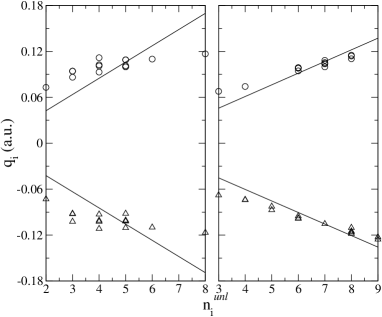
Figure 8: Charge excesses, $q_{i}$, vs. the number of unlike nearest neighbors of the corresponding site, $n^{unl}_{i}$, from LAPW calculations for many, bcc and fcc based, ordered and disordered, configurations, of $Cu_{0.50}Zn_{0.50}$ alloys. Circles and triangles represent charges on Cu and Zn sites, respectively. Left frame: bcc-based alloys; right frame: fcc-based alloys. The straight lines in each panel indicate the best fits obtained by the model of Magri et al. Magri et al. (1990).

This notwithstanding, CEF-PCPA calculations reasonably account for the LAPW charges. As it can be seen in the columns marked as (b) of Tables 3 and 4, $<(\Delta q)^{2}>$ is usually of the order of $10^{-4}$, sometimes less, and about $10^{-3}$ in the worst case. In order to understand how much these results can be affected by the PCPA input coefficients, we have repeated CEF calculations by fitting the coefficients from LAPW ’qV’ data for the random alloy configurations corresponding to the relevant stoichiometries and reported in Tables 3 and 4. As shown in the columns (c) of Tables 3 and 4, this reduces $<(\Delta q)^{2}>$ of about one order of magnitude.

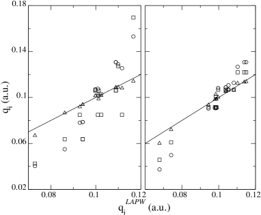
Figure 9: Charge excesses on Cu sites $q_{i}$ for the same $Cu_{0.50}Zn_{0.50}$ alloys as in Fig. 8. Circles, triangles and squares represent the calculated values by CEF-PCPA, CEF-LAPW and by the model of Ref. Magri et al., 1990, In abscissa the charge excesses obtained by LAPW calculations are reported. Left frame: bcc-based alloys; right frame: fcc-based alloys. In oder to improve readability we plot also the straight lines $q=q^{LAPW}$. The deviations from these lines measure the accuracy of the various calculations.

Interestingly, the present CEF-LAPW calculations confirm the observations about the transferability of CEF parameters in Ref. Bruno et al., 2003, where the CEF charges have been compared vs. LSMS results. As a typical example, let us consider the results for $c=0.50$ reported in Table 3. The $<\Delta q^{2}>$ obtained are alway small: $4\;10^{-5}$ in the worst case and $4\;10^{-7}$ in the best, corresponding respectively to structures 71 and 74, while an intermediate value, $3\;10^{-6}$ is found for the structure $R16$, from which the CEF-LAPW coefficients have been obtained. The same holds for all the concentrations, both for bcc and fcc structures. A look to the columns (c) in the Tables 3 and 4, in fact, shows that while excellent results have been obtained for all the supercell, the random structure from which the CEF coefficients have been extracted is not necessarily the best performing.

The above arguments about the charges should not lead to the conclusion that, for this purpose, any fit is comparable with any other. This is clearly shown in Fig. 9, where the performances of PCPA, CEF-PCPA, CEF-LAPW and by the model of Magri et al. Magri et al. (1990) are compared for the equiatomic concentration alloys. In the same Figure, the distances from the diagonal lines measures the differences between the LAPW charges and those by various approximations, for all the Cu sites in the supercells with $c=0.5$. It is there evident that the results by CEF-LAPW, marked by open triangles, are much better than those by other approximations.

IV.2 Total energies

In Tables 3 and 4 we compare the total energies obtained for CuZn alloys by CEF, PCPA and LAPW calculations. We have used the same extended set of bcc and fcc based structures listed in Ref. Curtarolo, 2003. Since the CEF energies contain a, concentration dependent constant, we report the quantity $\Delta E$, defined as the energy difference between the structure at hand and the structure that, at the same concentration, has the lowest energy, according with PCPA calculations. The same $\Delta E$ is plotted in Figs. 10 and 11 for the Cu concentrations $c=0.25$, $0.50$, an $0.75$, for which the database of Ref. Curtarolo, 2003 contains a number of structure sufficient to individuate trends.

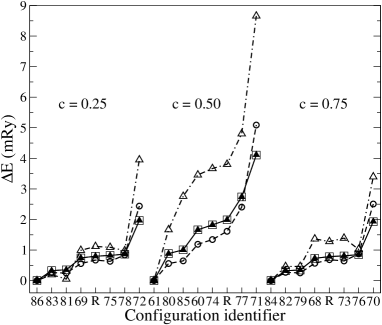
Figure 10: Total energy differences with respect to the PCPA predicted ground state, $\Delta E$, for bcc based Cu_cZn_1-c alloys. The labels indicated in abscissa identify the various configurations in the database of Ref. Curtarolo, 2003, $R$ stands for structures with randomly generated chemical occupations containing 16 atoms with mean Cu contents c=0.25, 0.5 and 0.75. Open triangles, open circles, open squares and filled triangles, indicate LAPW, CEF-LAPW, CEF-PCPA and PCPA calculations, respectively. Lines are a guide for the eye.

Our first observation is that the total energies obtained by PCPA and CEF-PCPA calculations perfectly overlap on the scale of Figs. 10 and 11, where they are represented as filled triangles and open squares, respectively. As reported in Tables 3 and 4, in fact, the values obtained by the two methods are different by a few $\mu Ry$ per atom, that is comparable with the accuracy of the calculations. Thus, PCPA and CEF-PCPA give indintinguishable results both for the charges (as discussed in the previous subsection) and the total energies. Therefore, it is compelling to conclude that the CEF theory is a numerically excellent and powerful tool to reproduce with much less efforts GCPA electronic structure calculations. Moreover, since CEF-PCPA calculations use as an input the ’qV’ data obtained from random supercells, the perfect agreement obtained for the properties of so many different ordered structures that have not been used to fit the CEF coefficients has only one possible explanation. Accordingly with the discussion in Sects. III B and III C, both the following conditions must be fulfilled. (i) The coherent scattering-path matrix $\underline{\tau}^{c}$ of the random alloy configuration used as an input must be representative of the whole set of ordered structures considered; (ii) the linearity of the ’qV’ laws is almost perfectly observed in all the range of values that the charge excesses and the Madelung potentials take for the structures considered. In Sect. III we have offered several arguments supporting the validity of both points above, but we have not been able to provide an analytical demonstration. We think that the numerical evidence found is very strong and compelling.

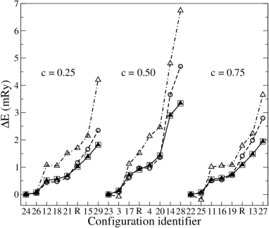
Figure 11: Total energy differences with respect to the PCPA predicted ground state, $\Delta E$, for fcc based Cu_cZn_1-c alloys. The labels indicated in abscissa identify the various configurations in the database of Ref. Curtarolo, 2003, $R$ stands for structures with randomly generated chemical occupations containing 16 atoms with mean Cu contents c=0.25, 0.5 and 0.75. Open triangles, open circles, open squares and filled triangles, indicate LAPW, CEF-LAPW, CEF-PCPA and PCPA calculations, respectively. Lines are a guide for the eye.

Accordingly with the discussion in Sect. III, the success of the CEF theory in reproducing the charges or, equivalently, the Madelung potentials guarantees the reproducibility of any ground state property within the GCPA theory through Eq. (41). Hence, even spectral properties as the DOS or the Bloch Spectral functions, although buried, are contained in the CEF functional that, if the input parameters are extracted from a GCPA theory, inherits all the good and the bad things of same GCPA theory.

The comparison with LAPW calculations is more difficult, for two different reasons. In first place, these calculations do not assume mean boundary conditions for the wave-functions and use a procedure equivalent to the full calculation of the $\underline{\underline{\tau}}$ matrix. In second place, within LAPW calculations, the charge multipole summation is truncated at some high $\ell$ value. With these clarifications, the agreement between LAPW and PCPA or CEF-PCPA calculations (there is no reason for discussing the last two models separately) is quite good. As a general rule, the two set of calculations find the same ground states at the concentrations considered. In the few exceptions (that correspond to the negative figures in the LAPW columns of Tables 3 and 4) the disagreement can be explained by the fact that the structures indicated as the ground state by the two theories are almost degenerate in energy. Also the general trends for the total energies are well reproduced, as it is visible in Figs. 10 and 11, though the PCPA generally underestimate the energy differences.

Fitting the CEF parameters from the LAPW ’qV’ laws generally improves the agreement. At variance of what found for the charges, however, the improvement is quite modest.

In summary: the CEF appears able to perfectly reproduce GCPA calculations for both ordered and disordered metallic systems. The reasons why the agreement is so excellent are not yet completely understood. Although CEF and GCPA theories are both coarse grained versions of the DFT, opposite to what numerical results suggest, they are not the same theory. In fact, as discussed in Sect. III, in order to be coincident to the CEF, GCPA theories should (i) exactly observe linear ’qV’ laws and (ii) lead to coherent scattering matrices independent on the configuration in a fixed concentration ensemble. For metallic alloys, these conditions appear plausible and the numerical evidence strongly support the view that both are nearly satisfied. However we must highlight that the condition (i) is not verified for pathologically high values of the Madelung field. The comparison vs. LAPW calculations suggest that both coarse grained theories, GCPA and CEF, are able to reproduce semiquantitatively the total energies of the alloy configurations considered. In particular, the results by the coarse grained theories are strongly correlated with those by LAPW. This fact is better elucidated by Figs. 10 and 11, where configurations belonging to the same fixed concentration ensemble are ordered in such a way to have increasing PCPA total energies. If the same ordering was not observed by some other method for some configuration, this would show up as a local minimum in the corresponding curve. The most visible of such events, occurs in Fig. 11 for $c=0.75$, where the curve corresponding to LAPW calculations presents a very weak local minimum at the configuration 25. The examination of Figs. 10 and 11 suggests that the coarse grained theories are able to give qualitatively correct predictions about ordering for the alloys considered, while the fact that they generally underestimate the corresponding energies could imply incorrect estimates of the corresponding transition temperatures.

V Conclusions

We wish to conclude this paper with a summary and a few comments.

We have introduced the class of the GCPA theories, that are characterized by (i) a specific ansatz for the kinetic part of the density functional, which is common to all CPA-based theories, and (ii) an external model that determines the way in which the atomic effective potentials should be reconstructed and the statistical weights to be assigned each. The GCPA class of approximations includes most existing CPA-based density functional theories, to mention a few: the CPA prototype, i.e. the single site CPA Johnson et al. (1986, 1990), the Screened Impurity Model CPA (SIM-CPA) Abrikosov et al. (1991, 1992), the Polymorphous CPA (PCPA) Ujfalussy et al. (2000), the CPA including Local Fields (CPA+LF) Bruno et al. (2002), the Non Local CPA (NL-CPA) Rowlands et al. (2003). The ansatz (i) consists in applying averaged boundary conditions at the surfaces of each scattering volume and naturally leads to algorithms requiring a number of operation that scales as $N$. As it is discussed by Abrikosov and Johansson Abrikosov and Johansson (1998), CPA-based approximations allow for a careful picture of the spectral properties of metallic alloys. The so much criticized results of the SS-CPA about the total alloy energies can be healed by external models that consider the charge distribution in the system. We have shown how this can be done systematically by writing the relevant energetic contributions as a series involving the charge multipole moments in each scattering volume. The truncation errors of the same series are probably already quite small when only the first term is included, as in the case of spherical approximations.

We have derived an expression of the GCPA density functional that, together with the above multipole sums, includes local ’atomic’ terms, completely determined by the atomic number of the ion in the volume, and by the geometry of the same volume. The local term at the $i$-th site is coupled to the others only through the coherent scattering matrix $\underline{\tau}^{c}$ and the Madelung potential at the same site. Although this kind of coupling, that we have called marginal coupling, is not necessarily weak, nevertheless, it is analytically tractable and it is the source of the $O(N)$ scaling in GCPA theories. We have demonstrated that in a GCPA theory all ground state properties within a specific sample are functions of the appropriate coupling Madelung potential only, or, equivalently, of the charge multipole moments at each lattice site. To put it into other words: we have demonstrated that the GCPA approximations realize a coarse graining of the Hohenberg-Kohn density functional, since only a part of the information conveyed by the electronic density field, namely the charge multipole moments, is actually entering in the GCPA approximate functional. Moreover we have suggested that the explicit form of the GCPA functional dependence on the multipole moments can be obtained in a fixed concentration ensemble by the numerical integration of the ’qV’ relationships for a random alloy configuration belonging to the same ensemble. The above procedure does not rely on the linearity of the ’qV’ laws.

We have re-derived the CEF Bruno et al. (2003) as a sensible approximation of the GCPA theories, with which it would coincide provided the ’qV’ were exactly linear as claimed by many groups. The present derivation allows for the inclusion of higher order multipole moments. A very remarkable feature of the CEF theory is that it shares the same structure of the MST. In fact, the minimization of the CEF requires the solution of a set of Euler-Lagrange equations that has the same structure of the Korringa-Kohn-Rostoker (KKR) matrix at zero energy and wave-vector Bruno (2007); Drchal et al. (2006). More specifically, as it can be seen by comparing Eqs. (4) and (52), the site-diagonal response functions, $a_{i,LL^{\prime}}$, and the Madelung coefficients, $M_{ij,LL^{\prime}}$, in the CEF theory, play the role of the site diagonal scattering matrices and the KKR structure constants in the MST theory. The correspondence is not only formal, since the $a_{i,LL^{\prime}}$ are single-site quantities in the same sense of the SS scattering matrices Bruno (2007) and, in plain analogy with them, are related with the SS response to the appropriate perturbing field Bruno et al. (2002).

In the present paper we have provided several formal arguments and strong numerical evidences that CEF and GCPA theories lead to very similar results, the discrepancies being of the order of the numerical errors. We have also shown that CEF and GCPA theories are able to reproduce the charges and the total energies for many ordered alloy configurations. In our view the coarse grained theories, GCPA and CEF, constitute a valuable alternative to full DFT calculations.

Although the CPA theory was proposed many year ago with the purpose of dealing with substitutionally disordered alloys, we think that we have shown that today GCPA theories are able to deal with ordered intermetallic compounds too. Therefore, the fact that CPA-based theories are able to cope with sophisticated model of disorder is not an original sin but, rather, an added value.

The computational performances of the CEF have been discussed in more details elsewhere Bruno et al. (2003). Here we like to mention that the possibility of evaluating total energies for thousand atoms in a few seconds CPU time could constitute a substantial enlargement of the domain of the applications of the DFT.