Analytic results on long-distance entanglement mediated by gapped spin chains

Abstract

Recent numerical results showed that spin chains are able to produce long-distance entanglement (LDE). We develop a formalism that allows the computation of LDE for weakly interacting probes with gapped many-body systems. At zero temperature, a dc response function determines the ability of the physical system to generate genuine quantum correlations between the probes. We show that the biquadratic Heisenberg spin-1 chain is able to produce LDE in the thermodynamic limit and that the finite antiferromagnetic Heisenberg chain maximally entangles two spin-$1/2$ probes very far apart. These results support the current perspective of using quantum spin chains as entanglers or quantum channels in quantum information devices.

The quantum information (QI) approach of regarding entanglement as a information resource (NMA00, ) stimulated important developments in its characterization and in ways to measure it. On the other hand, in condensed matter physics, quantum correlations have long been recognized as an essential ingredient in many low-temperature phases. These facts lead to a considerable amount of work on the characterization of the entanglement properties of many-body systems at zero temperatures (for reviews see (ALFR, )), particularly near quantum phase transitions and also at finite temperatures (ON, ; VMC, ; Ved, ).

Feasible mechanisms of entanglement extraction from real solid state (DCG06, ) and their ability to transfer entanglement between distant parties (PMB05, ) are of crucial importance for the implementation of QI protocols, such as teleportation or superdense coding. In systems with short-range interactions, though, entanglement between two particles usually decays quickly with distance between them (ON, ). However, Campos Venuti et al (VBR06, ), have recently found, in numerical density matrix renormalization (DMRG) studies, that certain correlated spin chains are able to establish long-distance entanglement (LDE) between probes to which they couple, without the need of an optimal measurement strategy onto the rest of the spins (VMC, ). This naturally raises the question of which classes of strongly correlated systems are able to produce LDE.

In this paper, we present a quantitative description of the effective Hamiltonian of interaction between probes weakly coupled to gapped many-body systems. This allows us to confirm some of the numerical evidence of LDE found by DMRG (VBR06, ) and to obtain new results concerning two important spin chain models. Although our formalism can be applied to general gapped many-body systems, here we focus on one-dimensional spin chains. In the spirit of (VBR06, ), two probes, $a$ and $b$, interact with the spin chain, locally, through sites $m$ and $n$, respectively. The Hamiltonian of the system reads $H=H_{0}+V_{m,n}$, where $H_{0}$ is the full many-body Hamiltonian of the spin chain and $V_{m,n}=V_{a,m}+V_{b,n}$ describes the interaction between the probes and the spin chain. We will show that, as long as the probes interact weakly with the many-body system, the ground state (g.s.) of the full system may display LDE between the probes, i.e., $E(\rho_{ab})>0$ when $|m-n|$ is of the order of the system size. The opposite limit, i.e., strong interactions, will cause the probes to develop robust correlations with the site they interact inhibiting entanglement with them (VBR06, ). This arises from a constraint on the correlations between different sub-systems known as the monogamy of entanglement (CKW00, ). In order to maximize the spin chain potential to entangle the probes, we require that $J_{p}\ll J$, where $J_{p}$ is the interaction strength between the probes ($a,b$) and the spins at $m$ and $n$, and $J$ is a typical energy scale for the spin system (for instance, a nearest-neighbor exchange interaction). For $J_{p}=0$ the state of the probes becomes totally uncorrelated and the g.s. of the entire system becomes ($d\times d$)-fold-degenerate. In this case we may write $|\psi\rangle=|\psi_{0}\rangle\otimes|\chi_{a}\rangle\otimes|\chi_{b}\rangle$, where $|\psi_{0}\rangle$ is the g.s. of the spin chain (assumed non-degenerate) and $|\chi_{\gamma}\rangle$ the state of the probe $\gamma$. The role of the interaction ($J_{p}>0$) is to lift this degeneracy causing the probes to develop correlations. For weak coupling $J_{p}$, the effective Hamiltonian in this $d\times d$ low-energy subspace, obtained as discussed below, will determine the dynamics and correlations of the probes. For the special case of spin one-half probes ($d=2$), the negativity (Vidal02, ), or any other equivalent entanglement monotone, can be used to quantify the entanglement.

The effective Hamiltonian. In a very general way we can write the local interaction between the probes and the corresponding sites in the many-body system in the following manner:

$$V=\sum_{\alpha=1}^{p}\gamma_{\alpha}^{a}O_{m}^{\alpha}\otimes A^{\alpha}\otimes\openone_{b}+\gamma_{\beta}^{b}O_{n}^{\alpha}\otimes\openone_{a}\otimes B^{\alpha},$$ (1)

where $A^{\alpha}$$(B^{\alpha})$ denotes an operator acting on the Hilbert space of the probe $a(b)$ and $\openone_{a(b)}$ the corresponding identity operators. The many-body system operators on sites $m$ are represented by $O_{m}^{\alpha}$ and $\gamma_{\alpha}^{a(b)}$ is the coupling strength. The projector onto the states with unperturbed energy $E_{0}\equiv\langle\psi|H_{0}|\psi\rangle$ is $\mathcal{P}_{0}=|\psi_{0}\rangle\langle\psi_{0}|\otimes\openone_{a}\otimes\openone_{b}.$ Let $\mathcal{P}_{k}$ ($k>0)$ be the projector onto the subspace of energy $E_{k}>E_{0}$ , so that $\openone=\mathcal{P}_{0}+\sum_{k>0}\mathcal{P}_{k}$. Using the standard canonical transformation formalism (SW66, ) one can determine probes g.s. by diagonalizing an effective Hamiltonian in the subspace spanned by $\mathcal{P}_{0}$, namely, $H_{eff}=\mathcal{P}_{0}(H_{0}+V)\mathcal{P}_{0}+|\psi_{0}\rangle\langle\psi_{0}|\otimes H^{(ab)}$ (NOTE, ). This a familiar concept that finds many applications in condensed matter physics, such as, for instance, in the derivation of the Ruderman-Kittel-Kasuya-Yosida magnetic interaction between local moments in a metal (KAS56b, ). The coupling between the probes is given by $H^{(ab)}=-\sum_{k>0}\langle UP_{k}U\rangle_{0}(E_{k}-E_{0})^{-1},$ where the average is taken with respect to the g.s. of the spin chain $\langle UP_{k}U\rangle_{0}=\langle\psi_{0}|UP_{k}U|\psi_{0}\rangle$ and $U:=V-\langle V\rangle_{0}$. Note that, by definition, $\langle U\rangle_{0}=\mathcal{P}_{0}U\mathcal{P}_{0}=0$. Entanglement between the probes arises from $H^{(ab)}$ since it contains nonlocal terms such as $U_{a,m}\mathcal{P}_{k}U_{b,n}$ (Li, ). The probe Hamiltonian can be transformed by straightforward manipulations into an explicit form involving time dependent correlation functions of the spin chain. A similar procedure is used to express cross sections of scattering by many-body systems in terms of its correlation functions (Squ78, ). We obtain (we set $\hbar=1$, see (Correlation, ) for the derivation)

$$H^{(ab)}=-\frac{1}{2\pi}\int_{-\infty}^{+\infty}\frac{dE}{E}\int_{-\infty}^{+\infty}dt\langle U(t)U\rangle_{0}e^{iEt}.$$

We now introduce the explicit form of $U$ to arrive at the desired result $H^{(ab)}=H_{L}^{(a)}+H_{L}^{(b)}+H_{NL}^{(ab)}+H_{L}^{(ab)},$ (see (Local, ) for a comment on the local terms). Defining the two-body connected correlation $\langle O_{m}^{\alpha}(t)O_{n}^{\beta}\rangle_{c}=\langle\psi_{0}|O_{m}^{\alpha}(t)O_{n}^{\beta}|\psi_{0}\rangle-\langle\psi_{0}|O_{m}^{\alpha}(t)|\psi_{0}\rangle\langle\psi_{0}|O_{n}^{\beta}|\psi_{0}\rangle$ the term coupling the two probes yields

$$H_{NL}^{(ab)} = \sum_{\alpha,\beta=1}^{p}\gamma_{\alpha}^{a}\gamma_{\beta}^{b}(C_{m\alpha;n\beta}+C_{n\beta;m\alpha})A^{\alpha}\otimes B^{\beta},$$ (2)

$$C_{m\alpha;n\beta} = \frac{1}{2i}\int_{-\infty}^{\infty}{dte^{-0^{+}|t|}sign(t)\langle O_{m}^{\alpha}(t)O_{n}^{\beta}(0)\rangle_{c}}.$$ (3)

The coupling between the probes can be expressed in terms of the response function $\chi_{m\alpha;n\beta}(t)=-i\langle[O_{m}^{\alpha}(t),O_{n}^{\beta}]\rangle\theta(t)$, where $\theta(t)$ is the Heaviside step function. Using the Lehman representation at $T=0$ one can show that

$$\tilde{\chi}{}_{m\alpha;n\beta}(0) = C_{m\alpha;n\beta}+C_{n\beta;m\alpha},$$

where $\tilde{\chi}_{m\alpha;n\beta}(\omega)$ is the time Fourier transform of $\chi_{m\alpha;n\beta}(t)$. The effective Hamiltonian Eq. (2) lifts the degeneracy of the GS level of the uncoupled system ($J_{p}=0$). As long as the couplings appearing in $H_{NL}^{(ab)}$ are small compared to typical energy scales of the spin chain, such as the gap to first excited state, $\Delta$, the low-energy physics of this system, $E\ll\Delta$, with no real excitations of the spin chain, will be well described by $H_{NL}^{(ab)}$. This condition limits the strength of the chain-probe interaction, but is shown by numerical results to be the appropriate limit to maximize LDE (VBR06, ).

In the remainder of the paper we will compute the LDE for two rotational invariant spin chains: the finite Heisenberg spin-$1/2$ chain in zero field using the exact results from bosonization theory; a specific spin-1 Heisenberg chain with biquadratic interactions by means of a approximation scheme for its spectrum. It is useful to write Eq. (1) in terms of spin operators $\vec{S}_{m}$ for the spin chain and $\vec{\tau}_{a(b)}$ for the probes. Considering that the probes couple with the spin chain via an Heisenberg interaction, the most common situation, $V_{m,n}=J_{a}\vec{S}_{m}\cdot\vec{\tau}_{a}+J_{b}\vec{S_{n}}\cdot\vec{\tau}_{b}$, the connection with the previous notation becomes straightforward: $O_{m}^{\alpha}=S_{m}^{\alpha}$, $A^{\alpha}(B^{\alpha})=\tau_{a(b)}^{\alpha}$ and $\gamma_{\alpha}^{a(b)}=J_{a(b)}$. Eq. (2) becomes simply,

$$H_{eff}=J_{ab}\vec{\tau}_{a}\cdot\vec{\tau}_{b},$$ (4)

where $J_{ab}=J_{a}J_{b}\tilde{\chi}{}_{m\alpha;n\alpha}(0)$ and $\alpha=x$, $y$ or $z$.

The finite antiferromagnetic Heisenberg spin-$1/2$ chain. The isotropic antiferromagnetic Heisenberg model reads

$$H:=\sum_{i=1}^{L-1}\vec{S}_{i}\cdot\vec{S}_{i+1}.$$ (5)

Our formalism only applies to the finite chain which has gapped excitations. To calculate its time-dependent correlation functions we will use the conformal invariance of the critical infinite chain ($L\rightarrow\infty$). We show below that its time-dependent correlations are enough to extract the effective coupling $J_{ab}$ for the finite chain. It is clear that the effective Hamiltonian Eq. (2) will preserve the full SU(2) symmetry of the interaction Hamiltonian $H+V_{m,n}$, i.e. no local terms will give contribution to $H_{eff}$. Assuming that the probes couple to the spin chain with the same strength ($J_{a}=J_{b}\equiv J_{p}$), $H_{eff}$ takes the very compact form

$$H_{eff}=J_{p}^{2}\tilde{\chi}_{m\alpha;n\alpha}(0)\vec{\tau}_{a}\cdot\vec{\tau}_{b}.$$ (6)

Hence, whenever $\tilde{\chi}_{m\alpha;n\alpha}(0)>0$ the g.s. of the probes is a singlet-state displaying maximal LDE (remark, ). Our computation of $\tilde{\chi}_{m\alpha;n\alpha}(0)$ will rely on general bosonization results for correlations of spin-1/2 chains (see (TG04, ) for a review) and the conformal invariance of the critical chain. The dominant long-distance correlations of the g.s. of Hamiltonian Eq. (5) oscillate with a $\pi$ phase change between neighbor spins. It is therefore useful to define the retarded Green function for the staggered magnetization $M_{j}^{\alpha}:=(-1)^{j}S_{j}^{\alpha}$, $G_{mn}^{R}(t):=i\langle[M_{m}^{\alpha},M_{n}^{\alpha}(t)]\rangle\theta(t)$. The response function in Eq. (6) is $\chi{}_{m\alpha;n\alpha}(t)=(-1)^{|m-n|}G_{mn}^{R}(t)$. The retarded Green function is obtained from the corresponding Matsubara Green function, $G(x,\tau):=\langle\hat{T}_{\tau}M_{m}^{\alpha}(x_{m},\tau)M_{n}^{\alpha}(x_{n},0)\rangle$, with imaginary time $\tau\in[-\beta,\beta]$ and where, in the limit $|x_{m}-x_{n}|\gg 1$, we may replace $x_{m}-x_{n}$ by a continuum variable $x$. The Matsubara Green function for the infinite chain reads (SAC99, )

$$G(x,\tau)=\mathcal{A}|v_{F}\tau+\imath x|^{-1};$$

$\mathcal{A}$ is an amplitude and $v_{F}$ the Fermi velocity of the spinon excitations. This result implies that the infinite chain has a divergent $\tilde{\chi}_{m\alpha;n\alpha}(0)$; this is a direct consequence of a zero gap and a signal of the critical nature of the spin chain at $T=0$. Nevertheless, the finite chain is gapped, has a finite $\tilde{\chi}_{m\alpha;n\alpha}(0)$, and the above result can be used to calculate its correlation functions, precisely because the critical nature of the infinite chain implies that $N$-point correlation functions in different geometries are related by conformal transformations (Conformal, ). The mapping of the infinite chain to the finite chain is achieved by the following analytic transformation (see Fig. 1), $w=\frac{L}{2\pi}\ln z=u+\imath r,$ where $z=v_{F}\tau+\imath x$.

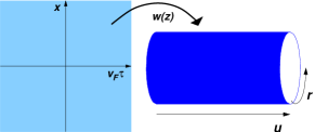
Figure 1: The conformal transformation $w(z)=u+\imath r$ maps every point $(v_{F}\tau,x)$ in the plane into the strip geometry ($u\in]-\infty,\infty[$, $r\in[-L/2,L/2]$) with periodic boundary conditions along the $v$ direction.

Using the transformation law for conformal invariant theories (Conformal, ) the Matsubara Green function for the finite antiferromagnetic Heisenberg chain with periodic boundary conditions in the spatial coordinate $r$ reads (Cardy, ) $G_{cyl}(r,u)=2\pi\frac{\mathcal{A}}{L}(2\cosh(2\pi u/L)-2\cos(2\pi r/L))^{-\frac{1}{2}}.$The analytic continuation to real time is made by Wick rotation $u\rightarrow\imath v_{F}t+0^{+}sgn(t)$ and the corresponding retarded Green function defined in the cylinder $G_{cyl}^{R}(r,t)$ can be computed from the time-ordered Green function $G^{R}(r,t)=-2\theta(t)\Im\left[G(r,t)\right]$(see (TG04, )). Setting the branch cut of the logarithm in the negative real axis we find

$$G_{cyl}^{R}(r,t)=2\pi\frac{\mathcal{A}}{L}\frac{\theta(t)\theta(F(r,t))sign(\sin(2\pi t/L))}{\sqrt{F(r,t)}},$$

where $F(r,t)=2\cos(2\pi r/L)-2\cos(2\pi t/L)$. The response function at zero frequency is then given by $\tilde{\chi}_{m\alpha;n\alpha}(0)=(-1)^{|m-n|}\int_{0}^{\infty}dtG^{R}(r,t)\exp(-0^{+}t$). Here we only state the result,

$$\tilde{\chi}_{m\alpha;n\alpha}(0)=\mathcal{C}_{mn}\int_{2\pi r/L}^{\pi}dy\frac{y/\pi-1}{\sqrt{\cos(2\pi r/L)-\cos(y)}},$$

with $\mathcal{C}_{mn}=(-1)^{|m-n|}\mathcal{A}/(2v_{F})$. Figure 2 shows the plot of the absolute value of the response function at zero frequency confirming the existence of LDE for a wide range of values of $r/L$. Note that $\tilde{\chi}_{m\alpha;n\alpha}(0)$ diverges logarithmically at the origin. Our perturbative approach cannot be applied unless $J_{p}^{2}\tilde{\chi}_{m\alpha;n\alpha}(0)\ll\Delta\sim J/L$, and will fail in the thermodynamic limit ($L\to\infty$) for fixed $r$. The numerical results of Ref. (VBR06, ) show probes almost completely entangled only for small values of $J_{p}\sim 0.1$, for a finite chain $L=26$. This value is well estimated by the limit of validity of our perturbative approach, for $r/L\sim O(1)$, namely, $J_{p}\ll J/\sqrt{L}$. These results, in the light of our analysis, strongly suggest that the conditions for LDE are coincident with the conditions for validity of the perturbative approach. Weakly coupled probes get maximally entangled by the effective antiferromagnetic interaction mediated by the spin chain.

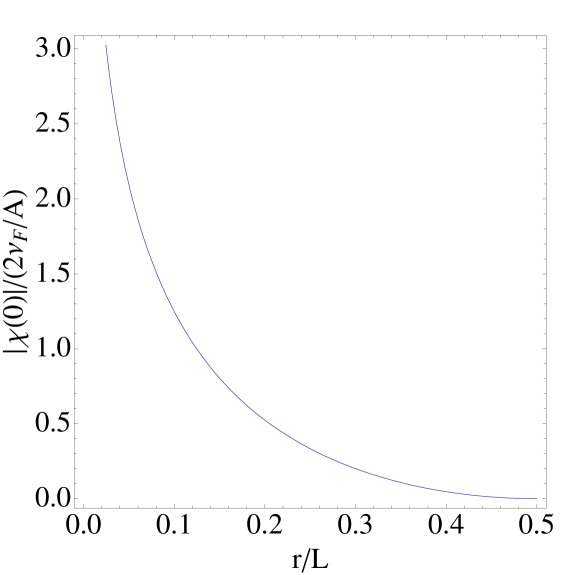
Figure 2: The absolute value of the response function at zero frequency for the finite antiferromagnetic Heisenberg chain. We have assumed $r\gg 1$ so that the results from bosonization theory are accurate.

The AKLT model. The Heisenberg spin one-chain with biquadratic interactions reads

$$H:=\sum_{i=1}^{N-1}\left[\vec{S}_{i}\cdot\vec{S}_{i+1}+\beta(\vec{S}_{i}\cdot\vec{S}_{i+1})^{2}\right].$$

This model admits an exact solution for $\beta=1/3$ which is known as the Affleck-Kennedy-Lieb-Tasaki (AKLT) point (AKL+88, ). A picture of the g.s. is given by the so-called valence-bond-solid (VBS). Each spin-1 is represented by a couple of spins one-half, as long as the antisymmetric state is projected out. The VBS state is constructed by forming short-ranged singlets between nearest spin-$1/2$ and then symmetrizing local pairs to get back $S=1$ states. In the thermodynamic limit, the static correlations are very short-ranged [$\xi_{AKLT}=1/ln(3)\cong 0.9$] (AKL+88, ). For this reason we may ask whether two probes are able to get entangled by interaction mediated by the spin-$1$ chain. We cannot make an exact computation of LDE as in the Heisenberg model, since the exact dynamical correlations are not known even for large distances. However, as suggested by Arovas et al (ADP88, ), we can apply the single-mode approximation (SMA) used to deduce the phonon-roton curve in liquid 4He (FRP72, ), in order to study the excitations in this model. This is done by assuming that a excited state at wave vector $q$ is given by

$$|q\rangle\equiv S_{q}^{z}|\psi_{0}\rangle=N^{-1/2}\sum_{i}e^{\imath qr_{i}}S_{i}^{z}|\psi_{0}\rangle,$$

where $|\psi_{0}\rangle$ is the exact g.s. of the AKLT model. Within the SMA the dynamical structure factor $\mathcal{S}^{\alpha\beta}$ is related with the static structure factor defined as $s^{\alpha\beta}(q)=\langle\psi_{0}|S_{-q}^{\alpha}S_{q}^{\beta}|\psi_{0}\rangle$ in the simple way $\mathcal{S}(q,w)\cong s(q)\delta(w-w_{q})$. In (ADP88, ) it was shown that, $w_{q}=E_{q}-E_{0}=5(5+3\cos q)/27$ and that $s(q)=(10/27)(1-\cos q)/w_{q}$. The knowledge of the dynamical structure factor allows us to compute the effective couplings of Eq. (2) by inverse Fourier transform. For the AKLT model we obtain

$$\tilde{\chi}_{m+r\alpha;m\alpha}(0)=\int_{0}^{\infty}\frac{dt}{2\pi}\int_{-\pi}^{\pi}dq\cos(qr)\sin(w_{q}t)(a+\frac{b}{w_{q}})$$

with $a=-2/3$, $b=80/81$. These integrals may be done by defining $f(t)=\sin(w_{q}t)\theta(t)$ and noting that $\gamma=\int_{-\infty}^{\infty}dt\sin(w_{q}t)\theta(t)=\hat{f}(w=0)$ where $\hat{f}(w)$ is the Fourier transform of $f(t)$. We obtain $2\hat{f}(w)=(w+w_{q}-i0^{+})^{-1}-(w-w_{q}-i0^{+})^{-1}$ and $\gamma=1/w_{q}$. The remaining integral is done by extending the integrand to the complex plain and computing the residues. This yields, $J_{ab}=-\frac{27}{10}J_{p}^{2}(-1)^{r}(1+\frac{4}{3}r)e^{-\frac{r}{\xi_{AKLT}}}$. The sign of the interaction mediated by the AKLT spin chain changes according to the distance between the probes. This comes from the fact that the static correlations in this spin chain have a similar alternation. Therefore at $T=0$ the probes get entangled whenever their distance corresponds to a odd number of sites.

The effect of finite temperature and final comments. If the temperature is such that $k_{B}T\ll\Delta$, we do not expect real excitations of the spin chain to be present. Only the subspace of states described by $\hat{H}_{eff}$ will be populated and we may calculate the correlations between the probes using $\rho_{ab}=e^{-\beta\hat{H}_{eff}}/Tr[e^{-\beta\hat{H}_{eff}}]$ with $\beta^{-1}=k_{B}T$. This defines a temperature, $1/\beta^{*}$, above which entanglement disappears. For an antiferromagnetic $\hat{H}_{eff}$ the computation of the negativity yields $\beta^{*}J_{mn}\simeq 0.27$. Loosely speaking, the probes will be entangled whenever the temperature is smaller than the effective coupling between the probes. This formalism has also been used to discuss qubit teleportation and state transfer across spin chains (VBR06, ). In conclusion, we have expressed the capacity of a gapped many-body system as an entangler of weakly coupled probes at arbitrary distances in terms of a zero temperature response function. We exemplified this formalism by calculating this function for two quantum spin chains, shedding light on recent numerical results on LDE. In this context, our results strongly suggest that the main mechanism of LDE mediated by gapped spin chains is the existence of dominant antiferromagnetic correlations. Acknowledgments. We gratefully acknowledge very enlightening discussions with J. Penedones. A.F. was supported by FCT (Portugal) through PRAXIS Grant No. SFRH/BD/18292/04.

References

- (1) M. A. Nielsen and I. L. Chuang, Quantum Computation and Quantum Information (Cambridge University Press, Cambridge, 2000).
- (2) L. Amico, R. Fazio, A. Osterloh and Vedral, e-print arXiv:quantum-ph/070344v1 (2007); J. I. Latorre, E.Rico and G. Vidal, Quant. Inf. Comput. 4, 48 (2004).
- (3) T. J. Osborne and M. A. Nielsen, Phys. Rev. A 66, 032110 (2000); A. Osterloh, L. Amico, G. Falci, and R. Fazio, Nature (London) 416, 606 (2002).
- (4) F. Verstraete, M. A. Martín-Delgado, and J. I. Cirac, Phys. Rev. Lett. 92, 087201 (2004).
- (5) V. Vedral, New. J. Phys. 6, 102 (2004).
- (6) G. De Chiara et al, New. J. Phys. 8, 95 (2006).
- (7) M. B. Plenio and F. L. Semião, New. J. Phys. 7, 73 (2005); M. J. Hartmann, M. E. Reuter, and M. B. Plenio, ibid. 8, 94 (2004).
- (8) L. Campos Venuti, C. Degli Esposti Boschi, and M. Roncaglia, Phys. Rev. Lett. 96 247206 (2006); ibid. 99 060401 (2007).
- (9) V. Coffman, J. Kundu, and W. K. Wootters, Phys. Rev. A 61, 052306 (2000).
- (10) G. Vidal and R. R. Werner, Phys. Rev. A 65, 032314 (2002).
- (11) J. R. Schrieffer and P. A. Wolff, Phys. Rev. 149, 491 (1966).
- (12) contributes with a constant, and thus will be set to zero as it does not change the eigenstates.
- (13) T. Kasuya, Prog. Theor. Phys. 16, 45 and 58 (1956); M. A. Ruderman and C. Kittel, Phys. Rev. 96, 99 (1954); K. Yosida, ibid. 106, 893 (1957).
- (14) Y. Li et al, Phys. Rev. A 71, 022301 (2005).
- (15) We rewrite as and use the integral representation of the Dirac delta function, and the fact that where is the probe-spin-chain coupling in the Heisenberg representation for the spin chain. Finally we can set to our advantage, by including the term in the sum over and, since , we obtain the stated result.
- (16) The local terms in read and . These terms are either constants or zero in the cases we consider.
- (17) More precisely, due to the perturbative nature of our formalism with expansion parameter , the negativity or any other entanglement monotone will deviate from the value of maximal entanglement (the singlet state) with corrections of the order of , which are negligible for weakly interacting probes, i.e. .
- (18) T. Giamarchi, Quantum Physics in One Dimension (Clarendon Press, Oxford, 2004).
- (19) S. Sachdev, Quantum Phase Transitions (Cambridge University Press, Cambridge, 1999).
- (20) In a conformally invariant two-dimensional system with scaling dimension the 2-point correlation function has the transformation law generated by any analytic function . The subscripts and refer to the boundary geometry where the theory is defined.
- (21) J. L. Cardy, J. Phys. A: Math. Gen. 17, L385 (1984).
- (22) I. Affleck, T. Kennedy, E. H. Lieb, and H. Tasaki, Commun. Math. Phys. 115, 477 (1988).
- (23) G. L. Squires, Introduction to the theory of thermal neutron scattering (Cambridge University Press, Cambridge, 1978).
- (24) D. P. Arovas, A. Auerbach, and F. D. M. Haldane, Phys. Rev. Lett. 60, 531 (1988).
- (25) R. P. Feynman, Statistical Mechanics, (Benjamim, New York, 1985); S. M. Girvin, A. H. MacDonald, and P. M. Platzman, Phys. Rev. Lett. 54, 581 (1985).