Solar Cycle Variation of Real CME Latitudes

Abstract

With the assumption of radial motion and uniform longitudinal distribution of coronal mass ejections (CMEs), we propose a method to eliminate projection effects from the apparent observed CME latitude distribution. This method has been applied to SOHO LASCO data from 1996 January to 2006 December. As a result, we find that the real CME latitude distribution had the following characteristics: (1) High-latitude CMEs ($\theta>60^{\circ}$ where $\theta$ is the latitude) constituted 3% of all CMEs and mainly occurred during the time when the polar magnetic fields reversed sign. The latitudinal drift of the high-latitude CMEs was correlated with that of the heliospheric current sheet. (2) 4% of all CMEs occurred in the range $45^{\circ}\leq\theta\leq 60^{\circ}$. These mid-latitude CMEs occurred primarily in 2000, near the middle of 2002 and in 2005, respectively, forming a prominent three-peak structure; (3) The highest occurrence probability of low-latitude ($\theta<45^{\circ}$) CMEs was at the minimum and during the declining phase of the solar cycle. However, the highest occurrence rate of low-latitude CMEs was at the maximum and during the declining phase of the solar cycle. The latitudinal evolution of low-latitude CMEs did not follow the Spörer sunspot law, which suggests that many CMEs originated outside of active regions.

1 Introduction

Coronal mass ejections (CMEs) are observed with white-light coronagraphs as significant changes in coronal structure moving outward (Skirgiello, 2003). They are believed to be the prime driver of most space weather events, e.g., interplanetary shocks, high-energy particles and geomagnetic storms (Gosling, 1993). Recently many studies have been carried out on the properties of CME source regions in order to gain insight into the initiation mechanism of such phenomenon. Subramanian and Dere (2001) found that 41% of CME-related transients observed are associated with active regions and have no filament eruptions, 44% are associated with eruptions of filaments embedded in active regions, and 15% are associated with eruptions of filaments outside active regions. Zhou et al. (2003) found that 88% of the earth-directed halo CMEs are associated with flares and 94% are associated with eruptive filaments. With regard to the locations of CME source regions, they found that there are 79% CMEs coming from active regions and 21% originating outside active regions. In this letter we concentrate on the latitudinal variations of CME source regions also with a view of providing clues about the CME triggering processes. Skirgiello (2003) proposed a mathematical tool using the apparent latitude distribution to deduce the real latitude distribution. By referring to this idea, a much simpler and easier new method with the same function is designed in order to obtain the evolution of real CME latitudes during solar cycle 23.

2 Data

CMEs are selected from the catalog on the website of http://cdaw.gsfc.nasa.gov/CME_list in the interval 1996 January to 2006 December, as observed by SOHO/LASCO. The SOHO/LASCO coronagraph images solar corona continuously since 1996 covering a field of view starting from about 1.5 $R_{s}$ to 32 $R_{s}$ (Gopalswamy et al. 2003, $R_{s}$ is the sun’s radius). By performing preliminary estimation, St. Cyr et al. (2000) found that its detection of CMEs possessed an efficiency not less than 95%. The CMEs are observed on the plane of the sky, therefore all apparent spatial parameters are a projection of the real values onto that plane. The apparent latitude $\delta$ comes from the central position angle ($CPA$), which is defined and listed in the CME catalog by Yashiro et al. When $0^{\circ}\leq CPA<180^{\circ}$, $\delta=90^{\circ}-CPA$ and when $180^{\circ}\leq CPA<360^{\circ}$, $\delta=CPA-270^{\circ}$. The complete halo events with an angular width of $360^{\circ}$ are excluded from the statistics because of difficulty in determining $\delta$.

In consideration of the CME number and the temporal precision, we divide the whole interval into 22 parts, as shown in Figure 1. If the time of a part is set very short, the CME number will get too small to be able to represent the real distribution of $\delta$; if very long, the temporal precision will then get so bad that it is difficult to show the solar cycle variation clearly. For the time interval of every part, we compute the occurrence percentages of CMEs corresponding to $\delta=0^{\circ}$, $\delta=1^{\circ}$, $\ldots$, and $\delta=90^{\circ}$, respectively. The bin width of $\delta$ is $1^{\circ}$ by following that of the $CPA$. Hence we can define a vector

$$S=[s_{0},s_{1},\ldots,s_{i},\ldots,s_{90}]^{T}$$ (1)

to give the distribution of $\delta$, where $s_{i}$ means the percentage at $\delta=i^{\circ}$. In the present study, $S$ is smoothed with a window of $10^{\circ}$, see the thin solid lines in Figure 1. Furthermore, the distributions for the northern ($\delta>0$) and southern ($\delta<0$) hemisphere are summed without the consideration of the north-south asymmetry of solar activities, e.g., the sunspots (Oliver & Ballester, 1994), the filaments (Hansen & Hansen, 1975), the X-ray flares (Li et al. 1998) and the high-latitude CMEs (Gopalswamy et al. 2003).

3 Method

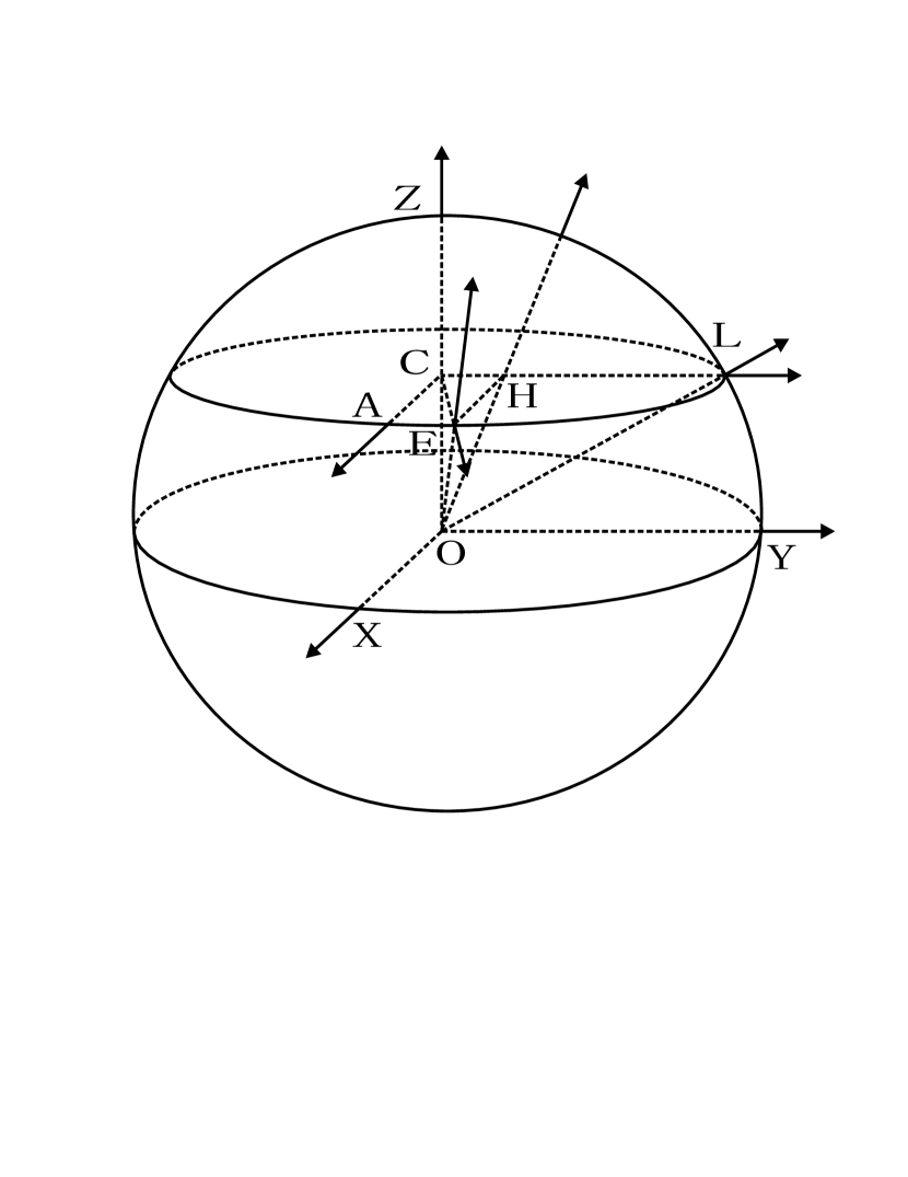
Figure 2: The spatial sketch of the apparent latitude ($\delta$, $\angle{HOY}$), the real latitude ($\theta$, $\angle{LOY}$) and the longitude ($\varphi$, $\angle{ACE}$) of a CME event initiating from the point $E$. $OX$ is the direction of the observer, $OE$ is the direction of CME motion, $CA//OX$, $CL//OY$, and $EH\perp CL$.

The proposed method is based on the assumption of radial motion and uniform longitudinal distribution of CMEs. As shown in Figure 2, the point $E$ indicates the CME source region, $OE$ is the direction of CME motion, $OH$ is $OE$’s projection onto the plane of the sky. Thereupon $\angle{HOY}$, $\angle{LOY}$, and $\angle{ACE}$ are, namely, the apparent latitude $\delta$, the real latitude $\theta$ and the longitude $\varphi$. By a simple deduction ($|CH|=|CE|\sin\varphi=|OC|/\tan\delta$, $|CE|=R_{s}\cos\theta$, $|OC|=R_{s}\sin\theta$) we have

$$\tan\theta=\sin\varphi\tan\delta.$$ (2)

Set the discrete variable $\theta=[0^{\circ},1^{\circ},2^{\circ},\ldots,90^{\circ}]$. For each $\theta$ fixed, we can obtain 91 $\delta$ values by using Equation 2 if given $\varphi=0^{\circ}$, $\varphi=1^{\circ},\cdots,\varphi=90^{\circ}$. We let all $\delta$ equal to the expression $\delta+0.5^{\circ}$ converted to integer type and then we can define a vector $A=[a_{0},a_{1},\ldots,a_{i},\ldots,a_{90}]^{T}$, where $a_{i}$ means the percentage at $\delta=i^{\circ}$ in the obtained 91 $\delta$ values. Some special conditions are dealt with as follows. When $\theta=0^{\circ}$, $A=[1,0,\ldots,0]^{T}$; when $\theta=90^{\circ}$, $A=[0,\ldots,0,1]^{T}$; when $\varphi=0^{\circ}$ and $\theta\neq 0^{\circ}$, $\delta=90^{\circ}$.

Combining 91 vectors $A$ we get a $91\times 91$ matrix

$$M=[A_{0},A_{1},\ldots,A_{j},\ldots,A_{90}],$$ (3)

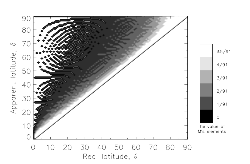
Figure 3: The contour of the transition matrix $M$ defined in section 3. The distributions of the apparent ($S$) and real ($R$) CME latitudes are related by the equation $S=M\times R$. Bright white in the upper left and down right corners indicates the value of zero only for being pleasing to the eye. The bin widths of $\theta$ and $\delta$ are both $1^{\circ}$.

where the subscript $j$ means the case $\theta=j^{\circ}$. Figure 3 shows the contour of matrix $M$. If we use vector $R=[r_{0},r_{1},\ldots,r_{90}]^{T}$ to indicate the real distribution of $\theta$, we have $M\times R=S$ and

$$R=M^{-1}\times S.$$ (4)

4 Results and Discussion

The final results of $R$, also smoothed with a window of $10^{\circ}$, are plotted as 22 thick solid lines in Figure 1. In comparison with $S$, most high-latitude CMEs are substituted with events coming from low latitudes. The reason of this phenomenon is that by projection the CMEs remote from solar limb can be observed at any $\delta>\theta$. For a direct demonstration of the solar cycle variation of $\theta$, we combine all vectors $R$ in time order and give a filled contour plot in Figure 4a. Figure 4b then shows the variation of the actual (not the percentage) CME occurrence rate $\eta=R\times n/t$, where $n$ is the CME number, $t$ is the time length (in $year$), both given in Figure 1.

From Figure 4, we find that most high-latitude CMEs occur during the period from 1999 to the middle of 2001. Gopalswamy et al. (2003) found a general spreading of CME latitudes attaining $60^{\circ}$ by 1999. The northern high-latitude CMEs became nonexist beyond October 2000. However the southern ones continued to occur until the first quarter of 2002. Our time interval of most high-latitude CMEs’ occurrence is approximately consistent with the above Gopalswamy et al.’s. As shown by white dotted lines, we find a poleward motion with a speed of 12.5 $deg/year$ and an equatorward motion with a speed of 25.4 $deg/year$ taking place during years 1999-2001 and during 2000 to the middle of 2001, respectively. For the poleward motion, years 1999 and 2001 are the polarity reversal time at $\theta=60^{\circ}$ and the epoch when the polar regions’ area is of minimum (Song & Wang, 2006). Therefore we suggest this motion come from the collision between the unipolar poleward meridional flows (Song & Wang, 2006) and the polar regions of an opposite polarity. Such collision hastens the formation of polar crown filaments whose eruptions have a close correspondence with CMEs (Gopalswamy et al. 2003). The much lower speed than that of the meridional flows ($>20$ $deg/year$) can be explained by the polar regions blocking the way. The equatorward motion may have the same mechanism because during its interval, we can see that the tilt angle, defined as the maximum extent of the heliospheric current sheet (HCS), also declines sharply with a similar speed (see Figure 8 in Gopalswamy et al. 2003). The high-latitude CMEs constitute 5-10% during the time when the polar magnetic fields reverse sign and 3% of all CMEs during the whole solar cycle.

In the range $\theta\in[45^{\circ},60^{\circ}]$, we only find three prominent peaks located in 2000, near the middle of 2002 and in 2005, respectively, which seem to have a period of 2.5 $years$. By comparing these peak positions with the variation of sunspot number (see the pink solid lines in Figure 4), we find no any close correlations. Therefore this phenomenon is very puzzling indeed. Wang et al. (1989) found many poleward surges of alternating polarities in the active belts. Do they initiate the middle-latitude CMEs? We have no definite answer at present. Such CMEs constitute 6-12% during their main phases and 4% of all CMEs.

93% CMEs occur in the range $\theta<45^{\circ}$. From Figure 4, we find that the highest occurrence probability ($R$) of these low-latitude CMEs is at the minimum and during the declining phase of solar cycle. However the highest occurrence rate ($\eta$) is at the maximum and during the declining phase of solar cycle. As shown by green solid lines, at the minimum and during the rising phase, CMEs’ average latitude has a linear increase. Then at the maximum and during the declining phase, CMEs’ average latitude is in a nearly steady state, which keeps around $15^{\circ}\sim 25^{\circ}$. It is obvious that it does not follow the Spörer sunspot law. This means that there are a large quantity of CMEs originating outside active regions. Zhou et al. (2006) classified CME-associated large-scale structures into four different categories: extended bipolar regions (EBRs), transequatorial magnetic loops, transequatorial filaments and long filaments along the boundaries of EBRs (maybe corresponding to the high-latitude CMEs). The latitudes of former three categories are higher or lower than active regions, which result in a much wider distribution of CME latitudes.

5 Conclusions

Using the proposed method, we have studied the solar cycle variation of real CME latitudes during cycle 23 and found three main features. (1) The latitudinal drift of the high-latitude CMEs ($\theta>60^{\circ}$) was correlated with that of the HCS. (2) The mid-latitude CMEs ($\theta\in[45^{\circ},60^{\circ}]$) occurred primarily in 2000, near the middle of 2002 and in 2005, respectively, forming a prominent three-peak structure. (3) The latitudinal evolution of low-latitude CMEs ($\theta<45^{\circ}$) did not follow the Spörer sunspot law, which suggests that many CMEs originated outside of active regions. We believe that such features can provide hints for understanding the origin of CMEs. At present, Solar Terrestrial Relations Observatory (STEREO), a very nice mission of NASA and launched successfully last October, is observing solar corona in 3-D instead of on the plane of the sky. With it the finding of CME source regions is no longer a difficult thing and then real CME latitude distribution can be better determined.

Figure 1: The distributions of the apparent ($S$, thin solid line) and real ($R$, thick solid line) CME latitudes during 22 time intervals which are smoothed with a window of $10^{\circ}$. The dashed lines around them indicate the unsmoothed variations. In the top right corner of each plot, the time range and the CMEs number have been shown.

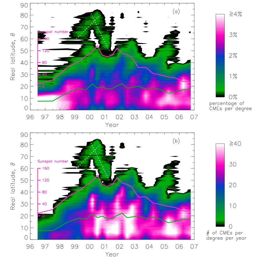
Figure 4: The solar cycle variations of the real CME latitude $\theta$ (a) and the CME occurrence rate $\eta$ (b). The white dotted lines show the poleward and equatorward motions of the high-latitude CMEs. The pink solid line indicates the monthly averaged sunspot number during each period of time. The green solid line indicates the average latitude of CMEs in the range $\theta<45^{\circ}$. Bright white in the upper regions indicates the value of zero.

References

- (1) Gopalswamy, N., Lara, A., Yashiro, S., et al. 2003, International Solar Cycle Studies (ISCS) Symposium, ’Solar Variability as an Input to the Earth’s Environment’, 403
- (2) Gosling, J.T. 1993, JGR, 98, 18937
- (3) Hansen, R., & Hansen, S. 1975, Sol. Phys., 44, 225
- (4) Li, K.J., Schmieder, B., & Li, Q.S. 1998, A&AS, 131, 99
- (5) Oliver, R., & Ballester, J.L. 1994, Sol. Phys., 152, 481
- (6) Skirgiello, M. 2003, GRL, 30, SSC1
- (7) Song, W.B., & Wang, J.X. 2006, ApJ, 643, L69
- (8) St. Cyr, O.C., Howard, R.A., Sheeley, N.R., et al. 2000, JGR, 105, 8169
- (9) Subramanian, P. & Dere, K.P. 2001, ApJ, 561, 372
- (10) Wang, Y.-M., Nash, A.G., & Sheeley, N.R. 1989, Science, 245, 712
- (11) Zhou, G.P., Wang, J.X., & Cao, Z.L. 2003, A&A, 397, 1057
- (12) Zhou, G.P., Wang, J.X., & Zhang, J. 2006, A&A, 445, 1133