Dynamic Boundaries in Asymmetric Exclusion Processes

Abstract

We investigate the dynamics of a one-dimensional asymmetric exclusion process with Langmuir kinetics and a fluctuating wall. At the left boundary, particles are injected onto the lattice; from there, the particles hop to the right. Along the lattice, particles can adsorb or desorb, and the right boundary is defined by a wall particle. The confining wall particle has intrinsic forward and backward hopping, a net leftward drift, and cannot desorb. Performing Monte Carlo simulations and using a moving-frame finite segment approach coupled to mean field theory, we find the parameter regimes in which the wall acquires a steady state position. In other regimes, the wall will either drift to the left and fall off the lattice at the injection site, or drift indefinitely to the right. Our results are discussed in the context of non-equilibrium phases of the system, fluctuating boundary layers, and particle densities in the lab frame versus the frame of the fluctuating wall.

I Introduction

Asymmetric exclusion models with a fixed Schutz and Domany (1993); Derrida et al. (1992, 1993), and typically large number of lattice sites have been the subject of much recent theoretical attention Sandow (1994); Kolomeisky (1998); Chou and Lakatos (2004); Lakatos and Chou (2003); Shaw et al. (2003); Evans et al. (1994); Lahiri and Ramaswamy (1997); Lahiri et al. (2000); Alimohammadi and Naimi (2005); Evans et al. (2003); Parmeggiani et al. (2003, 2004). Biophysical applications and new fundamental understanding of non-equilibrium steady-states (NESS) have motivated many extensions of the simple totally asymmetric exclusion process (TASEP) with open boundaries. These include partially asymmetric models, where particles can hop backward Sandow (1994), exclusion processes with nonuniform hopping rates Kolomeisky (1998); Chou and Lakatos (2004); Lakatos et al. (2006), exclusion among particles of arbitrary size Lakatos and Chou (2003); Shaw et al. (2003); Dong et al. (2007), multispecies exclusion processes Evans et al. (1994); Lahiri and Ramaswamy (1997); Lahiri et al. (2000); Alimohammadi and Naimi (2005), multichannel exclusion processes Pronina and Kolomeisky (2005) and exclusion processes with Langmuir type adsorption and desorption kinetics Evans et al. (2003); Parmeggiani et al. (2003, 2004). All of these studies have considered open, well-defined boundaries, where the length of the lattice is fixed. TASEP models with one open and one closed boundary conditions have also been considered Muller et al. (2005).

However, applications may arise where the length of the system is dynamically varying. The system size may vary because a single particle pushes against a boundary-defining wall. One example is helicase-induced opening of replication forks in DNA processing Betterton and Julicher (2005). Here, the moving replication fork defines a moving boundary of the system. Examples of variable-system size exclusion processes that involve multiple motor particles include mRNA translation in the presence of hairpins in the mRNA, and molecular motors processing on elongating actin filaments. Ribosomes that process along mRNA (in the process of protein synthesis) during translation MacDonald et al. (1968); Chou and Lakatos (2004) often encounter a hairpin and the position at which the hairpin starts represents a wall over which the processing ribosomes cannot pass. The detachment rates of the ribosomes and the tightness of the hairpin may determine if the ribosomes can translate the mRNA through the hairpin sequences. Actin polymerization at the leading edge of filopodia also seems to be mediated by processing molecular motors that may carry actin assembly components Mitchison and Cramer (1996); Soldati (2003). The motors detach, and possibly attach, anywhere along the growing actin filament Klumpp and Lipowsky (2004). The depolymerization of the leading tip may be limited or enhanced by the presence of a motor or other actin associated proteins Dickinson et al. (2004); Klein et al. (2005). Finally, a recent model of a dynamically extending exclusion process without Langmiur kinetics has been recently studied Sugden and Evans (2007). This model has been applied to filamentous hyphae growth in fungi Sugden et al. (2007).

With the above applications in mind, we consider a TASEP with a dynamically varying length. Specifically, we analyze a many-particle asymmetric exclusion process with a fixed open boundary on the left, a fluctuating boundary on the right, and Langmuir kinetics. The particles have a fixed injection site and can adsorb and desorb. A wall with an intrinsic leftward drift (representing e.g., a hairpin which energetically favors spontaneous closing or the barbed end of an actin filament that prefers depolymerization) prevents the passage of particles. The particles advance and provide a pressure against the wall. For certain attachment/detachment and wall hopping rates, the system reaches a NESS in which the statistics of the wall position are stationary. For other values of the kinetic parameters, no time-independent mean wall position exists. The wall will either drift steadily towards the particle injection site and fall off the lattice, or move indefinitely away from the injection site, continuously increasing the size of the system. The specific details of the stochastic process are shown in Figure 1. Particles are injected into the first lattice site with rate $\alpha$ provided it is empty. In the interior of the lattice, each particle moves forward with rate $p$ only if the site ahead of it is unoccupied. Particle attachment and detachment occur with rate $k_{+}$ and $k_{-}$, respectively, throughout the lattice.

Figure 1: A totally asymmetric exclusion process bounded by a fluctuating wall. Particles are injected onto the leftmost site with rate $\alpha$, and move to the right with rate $p$. In the interior, particles detach and adsorb with rates $k_{-}$ and $k_{+}$, respectively where $k_{\pm}\ll p$. The lattice is bounded on the right by a fluctuating wall with intrinsic hopping rates $w_{+}$ and $w_{-}$, where $w_{+}<w_{-}$.

The lattice length is not fixed, and $N$ denotes the position of the particle-confining wall that hops forward with rate $w_{+}$, and backward with rate $w_{-}$ provided there is no particle to its immediate left. The particle occupation at each site, $1\leq i\leq N-1$, left of the wall is represented by the occupation variable $\sigma_{i}\in\{0,1\}$. If $w_{-}\leq w_{+}$, the wall will move indefinitely away from the injection site. In order to prevent the wall from always escaping to infinity, we consider the more interesting case of an intrinsic leftward drift described by $w_{-}>w_{+}$.

The wall position $N$ is not fixed (even at steady state), but rather, is determined by the intrinsic wall hopping rates, and the exclusionary interactions between the wall and the lattice particles. Our analysis is aimed at understanding how the wall dynamics depend on the parameters $\alpha,k_{\pm},w_{\pm},p$. In the next section, we derive relations for the distribution functions of the wall. In steady-state, these relations constrain the particle density at the wall. In Section III, we use mean field theory (MFT) to solve for the density profile, and show that the density profile obtained using mean field theory is inaccurate near the wall. Since quantitative prediction of the wall dynamics will require accurate determination of the particle densities near the wall, in Section IV, we develop a moving-frame finite segment mean field approach to accurately solve for the density profile near the wall. The existence of a steady-state solution and the dependencies of the mean wall position $\langle N\rangle$ on the problem parameters are explored and plotted in Section V.

II Wall dynamics

The net drift of the wall is the difference between its forward and effective backward hopping rates. The effective backward hopping rate depends on both the intrinsic backward hopping rate $w_{-}$, and on the occupancy of the site immediately to the left of the wall since a particle there will block the wall’s backward motion. The wall’s rightward hopping is never impeded. The probability of finding a particle immediately to the wall’s left varies with its position, thus, the wall dynamics are position-dependent. Define $Q_{N}(t)$ as the probability that the wall is at position $N$ at time $t$, and $Q^{\prime}_{N}(t)$ as the joint probability that the wall is at position $N$ at time $t$ and the site just before the wall is empty. The wall dynamics obey

$$\dot{Q}_{N}(t)=w_{-}Q^{\prime}_{N+1}-w_{-}Q^{\prime}_{N}-w_{+}Q_{N}+w_{+}Q_{N-1},$$ (1)

and the moments of the wall position can be formally expressed as

$${\partial\over\partial t}\langle N^{k}\rangle=\sum_{N=0}^{\infty}(w_{-}Q_{N}^{\prime}-w_{+}Q_{N})\sum_{j=0}^{k-1}(-1)^{k-j}{k\choose j}N^{j}.$$ (2)

Although one cannot find $Q_{N}$ or $Q^{\prime}_{N}$ explicitly without solving the full exclusion problem, we can take $k=1$ in (2) to determine the mean wall velocity via

$${\partial\over\partial t}\langle N\rangle=-w_{-}\sum_{N=0}^{\infty}Q^{\prime}_{N}+w_{+}.$$ (3)

If the mean wall position is time-independent, $\sum_{N=0}^{\infty}Q^{\prime}_{N}=w_{+}/w_{-}$, and the expected occupancy of the site immediately preceding the wall is

$$\langle\sigma_{N-1}\rangle=1-\sum_{N=0}^{\infty}Q^{\prime}_{N}=1-\frac{w_{+}}{w_{-}}.$$ (4)

We show in section V.2 that there are some parameter regimes in which (4) cannot be satisfied. For these parameter values, there exists no time-independent mean wall position. However, one can still use (3) to determine the relevant mean wall dynamics. The preceding analysis suggests that it may be more natural to define sites near the wall by their position relative to the wall than by their absolute position on the lattice. To avoid working in both frames of reference, in the next section, we will begin by considering the limit in which the wall hopping rates are small compared to other rates in the problem ($p$, $k_{+}$, and $k_{-}$). In this limit, the wall dynamics are slow compared to the particle dynamics, and we will assume that the wall frame is stationary.

III Mean Field Solution of Density Profile

In the $w_{\pm}/k_{\pm},w_{\pm}/p\rightarrow 0$ limit, we expect the wall to be nearly stationary. Mean field equations can be derived by ensemble-averaging the rate equations for the occupation variables $\sigma_{i}$, and ignoring correlations ($\langle\sigma_{i}\sigma_{j}\rangle\approx\langle\sigma_{i}\rangle\langle\sigma_{j}\rangle$). Upon defining the mean occupation $s_{i}\equiv\langle\sigma_{i}\rangle$, the mean field equations for a fixed ($w_{\pm}=0$) wall system in NESS are

$$\displaystyle{\mbox{d}s_{i}\over\mbox{d}t}=-s_{i}(1-s_{i+1})+s_{i-1}(1-s_{i})-k_{-}s_{i}\qquad$$

$$+k_{+}(1-s_{i})=0,\qquad$$ (5)

$$\displaystyle{\mbox{d}s_{1}\over\mbox{d}t}=\alpha(1-s_{1})-k_{-}s_{1}-s_{1}(1-s_{2})\qquad\,\,\,$$

$$+k_{+}(1-s_{1})=0,\qquad\qquad\,\,$$ (6)

$$\displaystyle{\mbox{d}s_{N-1}\over\mbox{d}t}=-k_{-}s_{N-1}+k_{+}(1-s_{N-1})\qquad\qquad\qquad\,$$

$$\>+s_{N-2}(1-s_{N-1})=0.\qquad\quad$$ (7)

where the adsorption, desorption and injection rates have been normalized by $p$ and time has been rescaled by $p^{-1}$ – hence, $k_{\pm}$, $\alpha$ and $t$ in (5-7) are dimensionless.

However, in order to use condition (4), we need expressions for particle density at sites defined by their distance from the wall. In the fluctuating frame of the wall, we use the notation $\tilde{s}_{j}\equiv s_{N-j}$. Upon rewriting (5-7) in the wall frame, we find

$$\displaystyle\frac{\mbox{d}\tilde{s}_{j}}{\mbox{d}t} = \displaystyle-(1+w_{+})\tilde{s}_{j}(1-\tilde{s}_{j-1})+(1+(1-\tilde{s}_{1})w_{-})\tilde{s}_{j+1}(1-\tilde{s}_{j})-k_{-}\tilde{s}_{j}+k_{+}(1-\tilde{s}_{j})$$

$$\displaystyle\hskip 128.0374pt-w_{-}(1-\tilde{s}_{1})(1-\tilde{s}_{j+1})\tilde{s}_{j}+w_{+}(1-\tilde{s}_{j})\tilde{s}_{j-1}=0,$$ (8)

$$\displaystyle{\mbox{d}\tilde{s}_{N-1}\over\mbox{d}t} = \displaystyle\alpha(1-\tilde{s}_{N-1})-k_{-}\tilde{s}_{N-1}-\tilde{s}_{N-1}(1-\tilde{s}_{N-2})+k_{+}(1-\tilde{s}_{N-1})=0,$$ (9)

$$\displaystyle{\mbox{d}\tilde{s}_{1}\over\mbox{d}t} = \displaystyle-k_{-}\tilde{s}_{1}+k_{+}(1-\tilde{s}_{1})+(1+w_{-})\tilde{s}_{2}(1-\tilde{s}_{1})-\tilde{s}_{1}w_{+}=0.$$ (10)

As expected, (8) and (10) reduce to (5) and (7) in the $w_{\pm}=0$ limit. If the position of the wall were fixed, we could simply use the iteration given by (5), along with boundary conditions (6) and (7) to solve for the density profile $s_{i}$.

Now consider a moving wall problem. Because $\langle N\rangle$ is undetermined, we need three conditions to solve (8). In addition to the two boundary conditions (9) and (10), we require a third condition, $\tilde{s}_{1}=1-w_{+}/w_{-}$, to determine $\langle N\rangle$. This third boundary condition fixes $\tilde{s}_{1}$; $\tilde{s}_{2}$ is set by (10), and we can use (8) to iterate forward in $j$ as many times as required toward the injection site, until (9) is satisfied. The number of iterations required to satisfy (9) determines the mean position, $\langle N\rangle$, of the left boundary, and hence the NESS size reached by the system. Although (8) was derived in the wall frame, the resulting density profile is nearly identical to a stationary frame profile derived from (5) when $s_{i}$ is not varying rapidly with site $i$. See the Appendix for further discussion.

Figure 2: (Color online) A comparison of density profiles derived from Monte-Carlo simulation and MFT. (a) The MFT and MC density profiles for conserved particle TASEP are compared ($\alpha=0.6$, $\beta=0.9$, $N=10,000$). Despite differences between MFT and MC in the boundary layers, the particle density at the ends ($i=1$, $i=10000$) are matched through particle conservation. Insets show the left and right boundary layers in detail. (b) For a TASEP with Langmuir kinetics (with $k_{-}=0.01$, $N=300$, $p=1$, and $k_{+},w_{+},w_{-}=0$), the MFT density profile can be appreciably different from the MC results, especially near the boundaries.

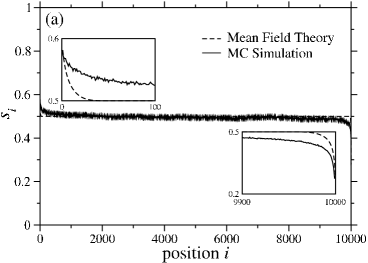
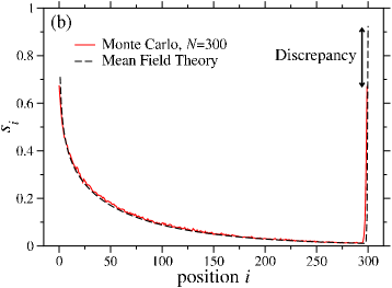
For standard particle-conserving TASEP models, away from boundaries, MFT predicts the particle densities to a very high accuracy Derrida et al. (1992). A conservation law for the particle density can be used to fix the end densities to their exact values so that the MFT also performs well near boundaries Lakatos et al. (2006). In Figure 2a, we plot the density profiles from Monte-Carlo simulations and mean field recursion relations for the simple TASEP ($k_{\pm}=0$) with a fixed number of sites, $N=10000$. Differences in the density profiles are evident in the insets.

Because we include particle adsorption and desorption through Langmuir kinetics, there is no conservation law for the particle density. In this case, the boundary densities are not fixed and we see in Fig. 2b that simple mean field calculations of the boundary density can differ appreciably from the values found from Monte-Carlo simulations. However, MFT still matches simulation results in the bulk where $s_{i}$ varies slowly. In the following section, we use an approach that couples explicit enumeration within a finite segment of sites to the mean field results accurate outside the segment. This finite segment mean field theory (FSMFT) includes particle correlations within a segment of sites adjacent to the wall.

IV Finite Segment Method

We have shown that mean field theory does a poor job of predicting the profile $s_{i\approx N-1}$ near the wall when there is a boundary layer. To more accurately compute the particle density in this region, we will solve the Master equation for a finite segment of $m$ sites preceding the wall. First, we introduce some notation to explain the mechanics of the finite-segment mean field theory (FSMFT). For the binary string $(\sigma_{N-m},...,\sigma_{N-2},\sigma_{N-1})$, corresponding to the occupancy of sites in the finite segment we define the state of the segment as the base ten value of the string. For example, for $m=2$ sites just left of the wall, we have four possible combinations for the occupancies (00), (01), (10), and (11) corresponding to states $i=0,1,2,3$, respectively. If $P_{i}$ is the probability that the finite segment configuration is in state $i$, the Master equation is $\partial_{t}P_{i}=M_{ij}P_{j}$ where $M_{ij}$ is the transition matrix. In the $m=2$ case,

$${\bf M}=\left(\begin{array}[]{cccc}-(1+w_{-})s^{*}-2k_{+}&k_{-}&k_{-}+w_{+}&0\\[13.0pt] k_{+}&-(w_{+}+k_{-}+k_{+})-s^{*}&1+w_{-}(1-s^{*})&k_{-}\\[13.0pt] (1+w_{-})s^{*}+k_{+}&w_{+}&-(w_{+}+w_{-}+1+k_{-}+k_{+})&k_{-}+w_{+}\\[13.0pt] 0&k_{+}+s^{*}&k_{+}+w_{-}s^{*}&-2k_{-}-w_{+}\end{array}\right)$$ (11)

where $s^{*}\equiv\langle\sigma_{N-m-1}\rangle$ is the mean occupancy in the lattice site just to the left of the segment. The mean occupancies in the finite segment can be calculated from ${\bf M}$ in the following way. First, the eigenvector, ${\bf P}^{(0)}$, corresponding to the eigenvalue zero is computed. The vector ${\bf P}^{(0)}$, normalized such that $\sum_{i}^{m}P_{i}^{(0)}=1$ corresponds to the stationary probability distribution, i.e., $\partial_{t}{\bf P}^{(0)}=0$. Let v be a $m\times 2^{m}$ matrix where the columns are the ordered state vectors. The mean densities are then given by $(s_{N-m-1},\ldots,s_{N-2},s_{N-1})^{T}={\bf v}{\bf P}^{(0)}$.

Figure 3: (a) $F(s^{*})$ is plotted with parameter values $k_{+}=0$, $k_{-}=.01$, $w_{+}=0.005$, $w_{-}=0.01$. (b) The finite segment method predicts the boundary layer profile significantly better than mean field theory. Here, the final ten sites of a fixed-wall profile ($N=300$) are plotted. The parameters $k_{-}=0.01$, $k_{+}=0$, and $\alpha=1$ were used.

For every value of $s^{*}$, FSMFT can be used to compute the mean densities $s_{N-m},...,s_{N-2},s_{N-1}$. In particular, it establishes a one-to-one correspondence between $s^{*}$ and $s_{N-1}$:

$$s_{N-1}=F(s^{*};w_{\pm},k_{\pm}).$$ (12)

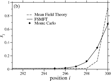
Our calculations indicate that $F(s^{*})$ is always a monotonically increasing function of $s^{*}$, as shown in Figure 3a. Comparing the density profiles near a fixed wall ($w_{+}=w_{-}=0$), Figure 3b shows that using FSMFT (with $m=5$) significantly improves our prediction of the particle density near the wall over that obtained using simple ($m=1$) MFT. To calculate $\langle N\rangle$ for a fluctuating wall ($w_{-}>w_{+}>0$), we first solve for the profile of a segment of sites adjacent to the wall. From (4), when the wall attains a steady-state position, $s_{N-1}=1-w_{+}/w_{-}$. Using (12), we find the value of $s^{*}$ satisfying $1-w_{+}/w_{-}=F(s^{*})$. Defining this particular value of $s^{*}$ as $s^{*}_{eq}$, we then use the recursion relation given by (8) to solve the density profile to the left of the finite segment. Using the values of $s_{N-m}$ and $s^{*}_{eq}\equiv s_{N-m-1}$ from the FSMFT as starting conditions for the recursion equations, we iterate to the left until the left boundary condition (9) is satisfied. In summary, the finite segment mean field theory (FSMFT) is implemented by the following steps:

$\bullet$ For a given $s^{*}$, solve for the normalized eigenvector corresponding to the zero eigenvalue of the $2^{m}\times 2^{m}$ transition matrix $M_{ij}(s^{*})$.

$\bullet$ From the zero eigenvector, express the mean density $s_{N-1}$ at the site nearest the wall as a function of $s^{*}$, giving relation (12).

$\bullet$ For a static wall NESS, set $s_{N-1}=1-w_{+}/w_{-}$ and find $s_{eq}^{*}$ that yields zero net wall drift by using $1-w_{+}/w_{-}=F(s_{eq}^{*};w_{\pm},k_{\pm})$.

$\bullet$ Starting with $\tilde{s}_{m+1}=s_{eq}^{*}$ (and $\tilde{s}_{m}=s_{N-m}$) iterate using the simple mean field equation (8) until equation (9) is satisfied.

$\bullet$ The number of iterations required determines the mean wall position ($\langle N\rangle\approx$ number of iterations $+m+2$) as a function of the rate parameters through the starting value $s_{eq}^{*}$.

We expect the predicted results from a moving-frame FSMFT to be in good agreement with those from MC simulations. This is because in regions where $s$ is slowly varying, the mean field equations describing the density profile in the wall frame and in the lab frame yield nearly identical profiles. This can be seen from the continuum equations, as will be discussed in the Appendix. In these regions, accurate estimates of the mean wall position can also be obtained using the continuum approximations to (8), provided $\langle N\rangle$ is large. When state enumeration of a larger segment is used, more of the correlations within the density boundary layer is taken into account and more accurate results are expected. Provided most of the regions with large gradients in density is captured by the finite segment, the results will be very accurate. The incremental accuracy achieved as larger segments are used has been discussed in a different, but related system Chou and Lakatos (2004). In the subsequent analyses, we use a five-site ($m=5$) FSMFT – generating a $2^{5}\times 2^{5}$ eigenvalue problem in the process – and self-consistently solve for the densities away from the boundary layer. This choice of segment size is sufficient to yield accurate results for all parameters explored.

V Results and Discussion

V.1 Time-Independent Mean Wall Positions

We first consider regimes in which the wall acquires a static mean position in NESS. Using Monte Carlo simulations and FSMFT, we study the dependence of the mean wall position on the injection rate $\alpha$, particle adsorption and desorption rates $k_{\pm}$, and the wall hopping rates $w_{\pm}$. We can use analytic solutions of the bulk continuum equations in order to understand parameter dependencies of our model. Although mean field theory poorly describes our system in the boundary layers where the profile varies rapidly, away from boundary layers, simple MFT is accurate. In these regions, to guide our our analysis, we will use the continuum limit of the mean field equations. We define $\varepsilon\equiv 1/N_{0}$ where $N_{0}$ is a characteristic number of lattice sites (to be derived below) and $x\equiv(i-1)/N_{0}$ as a relative position along the lattice. As shown in the Appendix, the NESS density profile obeys

$$\varepsilon(2s-1)s^{\prime}(x)+k_{+}-(k_{+}+k_{-})s+O(\varepsilon^{2})=0$$ (13)

in both the lab and wall frames of reference. Upon integrating, we obtain the implicit equation

$$\begin{array}[]{l}\displaystyle\frac{(k_{+}-k_{-})\ln|k_{+}-(k_{+}+k_{-})s|-2k_{+}+2(k_{+}+k_{-})s}{(k_{+}+k_{-})^{2}}\\[13.0pt] \hskip 142.26378pt\displaystyle={x\over\varepsilon}+C,\end{array}$$ (14)

where $C$ is a constant of integration. In the continuum description, the entrance site is at position $x=0$, the wall’s position is $L$, and the mean wall position is $\langle L\rangle\equiv\varepsilon\langle N\rangle$. We can use (14) to understand the behavior of the mean wall position $\langle N\rangle$. First, note that the left hand side of (14) scales as $(k_{+}+k_{-})^{-1}$. Since $\varepsilon^{-1}\equiv N_{0}$ scales as $(k_{-}+k_{+})^{-1}$, we define $N_{0}\equiv(k_{+}+k_{-})^{-1}$. For a continuum description to be useful, $N_{0}$ must be large, so $k_{\pm}$ must be small.

Figure 4: (Color online) Simulations were performed with $w_{+}=0.001$, $w_{-}=0.01$, $k_{-}=0.01$, and different values of $\alpha$. In (a), profiles for three simulations are plotted with their mean wall positions aligned. When $\alpha\lesssim 0.5$, $s(0)\approx\alpha$. When $\alpha\gtrsim 0.5$, $s_{B}$ becomes multivalued and there is a boundary layer on the left. Within the boundary layer, a small change in the position results in a large change in the particle density. Thus, in (b), where $\langle N\rangle$ is plotted as a function of $\alpha$, large changes in $\alpha$ result in small changes in $\langle N\rangle$ when $\alpha\gtrsim 0.5$. Also shown is the prediction from (16) with $s_{eq}^{*}=0.026$, determined by FSMFT.

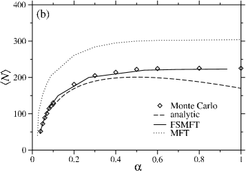
Equation (14) gives an implicit formula for the bulk density, which we denote by $s_{B}(x)$, in terms of the adsorption and desorption rates, $k_{\pm}$ and the integration constant $C$. The injection rate $\alpha$ determines $C$, and along with the wall hopping rates $w_{\pm}$, determines the mean wall position. As shown in the Appendix, the solution near the left boundary varies slowly when $\alpha\lesssim 0.5$. Furthermore, if $k_{-}\ll\alpha$, we can approximate $s_{1}\approx s_{2}$ in (6) to conclude that $s(0)\approx\alpha$. This simplified condition can be used to determine $C$ in (14).

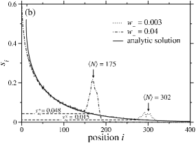
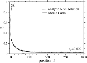
When $\alpha\gtrsim 0.5$, a boundary layer arises on the left (this can be seen in Fig. 4a). In this regime, $s(0)$ can no longer be approximated as $\alpha$, and $s_{B}(x)$ becomes invalid near the injection site. While $s_{B}(x)$ is still a good approximation to the density profile outside the boundary layer (where $s\lesssim 0.5$), there is no straightforward, analytic way to calculate $C$ when $\alpha\gtrsim 0.5$. In Fig. 4a, when $\alpha=1$, $C$ is used as a single fitting parameter and is determined empirically such that in the bulk, $s_{B}(x)$ approximates the density profile obtained using MC simulations. The mean wall position, $\langle L\rangle$, is found through the relation $s_{B}(\langle L\rangle-(m+1))=s^{*}_{eq}$ where $s^{*}_{eq}$ is found using an $m-$site FSMFT and is the value of $s^{*}$ that puts no net drift on the wall.

Figure 4a shows results from MC simulations, shifted so that the mean wall positions are aligned at $\langle N\rangle=225$, which is the mean wall position when $\alpha=1$. While the density profile has a sharp boundary layer at the wall in the wall frame, in the lab frame, the boundary layer is smeared out due to wall fluctuations. This results in the broad peaks centered on the mean wall position seen in Figure 4a. The outer solution $s_{B}(i/N_{0})$ with $N_{0}=(k_{+}+k_{-})^{-1}$ is shown by the dotted curve. The close agreement between the MC data and $s_{B}(x)$ suggests that dropping the $O(\varepsilon^{2})$ term in (13) to obtain $s_{B}(x)$ produces an excellent approximation to the mean particle density, provided $\alpha\lesssim 0.5$. Note that $\alpha$, through $C$, simply shifts $s_{B}(x)$ to the left or right; thus, when we vary only $\alpha$ and plot the resulting density with the mean wall positions aligned (as they are in 4a), the profiles collapse onto the same curve.

We can also use (14) to predict the mean wall position as a function of the injection rate $\alpha$ when $\alpha$ is not too large. For simplicity, consider $k_{+}=0$ – the analysis for $k_{+}\neq 0$ is analogous. Using the simplified condition $s(0)=\alpha$ in (14), we have

$$C={2\alpha-\ln(\alpha k_{-})\over k_{-}}.$$ (15)

Now, using the relation $s^{*}_{eq}=s_{B}(\langle L\rangle-\varepsilon(m+1))$ and (15), (14) becomes

$$\langle N\rangle=\frac{1}{k_{-}}\ln\left(\frac{\alpha}{e^{2\alpha}}\frac{e^{2s^{*}_{eq}}}{s^{*}_{eq}}\right)+m+1.$$ (16)

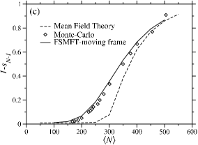
The dependence of $\langle N\rangle$ on $\alpha$ is shown in Figure 4b, predicted using four different methods. Simple MFT ($m=1$, dotted curve) performs poorly relative to MC simulations (open diamonds). The results from FSMFT with $m=5$ (solid curve) agree very well with the MC data for all values of $\alpha$. The solution of (16) (dashed curve) performs reasonably well provided $\alpha$ is not too large. When $\alpha\gtrsim 0.5$, $s(0)=\alpha$ is a poor approximation to (6) and the resulting prediction of $\langle N\rangle$ suffers. In fact, the slope $s_{B}^{\prime}$ diverges when $s_{B}=0.5$, which can be seen from (13). When $\alpha\gtrsim 0.5$, there is a boundary layer on the left with width $O(\sqrt{\varepsilon})$ (cf. Appendix). As a result, increases in $\alpha$ above $0.5$ will increase the height of the boundary layer, but will not significantly change the mean wall position, and $\langle N\rangle$ becomes insensitive to changes in $\alpha$ .

Figure 5: Boundary effects near the wall determine wall position. In (a), $s^{*}_{eq}$ is determined empirically from MC simulations captured in the wall frame and numerically using the finite segment method. In (b), MC simulations are plotted in the lab frame. In (c), the occupancy of the last site in the wall frame $s_{N-1}=1-w_{+}/w_{-}$ is plotted as a function of the mean wall position $\langle N\rangle$. The parameters $\alpha=1$, $k_{-}=0.01$, $k_{+}=0$, and $w_{+}=0.001$ were used.

We now discuss how changes in the wall hopping rates can affect the wall position. In Fig. 5a, for a fixed value of $w_{+}$, one sees that an increase in $w_{-}$ increases the value of $s^{*}_{eq}$. Our FSMFT predicts that given values of $w_{+}$ and $w_{-}$, $s^{*}_{eq}$ must satisfy $1-w_{+}/w_{-}=F(s^{*}_{eq};w_{\pm})$. For small values of $w_{\pm}$, $F(s_{eq}^{+},w_{\pm})\approx F(s_{eq}^{*},0)\approx 1-w_{+}/w_{-}$, suggesting that $s^{*}_{eq}$ depends primarily on the ratio $w_{+}/w_{-}$, with only a weak dependence on the individual wall hopping rates. Since $F$ is a monotonically increasing function, $s^{*}_{eq}$ increases with $w_{-}/w_{+}$.

A change in $s_{eq}^{*}$ induces a change in the mean wall position, shown in Fig. 5b. Again, this is consistent with our theory since $\langle L\rangle$ must satisfy $s_{B}(\langle L\rangle-\varepsilon(m+1))=s_{eq}^{*}$. In the special case $\alpha\lesssim 0.5$, one can use (16) to predict $\langle N\rangle$ directly, given $s^{*}_{eq}$. When $\alpha\gtrsim 0.5$, one either has to solve the full set of discrete MFT equations (8) and (9) – or the equivalent continuum equations (27) and (28) – coupled to a finite segment, to obtain $\langle N\rangle$. Our results from solving the discrete equations are shown in Fig. 5(c). Using simple MFT ($m=1$) without a larger finite segment generally results in poor predictions for $\langle N\rangle$.

A more complete understanding of the wall dynamics can be garnered by analyzing the wall fluctuations. For simplicity, we consider the continuum description in which the wall’s motion can be approximately described by a diffusion constant $D=\varepsilon^{2}w_{+}$ and a position-dependent drift, $V(L)$. If one assumes that the wall fluctuates within a harmonic “potential,” this drift takes the form $V(L)=-a(L-\langle L\rangle)$, where $a\equiv-(\mbox{d}V/\mbox{d}L)|_{\langle L\rangle}$. This approximation effectively closes (1) by expressing the effects of conditional probability, $Q_{N}^{\prime}$, in terms of a drift. For $L\approx\langle L\rangle$, the probability density of the wall’s position, $Q(L)$ (the continuum analog of $Q_{N}$), can be approximately found from the solution of

$$\frac{\partial Q(L,t)}{\partial t}=a{\partial\over\partial L}\left[(L-\langle L\rangle)Q(L)\right]+D\frac{\partial^{2}Q}{\partial L^{2}}.$$ (17)

Upon imposing the normalization $\int_{-\infty}^{\infty}Q(L)dL=1$, we find the steady-state solution to (17):

$$Q(L)=\sqrt{\frac{a}{2D\pi}}e^{-\frac{a(L-\langle L\rangle)^{2}}{2D}},$$ (18)

where $a$ is given by

$$a\equiv-\frac{dV}{dL}\bigg{|}_{\langle L\rangle}=-\frac{\partial V}{\partial F}\frac{\partial F}{\partial s^{*}}s_{B}^{\prime}(\langle L\rangle-\varepsilon(m+1)).$$ (19)

The drift velocity $V(L)$ can be inferred from $\varepsilon(w_{+}-w_{-}(1-s_{N-1}))$ and (12), which relates the mean occupancies at positions $L$ and $L-\varepsilon(m+1)$,

$$V(L)=\varepsilon\left[w_{+}-w_{-}+w_{-}F(s^{*}(L-\varepsilon(m+1)))\right].$$ (20)

By defining the drift $V(L)$ using the steady-state relation $F$, we have implicitly made an adiabatic approximation where the particles have reached a NESS for any wall position $L$.

We can also estimate the variance of the wall position by using $\Sigma^{2}\approx D/a$, and (19) for $a$. Upon differentiating $V(L)=\varepsilon(w_{+}-w_{-}[1-F(s_{B}^{\prime}(L-\varepsilon(m+1)])$, we find $(\partial V/\partial F)=\varepsilon w_{-}$. We can estimate $(\partial F/\partial s^{*})|_{s^{*}_{eq}}$ using the finite segment method, and we know $s_{B}^{\prime}(\langle L\rangle-\varepsilon(m+1))$ exactly from (13). Assuming that $\langle L^{2}\rangle\approx\int_{-\infty}^{\infty}dLL^{2}Q(L)$, we expect the variance of the wall position to be approximately

$$\Sigma^{2}=\langle L^{2}\rangle-\langle L\rangle^{2}=\frac{D}{\varepsilon w_{-}F^{\prime}(s^{*}_{eq})s_{B}^{\prime}(\langle L\rangle-\varepsilon(m+1))}$$ (21)

In Figure 6, we plot an example distribution $Q(L)$ found using both Monte Carlo simulations and from (18).

Figure 6: Probability density of the wall position, $Q(L)$, is plotted as a function of the deviation from the mean wall position $\langle L\rangle$. The parameters $\alpha=1$, $w_{+}=0.005$, $w_{-}=0.01$, $k_{-}=0.01$, and $k_{+}=0$ yield $\langle L\rangle\approx 350$. The distribution predicted from (18) is a close approximation to that derived from MC simulations.

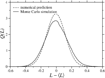
We have aligned the distributions such that their maxima coincide. Using (21), the standard deviation $\Sigma\approx 0.1215$, in good agreement with the standard deviation found from MC simulations $\Sigma\approx 0.143$. Since $\Sigma/\langle L\rangle\sim 0.14/3.5\ll 1$, the wall is fairly stable and not likely to fall off the injection end of the lattice except on exponentially long time scales.

V.2 Time-dependent mean wall positions

In the previous section, we explored the dependence of the statistically stationary mean wall position on the model parameters. However, a stable mean wall position may not always exist. In this section, we use a FSMFT to determine the stability of the wall and the conditions under which a permanent net wall drift might arise.

The motion of the wall can be understood completely in terms of the outer solution $s_{B}(x)$ – given by inverting (14) – and the particle density inside finite segment. First, we consider some important properties of $s_{B}(x)$. Equation (14) admits two branches to the bulk solution, $s_{B}(x)$, because the argument of $\ln[|\quad|]$ can either be positive or negative. The argument approaches zero as $s$ approaches $s_{\Gamma}\equiv k_{+}/(k_{+}+k_{-})$, the density arising from Langmuir kinetics alone. When we invert $x(s_{B})$ to find $s_{B}(x)$, we see that for increasing $x$, one branch of the density profile $s_{B}(x)$ approaches $s_{\Gamma}$ asymptotically from below, and a second branch approaches $s_{\Gamma}$ asymptotically from above. A representative $s_{B}(x)$ is plotted in Figure 7. Notice that $s^{\prime}(x)>0$ in the lower branch, and $s^{\prime}(x)<0$ in the upper branch .

Figure 7: Four possibilities for the wall motion. Arrows indicate the mean wall motion if it is at position $i$. (a) the wall could have no net drift and a stable fixed mean position, with small perturbations to the wall position decaying over time, (b) the wall could have no net drift, but an unstable fixed mean position, with small perturbations to its position causing it to drift indefinitely to the left or right, (c) the wall could drift indefinitely to the left and (d) the wall could drift indefinitely to the right. The outer solution $s_{B}(x)$ is shown by the dotted curves.

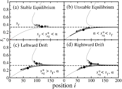
If $\alpha>s_{\Gamma}$, the steady state density profile will lie on the upper branch and the bulk density will have values satisfying $s_{\Gamma}<s_{B}(x)<\alpha$. If the injection rate $\alpha<s_{\Gamma}$, the steady state density profile will lie on the lower branch and the bulk density will attain values $\alpha<s_{B}(x)<s_{\Gamma}$.

We are now ready to derive conditions for the existence of a fixed mean wall position and stability criteria. In the adiabatic approximation (20), $m$ is the number of sites in the finite segment and $\varepsilon=1/N_{0}$. This equation expresses the velocity of the wall at position $\varepsilon N=L$ in terms of a particle density at position $(N-m-1)\varepsilon$. Since $s^{*}_{eq}$ is the value of $s^{*}$ that puts no net drift on the wall, i.e., $w_{+}-w_{-}(1-F(s^{*}_{eq}))=0$, we can expand $V(L)$ from (20) in a Taylor Series about $s^{*}_{eq}$ to find

$$V(L)\approx\varepsilon w_{-}F^{\prime}(s^{*}_{eq})(s^{*}(L-\varepsilon(m+1))-s^{*}_{eq}).$$ (22)

Because $F$ is a monotonically increasing function and $w_{-}>0$, the wall drifts to the right if $s^{*}(L-\varepsilon(m+1))>s^{*}_{eq}$, to the left if $s^{*}(L-\varepsilon(m+1))<s^{*}_{eq}$ and has a fixed mean position if $s^{*}(L-\varepsilon(m+1))=s^{*}_{eq}$. If we now assume that $m$ is sufficiently large so that the point $L-\varepsilon(m+1)$ lies outside of the boundary layer, then $s^{*}(L-\varepsilon(m+1))$ can be well approximated by the outer solution given by $s_{B}(x)$, i.e. $s_{B}(L-\varepsilon(m+1))\approx s^{*}(L-\varepsilon(m+1))$. Furthermore, we know that $s_{B}(x)$ satisfies $\alpha\leq s_{B}\leq s_{\Gamma}$ on the lower branch and $s_{\Gamma}\leq s_{B}\leq\alpha$ on the upper one. Therefore, we conclude that if $s^{*}_{eq}\notin[\alpha,s_{\Gamma}]$, the wall can never have a fixed mean position. In particular, for all $t$

$$\begin{array}[]{rl}V(L(t))&>0\quad\mbox{if}\quad s^{*}_{eq}<\alpha,s_{\Gamma},\\ &<0\quad\mbox{if}\quad s^{*}_{eq}>\alpha,s_{\Gamma},\end{array}$$

corresponding to an indefinite rightward and leftward drift, respectively (cf. Fig. 7c and d). If a fixed mean position does exist, we can understand its stability by considering the sign of $dV/dL$. If this quantity is negative (positive), the position is stable (unstable). These possibilities are summarized in Figure 7. By differentiating (22), we have

$${\mbox{d}V\over\mbox{d}L}\approx\varepsilon w_{-}F^{\prime}(s^{*}_{eq})s_{B}^{\prime}(L-\varepsilon(m+1)).$$ (23)

Hence, if a mean wall position exists at $L$, a necessary and sufficient condition for its stability is

$$s_{B}^{\prime}(L-\varepsilon(m+1))<0.$$ (24)

In particular, when there is no adsorption ($k_{+}=0$), the bulk solution $s_{B}(x)$ decreases monotonically from the injection site and any mean wall position $\langle L\rangle$ induced by the kinetics will be deterministically stable.

Figure 8: In (a), we plot the density profile near the wall from FSMFT and from MC simulations. We find that $s_{N-1}$ is less than $0.9=1-w_{+}/w_{-}$, the value required for the wall to have zero drift. In (b), the position of the wall $N(t)$ found from MC simulations is plotted with the expected $N(t)$ calculated using FSMFT. Parameter values were $\alpha=0.01$, $w_{+}=0.001$, $w_{-}=0.01$, $k_{+}=0.0001$, $k_{-}=0.01$.

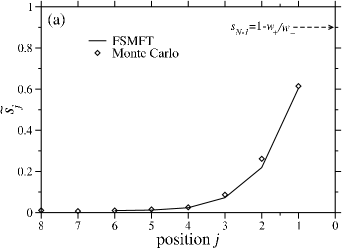
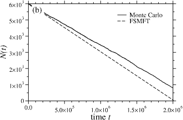
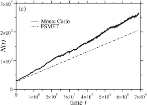
Figures 8 and 9 compare the result (20) with simulation data. Figure 8 shows the results of a MC simulation in which the wall particle has a mean leftward drift. In Fig. 8a, the density profile in the wall frame found from MC simulation and that predicted using FSMFT are shown. Far from the injection site $s_{B}$ asymptotes to $s_{\Gamma}$. Thus, when the wall starts at a position $L_{0}\gg 1$, we assume $s^{*}(L-\varepsilon(m+1))=s_{\Gamma}$ and the wall’s velocity $V$ is independent of its position $L$. Since $s_{N-1}<1-\frac{w_{+}}{w_{-}}$, we expect, from (20), that the net drift on the wall will be negative. In Fig. 8b, we compare $N(t)=L(t)/\varepsilon$ found from MC simulations with that calculated assuming $L(t)=L_{0}+Vt$ where $V$ is calculated using (20) in the large $L$ limit. Similarly, Fig. 9a shows a density profile from MC simulation in the case where the wall acquires a mean rightward drift. In Fig. 9b both MC simulations and FSMFT show that in the wall frame, the occupancy of the site adjacent to the wall is greater than $1-\frac{w_{+}}{w_{-}}$, and we expect a mean rightward drift. In Fig. 9c, we see that this is the case, and the predicted time course $N(t)=L(t)/\varepsilon$ is compared with $N(t)$ found using MC simulations.

In contrast to the case of a static mean wall position, when the wall has a position-independent velocity, $V$, the diffusion constant $D$ of the wall is given by $D=\varepsilon^{2}(w_{+}-w_{-}+w_{-}F(s_{\Gamma}))/2$. The probability density $Q(L,t)$ describing wall position then follows

$$\frac{\partial Q}{\partial t}=D\frac{\partial^{2}Q}{\partial L^{2}}-V\frac{\partial Q}{\partial L},$$ (25)

the solution of which is

$$Q(L,t)=\frac{1}{2\sqrt{\pi Dt}}e^{-\frac{(L-Vt-L_{0})^{2}}{4Dt}}.$$ (26)

We now discuss our results in the context of the phase transitions Evans et al. (2003); Parmeggiani et al. (2004); Popkov et al. (2003) of the interior density. When Langmuir kinetics is coupled to a fixed domain TASEP with open boundaries, qualitative properties of $s(x)$ can change abruptly when adsorption/desorption and injection/ejection rates vary. For example, an interior boundary layer separating regions of low and high density can suddenly disappear, replaced with a single region of high density as the injection rate $\alpha$ is increased.

Our moving wall TASEP system coupled with Langmuir kinetics does not support the phase structure seen in Evans et al. (2003); Parmeggiani et al. (2004); Popkov et al. (2003). Because we limit ourselves to $k_{+}<k_{-}$, we can see from (13) that when $s_{B}(x)>0.5$, (corresponding with a high density region), $s_{B}^{\prime}(x)>0$. From (24), the wall cannot have a stable equilibrium position within the high density region, and we do not find time-independent density profiles with low to high density interior shocks (a low-high shock), as is observed in Evans et al. (2003); Parmeggiani et al. (2004). In fact, references Parmeggiani et al. (2003); Popkov et al. (2003) show that high-low shocks are never stationary in an exclusion process with Langmuir kinetics. Therefore, interior shocks are never stable in our model system. In our problem, the presence of a wall that responds to particle dynamics relaxes any shocks in density that may otherwise occur in the interior, forcing them to the left or right boundaries.

Figure 9: When $s_{\Gamma}>s^{*}_{eq}$ and $\alpha>s^{*}_{eq}$, the wall escapes. In (a), far from the injection site, the particle density approaches $s_{\Gamma}=0.029$ as predicted by analytic theory. In (b), we use FSMFT and MC to find $s_{N-1}>0.9=1-w_{+}/w_{-}$, the value for which the wall’s drift would be zero. In (c), we show $N(t)$ to compare the escape velocity calculated from finite segment analysis to the escape velocity found in simulations. Although the value of $s_{N-1}$ found by FSMFT differs from that found in MC simulations by only $0.4\%$, the calulated velocities differ by $17\%$. Parameter values were $\alpha=0.3$, $w_{+}=0.001$, $w_{-}=0.01$, $k_{+}=0.0003$, and $k_{-}=0.01$.

VI Summary and Conclusions

Our model of an asymmetric exclusion process with Langmuir kinetics and a movable right boundary, and the corresponding results provide a guide to understanding biophysical processes in which many processing molecular motors push against a load. The detachment and attachment rate of the motors, as well as the injection rate at the entry site, determine the load the motors can support. If a static load particle position is reached, we see that the mean wall distance from the injection site saturates upon increasing injection rate $\alpha$ past about $0.5$. The analyses can be used to predict whether biological processes such as ribosome movement and filopodia/filament extension continues or reaches a static configuration.

Within our model, we found four parameter regimes. In the first regime, $(s_{\Gamma}<s_{eq}^{*}<\alpha)$, the wall attains a stable equilibrium position for the wall. In the second regime, $(\alpha<s_{eq}^{*}<s_{\Gamma})$, there is an equilibrium, but unstable mean wall position. In the third and fourth regimes, $(s_{eq}^{*}\notin[\alpha,s_{\Gamma}])$, the wall will always feel a net drift to the to the right and left, respectively. In the latter case, the wall will fall off the lattice in a time scaling linearly with the starting position. When there is a stable equilibrium wall position, we can find the mean wall position $\langle N\rangle$ as a function of the particle injection rate $\alpha$, the adsorption and desorption rates $k_{\pm}$, and the intrinsic hopping rates of the wall $w_{\pm}$. Determination of $\langle N\rangle$ requires accurate evaluation of the particle density near the wall. Using a hybrid finite segment/mean field approach in the reference frame of the fluctuating wall, we accurately determine the particle density near the wall, and use this to determine the wall’s steady-state position.

When there is no steady state wall position, the finite segment mean field approach allows us to estimate the steady state velocity of the wall far from the injection site. In our analysis, we assumed that the particle density has reached steady state, thus ignoring the initial particle density profile and wall position. Even in regimes where we expect an equilibrium wall position at steady state, if the wall is initially near the injection site, and the particle density is initially very low, we would expect the wall to fall off the lattice before reaching its equilibrium position. The times to falling off the lattice may be treated with extensions of large deviation theory as suggested by Fig. 6 Derrida et al. (2003). A number of interesting extensions of the free boundary problem arise. For example, we expect for certain parameter regimes that slow bottleneck sites Chou and Lakatos (2004) can attract the fluctuating wall. These features and other novel applications to biophysical systems deserve investigation.

This material is based upon work supported under a National Science Foundation Graduate Research Fellowship. The authors also acknowledge support from the NSF through grant DMS-0349195, and the NIH through grant K25 AI41935.

VII Appendix

We can take the continuum limit of (5) by defining $x=(i-1)\varepsilon$ where $\varepsilon$ is the lattice spacing. We find,

$${\partial s(x,t)\over\partial t}=\varepsilon s^{\prime}(2s-1)+{\varepsilon^{2}\over 2}s^{\prime\prime}-k_{-}s+k_{+}(1-s)=0.$$ (27)

The left hand boundary condition, (6) becomes

$$\begin{array}[]{l}\displaystyle{\partial s(0,t)\over\partial t}=\alpha(1-s(0))-k_{-}s(0)+k_{+}(1-s(0))-s(0)(1-s(\varepsilon))=0.\end{array}$$ (28)

When significant changes in the solution near $x=0$ vary over a length scale that is $>O(\varepsilon)$, this equation is well approximated by

$$\begin{array}[]{l}\displaystyle{\partial s(0,t)\over\partial t}=\alpha(1-s(0))-k_{-}s(0)+k_{+}(1-s(0))-s(0)(1-s(0)-\varepsilon s^{\prime}(0))=0.\end{array}$$ (29)

The right hand boundary condition analogous to (10), becomes

$$\begin{array}[]{l}\displaystyle{\partial s(L,t)\over\partial t}=-k_{-}s(L)+k_{+}(1-s(L))+s(L-\varepsilon)(1-s(L))+w_{-}s(L-\varepsilon)(1-s(L))-w_{+}s(L)=0.\end{array}$$ (30)

Again, when significant changes in the solution near $x=L$ vary over a length scale that is $>O(\varepsilon)$, this equation is well approximated by

$${\partial s(L,t)\over\partial t}=-k_{-}s(L)+k_{+}(1-s(L))+(s(L)-\varepsilon s^{\prime}(L))(1-s(L))+w_{-}(s(L)-\varepsilon s^{\prime}(L)))(1-s(L))-w_{+}s(L)=0,$$ (31)

at the free boundary $L(t)$, where $s(L)$ defines the particle density at the position just to the left of the wall. In the wall frame, the continuum limit of equation (8) is

$$\begin{array}[]{l}\displaystyle{\partial s(x,t)\over\partial t}=\varepsilon[w_{+}-(1+w_{-}(1-s_{N-1}))]s^{\prime}(1-2s)+{\varepsilon^{2}\over 2}[1+w_{+}+w_{-}(1-s_{N-1})]s^{\prime\prime}-k_{-}s+k_{+}(1-s).\end{array}$$ (32)

In the wall frame, an interior particle shifts to the right when it either hops to the right, which it does with a (normalized) rate of unity, or when the wall hops to the left, which it does with rate $w_{-}(1-s_{N-1})=w_{+}$ in steady state. Similarly, a particle shifts to the left when it hops to the left or when the wall hops to the right, which it does with rate $w_{+}$. In the bulk, where $s^{\prime}(x)=O(1)$, the diffusive term is small and can be neglected. The only term we retain that depends on hopping rates is $(w_{+}-1-w_{+})(1-2s)s^{\prime}$, which is equal to the value of the corresponding term in the lab frame, $-(1-2s)s^{\prime}$. The bulk density is described in both frames by

$$\varepsilon s^{\prime}(1-2s)+k_{-}s-k_{+}(1-s)=0.$$ (33)

In our problem, the second order term in (27) becomes important in the right hand boundary layer, and in the left hand boundary layer when there is one. On the left, when $s\approx 0.5$, one cannot assume that $s$ varies slowly. Making the change of variables $x=\xi X$ ($\xi\ll 1$), equation (27) becomes

$$\frac{\varepsilon}{\xi}s^{\prime}(2s-1)+\frac{\varepsilon^{2}}{2\xi^{2}}s^{\prime\prime}-k_{-}s+k_{+}(1-s)=0;$$ (34)

furthermore, we know that $\varepsilon$ is necessarily on the order $(k_{-}+k_{+})$. Since the first order term becomes very small as $s\rightarrow 0.5$, the second order term must match either the adsorption or desorption term. In this case, the second order term will be balanced when $\xi\sim\sqrt{\varepsilon}$. Therefore, we expect a boundary layer of width $O(\sqrt{\varepsilon})$ to arise near the injection site if $\alpha>0.5$, $s_{\Gamma}<0.5$ or if $\alpha<0.5$ and $s_{\Gamma}>0.5$.

While the boundary layer on the left can be captured using a second order continuum equation, the boundary layer on the right cannot. In equation (27), we kept terms only up to order $\varepsilon^{2}$ in our expansion $s(x+\varepsilon)$ = $s(x)+\varepsilon s^{\prime}(x)+\frac{\varepsilon^{2}}{2}s^{\prime\prime}(x)+\frac{\varepsilon^{3}}{6}s^{(3)}(x)+...$. The boundary layer on the right hand side arises to join the outer solution with the boundary condition $s(L)=1-w_{+}/w_{-}$. Making the substitution $X=x/\xi$, and matching first and second order terms in (34), we find that $\xi=O(\varepsilon)$. In the boundary layer on the left, $s\approx 0.5$, and we assume that the term $\varepsilon(2s-1)s^{\prime}$ is relatively small. When we match the second order term, $\varepsilon s^{\prime\prime}/2$, with the adsorption and desorption terms, $k_{+}(1-s)$ and $k_{-}s$, we find that $\xi\sim\sqrt{\varepsilon}$. However, on the right, we cannot assume that $s\approx 0.5$. We therefore assume that the leading terms are $\varepsilon(2s-1)s^{\prime}$ and $\varepsilon s^{\prime\prime}/2$, which leads us to conclude that the wall-hugging boundary layer has width of $O(\varepsilon)$. In this case, all terms $\varepsilon^{n}s^{(n)}(X)/n!$ in the Taylor expansion of (30) are $O(1)$, and continuum theory breaks down.

References

- Schutz and Domany (1993) G. Schutz and E. Domany, J. Stat. Phys. 72, 277 (1993).
- Derrida et al. (1992) B. Derrida, E. Domany, and D. Mukamel, J. Stat. Phys. 69, 997 (1992).
- Derrida et al. (1993) B. Derrida, S. A. Janowsky, J. L. Lebowitz, and E. R. Speer, J. Stat. Phys. 73, 813 (1993).
- Sandow (1994) S. Sandow, Phys. Rev. E 50, 2660 (1994).
- Kolomeisky (1998) A. B. Kolomeisky, J. Phys. A: Math. Gen 31, 1153 (1998).
- Chou and Lakatos (2004) T. Chou and G. Lakatos, Phys. Rev. Lett. 93, 198101 (2004).
- Lakatos and Chou (2003) G. Lakatos and T. Chou, J. Phys. A: Math. Gen. 36, 2027 (2003).
- Shaw et al. (2003) L. B. Shaw, R. K. P. Zia, and K. H. Lee, Phys. Rev. E 68, 021910 (2003).
- Evans et al. (1994) M. R. Evans, D. P. Foster, C. Godreche, and D. Mukamel, J. Stat. Phys. 80, 69 (1994).
- Lahiri and Ramaswamy (1997) R. Lahiri and S. Ramaswamy, Phys. Rev. Lett. 79, 1150 (1997).
- Lahiri et al. (2000) R. Lahiri, M. Barma, and S. Ramaswamy, Phys. Rev. E 61, 1648 (2000).
- Alimohammadi and Naimi (2005) M. Alimohammadi and Y. Naimi, J. Math. Phys. 46, 053306 (2005).
- Evans et al. (2003) M. R. Evans, R. Juhász, and L. Santen, Phys. Rev. E 68, 026117 (2003).
- Parmeggiani et al. (2003) A. Parmeggiani, T. Franosch, and E. Frey, Phys. Rev. Lett. 90, 086601 (2003).
- Parmeggiani et al. (2004) A. Parmeggiani, T. Franosch, and E. Frey, Phys. Rev. E 70, 046101 (2004).
- Lakatos et al. (2006) G. Lakatos, J. O’Brien, and T. Chou, J. Phys. A: Math. Gen. 39, 2253 (2006).
- Dong et al. (2007) J. J. Dong, B. Schmittmann, and R. K. P. Zia, In Press: J. Stat. Phys. (2007).
- Pronina and Kolomeisky (2005) E. Pronina and A. B. Kolomeisky, J. Stat. Mech. p. P07010 (2005).
- Muller et al. (2005) M. J. I. Muller, S. Klumpp, and R. Lipowsky, J. Phys.: Condens. Matter 17, S3839 (2005).
- Betterton and Julicher (2005) M. D. Betterton and F. Julicher, Phys. Rev. E 71, 011904 (2005).
- MacDonald et al. (1968) C. T. MacDonald, J. H. Gibbs, and A. C. Pipkin, Biopolymers 6, 1 (1968).
- Mitchison and Cramer (1996) T. J. Mitchison and L. P. Cramer, Cell 84, 371 (1996).
- Soldati (2003) T. Soldati, Traffic 4, 358 (2003).
- Klumpp and Lipowsky (2004) S. Klumpp and R. Lipowsky, J. Stat. Phys. 113, 233 (2004).
- Dickinson et al. (2004) R. B. Dickinson, L. Caro, and D. L. Purich, Biophys. J. 87, 2838 (2004).
- Klein et al. (2005) G. Klein, K. Kruse, G. Cuniberti, and F. Jülicher, Phys. Rev. Lett. 94, 108102 (2005).
- Sugden and Evans (2007) K. E. P. Sugden and M. R. Evans, arXiv:0707.4504 (2007).
- Sugden et al. (2007) K. E. P. Sugden, M. R. Evans, W. C. K. Poon, and N. D. Read, Phys. Rev. E 75, 031909 (2007).
- Popkov et al. (2003) V. Popkov, A. Rákos, R. D. Willmann, A. B. Kolomeisky, and G. M. Schutz, Phys. Rev. E 67, 066117 (2003).
- Derrida et al. (2003) B. Derrida, J. L. Lebowitz, and E. R. Speer, J. Stat. Phys. 110, 775 (2003).