Nucleon Spin Structure with hadronic collisions at COMPASS

Abstract

In order to illustrate the capabilities of COMPASS using a hadronic beam, I review some of the azimuthal asymmetries in hadronic collisions, that allow for the extraction of transversity, Sivers and Boer-Mulders functions, necessary to explore the partonic spin structure of the nucleon. I also report on some Monte Carlo simulations of such asymmetries for the production of Drell-Yan lepton pairs from the collision of high-energy pions on a transversely polarized proton target.

I Introduction

The recent measurement of Single-Spin Asymmetries (SSA) in semi-inclusive $lp^{\uparrow}\to l^{\prime}\pi X$ Deep-Inelastic Scattering (SIDIS) on transversely polarized hadronic targets Airapetian et al. (2005); Diefenthaler (2005); Avakian et al. (2005); Alexakhin et al. (2005), has renewed the interest in the problem of describing the spin structure of hadrons within Quantum Chromo-Dynamics (QCD) Radici and van der Steenhoven (2004). Experimental evidence of large SSA in hadron-hadron collisions was well known since many years Bunce et al. (1976); Adams et al. (1991), but it has never been consistently explained in the context of perturbative QCD in the collinear massless approximation Kane et al. (1978). Similarly, in a series of experiments on high-energy collisions of pions and antiprotons with various unpolarized nuclei Falciano et al. (1986); Guanziroli et al. (1988); Conway et al. (1989); Anassontzis et al. (1988) the cross section for Drell-Yan events shows an unexpected largely asymmetric azimuthal distribution of the final lepton pair with respect to the production plane, which leads to a bad violation of the socalled Lam-Tung sum rule Lam and Tung (1980). Again, in the context of collinear perturbative QCD there are no calculations able to consistently justify this set of measurements Brandenburg et al. (1994); Eskola et al. (1994); Berger and Brodsky (1979).

The idea of going beyond the collinear approximation opened new perspectives about the possibility of explaining these SSA in terms of intrinsic transverse motion of partons inside hadrons, and of correlations between such intrinsic transverse momenta and transverse spin degrees of freedom. The most popular examples are the Sivers Sivers (1990) and the Collins Collins (1993) effects. In the former case, an asymmetric azimuthal distribution of detected hadrons (with respect to the normal to the production plane) is obtained from the nonperturbative correlation ${\bm{p}}_{\scriptstyle T}\times{\bm{P}}\cdot{\bm{S}}_{\scriptstyle T}$, where ${\bm{p}}_{\scriptstyle T}$ is the intrinsic transverse momentum of an unpolarized parton inside a target hadron with momentum ${\bm{P}}$ and transverse polarization ${\bm{S}}_{\scriptstyle T}$. In the latter case, the asymmetry is obtained from the correlation ${\bm{k}}\times{\bm{P}}_{h\scriptstyle T}\cdot{\bm{s}}_{\scriptstyle T}$, where a parton with momentum ${\bm{k}}$ and transverse polarization ${\bm{s}}_{\scriptstyle T}$ fragments into an unpolarized hadron with transverse momentum ${\bm{P}}_{h\scriptstyle T}$. In both cases, the sizes of the effects are represented by new unintegrated, or Transverse-Momentum Dependent (TMD), partonic functions, the socalled Sivers and Collins functions, respectively.

However, SSA data in hadronic collisions have been collected so far typically for semi-inclusive $pp^{(\uparrow)}\to h^{(\uparrow)}X$ processes, where the factorization proof is still under debate (see Ref. Collins and Qiu (2007) and references therein). On the contrary, the theoretical situation of the SIDIS measurements is more transparent. On the basis of a suitable factorization theorem Ji et al. (2005); Collins and Metz (2004), the cross section at leading twist contains convolutions involving separately the Sivers and Collins functions with different azimuthal dependences, $\sin(\phi-\phi_{S})$ and $\sin(\phi+\phi_{S})$, respectively, where $\phi,\phi_{S},$ are the azimuthal angles of the produced hadron and of the target polarization with respect to the axis defined by the virtual photon Boer and Mulders (1998). According to the extracted azimuthal dependence, the measured SSA can then be clearly related to one effect or the other Airapetian et al. (2005); Diefenthaler (2005).

Similarly, in the Drell-Yan process $H_{1}H_{2}^{\uparrow}\to l^{+}l^{-}X$ the cross section displays at leading twist two terms weighted by $\sin(\phi-\phi_{S})$ and $\sin(\phi+\phi_{S})$, where now $\phi,\phi_{S},$ are the azimuthal orientations of the final lepton plane and of the hadron polarization with respect to the reaction plane Boer (1999). Adopting the notations recommended in Ref. Bacchetta et al. (2004a), the first one involves the convolution of the Sivers function $f_{1\scriptstyle T}^{\perp}$ with the standard unpolarized parton distribution $f_{1}$. The second one involves the yet poorly known transversity distribution $h_{1}$ and the Boer-Mulders function $h_{1}^{\perp}$, a TMD distribution which is most likely responsible for the violation of the previously mentioned Lam-Tung sum rule Boer (1999). Hence, a simultaneous measurement of unpolarized and single-polarized Drell-Yan cross sections would allow to extract all the above partonic densities from data Bianconi and Radici (2005a, b). Both $h_{1}$ and $h_{1}^{\perp}$ describe the distribution of transversely polarized partons; but the former applies to transversely polarized parent hadrons, while the latter to unpolarized ones. On an equal footing, $f_{1\scriptstyle T}^{\perp}$ and $f_{1}$ describe distributions of unpolarized partons. The correlation between ${\bm{p}}_{\scriptstyle T}$ and ${\bm{S}}_{\scriptstyle T}$ inside $f_{1\scriptstyle T}^{\perp}$ is intuitively possible only for a nonvanishing orbital angular momentum of partons. Then, extraction of Sivers function from SIDIS and Drell-Yan data would allow to study the orbital motion and the spatial distribution of hidden confined partons Burkardt and Hwang (2004), as well as to test its predicted sign change from SIDIS to Drell-Yan, a peculiar universality feature deduced on very general arguments that holds also for $h_{1}^{\perp}$ Collins (2002). On the same footing, the prediction that the first moment of transversity, the nucleon tensor charge, is much larger than its helicity, as it emerges from lattice studies Aoki et al. (1997); Gockeler et al. (2006), represents a basic test of QCD in the nonperturbative domain.

In a series of papers Bianconi and Radici (2005a, c, 2006a, 2006b), numerical simulations of SSA in Drell-Yan processes were performed using transversely polarized proton targets, and (anti)proton and pion beams, in different kinematic conditions corresponding to the setup of GSI, RHIC, and COMPASS. After briefly reviewing the formalism in Sec. II and the strategy for Monte Carlo simulation in Sec. III, in Sec. IV we will reconsider the $\sin(\phi\pm\phi_{S})$ SSA for the $\pi^{\pm}p^{\uparrow}\to\mu^{+}\mu^{-}X$ process using the pion beam at COMPASS, in order to verify if the foreseen statistical accuracy is enough to test the predicted sign change of $f_{1\scriptstyle T}^{\perp}$, and to extract information on $h_{1}^{\perp}$.

In the SIDIS production of pions on transversely polarized targets, the above mentioned Collins effect represents the most popular technique to extract the transversity $h_{1}$ from a SSA measurement. However, it requires the cross section to depend explicitly upon ${\bm{P}}_{h\scriptstyle T}$, the transverse momentum of the detected pion with respect to the photon axis Boer and Mulders (1998). This fact brings in several complications, including the possible overlap of the Collins effect with other competing mechanisms and more complicated factorization proofs and evolution equations Collins and Metz (2004); Ji et al. (2005). Semi-inclusive production of two hadrons Collins et al. (1994); Jaffe et al. (1998) offers an alternative framework, where the chiral-odd partner of transversity is represented by the Dihadron Fragmentation Function (DiFF) $H_{1}^{{<\kern-2.10002pt{\scriptscriptstyle)}}}$ Radici et al. (2002), which relates the transverse spin of the quark to the azimuthal orientation of the two-hadron plane. This function is at present unknown. Very recently, the HERMES collaboration has reported measurements of the asymmetry containing the product $h_{1}\ H_{1}^{{<\kern-2.10002pt{\scriptscriptstyle)}}}$ van der Nat (2005). The COMPASS collaboration has also presented analogous preliminary results Joosten (2005). In the meanwhile, the BELLE collaboration is planning to measure $H_{1}^{{<\kern-2.10002pt{\scriptscriptstyle)}}}$ in the near future Abe et al. (2006). A spectator model calculation of leading-twist DiFF has been built by tuning the parameters on the output of pion pair distributions from PYTHIA, adapted to the HERMES kinematics Bacchetta and Radici (2006). Evolution equations for DiFF have been also studied, including the full dependence upon the pair invariant mass Ceccopieri et al. (2007).

In Sec. V, we will reconsider the proposal formulated for the first time in Ref. Bacchetta and Radici (2004), namely to use hadronic collisions on a transversely polarized proton target and inclusively detect one (or two) pairs of pions. By combining unpolarized and polarized cross sections, in principle it is possible to ”self-determine” all unknown DiFF in one experiment and to extract the transversity $h_{1}$ in a clean way. We think that the possibility should be explored to perform such a program at COMPASS using a pion beam.

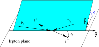
Figure 1: The Collins-Soper frame.

II The formalism for the Drell-Yan cross section

In the following, we will just sketch the kinematics and the necessary formulae for describing the $H_{1}H_{2}^{\uparrow}\to l^{+}l^{-}X$ cross section at leading twist. We forward the interested reader to Ref. Bianconi and Radici (2006b) for the technical details.

In the collision of two hadrons with momentum $P_{1},P_{2}$, and masses $M_{1},M_{2}$, the center-of-mass (c.m.) square energy $s=(P_{1}+P_{2})^{2}$ is available to produce two leptons with momenta $k_{1},k_{2}$, and invariant mass $q^{2}\equiv M^{2}=(k_{1}+k_{2})^{2}$. In the limit $M^{2},s\rightarrow\infty$, while keeping the ratio $0\leq\tau=M^{2}/s\leq 1$ limited, a factorization theorem can be proven Collins et al. (1985) ensuring that the elementary mechanism proceeds through the annihilation of a parton and an antiparton into a virtual photon with time-like momentum $q^{2}$. The partons are characterized by fractional longitudinal momenta $x_{1},x_{2}$, and spatial trasverse components ${\bm{p}}_{i\scriptstyle T}$ with respect to the direction defined by ${\bm{P}}_{i}\,(i=1,2)$, respectively. Momentum conservation implies ${\bm{q}}_{\scriptstyle T}={\bm{p}}_{1\scriptstyle T}+{\bm{p}}_{2\scriptstyle T}$. If ${\bm{q}}_{\scriptstyle T}\neq 0$ the annihilation direction is not known. Hence, it is convenient to select the socalled Collins-Soper frame Collins and Soper (1977) described in Fig. 1. The final lepton pair is detected in the solid angle $(\theta,\phi)$, where, in particular, $\phi$ (and all other azimuthal angles) is measured in a plane perpendicular to the indicated lepton plane but containing $\hat{\bm{h}}={\bm{q}}_{\scriptstyle T}/|{\bm{q}}_{\scriptstyle T}|$.

The full expression of the leading-twist differential cross section can be written as Boer (1999)

$$\frac{d\sigma}{d\Omega dx_{1}dx_{2}d{\bm{q}}_{\scriptstyle T}} = \frac{d\sigma^{o}}{d\Omega dx_{1}dx_{2}d{\bm{q}}_{\scriptstyle T}}+\frac{d\Delta\sigma^{\uparrow}}{d\Omega dx_{1}dx_{2}d{\bm{q}}_{\scriptstyle T}}$$ (1)

$$= \frac{\alpha^{2}}{3Q^{2}}\,\sum_{q}\,e_{q}^{2}\,\Bigg{\{}A(y)\,{\cal F}\left[f_{1}^{q}(H_{1})\,f_{1}^{q}(H_{2})\right]$$

$$\mbox{\hskip 56.9055pt}+B(y)\,\cos 2\phi\,{\cal F}\left[\left(2\hat{\bm{h}}\cdot{\bm{p}}_{1\scriptstyle T}\,\hat{\bm{h}}\cdot{\bm{p}}_{2\scriptstyle T}-{\bm{p}}_{1\scriptstyle T}\cdot{\bm{p}}_{2\scriptstyle T}\right)\,\frac{h_{1}^{\perp\,q}(H_{1})\,h_{1}^{\perp\,q}(H_{2})}{M_{1}\,M_{2}}\,\right]\Bigg{\}}$$

$$+\frac{\alpha^{2}}{3Q^{2}}\,|{\bm{S}}_{2\scriptstyle T}|\,\sum_{q}\,e_{q}^{2}\,\Bigg{\{}A(y)\,\sin(\phi-\phi_{S_{2}})\,{\cal F}\left[\hat{\bm{h}}\cdot{\bm{p}}_{2\scriptstyle T}\,\frac{f_{1}^{q}(H_{1})\,f_{1\scriptstyle T}^{\perp\,q}(H_{2}^{\uparrow})}{M_{2}}\right]$$

$$\mbox{\hskip 85.35826pt}-B(y)\,\sin(\phi+\phi_{S_{2}})\,{\cal F}\left[\hat{\bm{h}}\cdot{\bm{p}}_{1\scriptstyle T}\,\frac{h_{1}^{\perp\,q}(H_{1})\,h_{1}^{q}(H_{2}^{\uparrow})}{M_{1}}\right]$$

$$\mbox{\hskip 85.35826pt}-B(y)\,\sin(3\phi-\phi_{S_{2}})\,{\cal F}\left[\left(4\hat{\bm{h}}\cdot{\bm{p}}_{1\scriptstyle T}\,(\hat{\bm{h}}\cdot{\bm{p}}_{2\scriptstyle T})^{2}-2\hat{\bm{h}}\cdot{\bm{p}}_{2\scriptstyle T}\,{\bm{p}}_{1\scriptstyle T}\cdot{\bm{p}}_{2\scriptstyle T}-\hat{\bm{h}}\cdot{\bm{p}}_{1\scriptstyle T}\,{\bm{p}}_{2\scriptstyle T}^{2}\right)\right.$$

$$\mbox{\hskip 199.16928pt}\left.\times\frac{h_{1}^{\perp\,q}(H_{1})\,h_{1\scriptstyle T}^{\perp\,q}(H_{2}^{\uparrow})}{2M_{1}\,M_{2}^{2}}\,\right]\,\Bigg{\}}\;,$$

where $\alpha$ is the fine structure constant, $d\Omega=\sin\theta d\theta d\phi$, $e_{q}$ is the charge of the parton with flavor $q$, $\phi_{S_{i}}$ is the azimuthal angle of the transverse spin of hadron $i$, and

$$A(y)=\left(\frac{1}{2}-y+y^{2}\right)\,\stackrel{{\scriptstyle\mbox{cm}}}{{=}}\,\frac{1}{4}\left(1+\cos^{2}\theta\right) \mbox{\hskip 56.9055pt}B(y)=y(1-y)\,\stackrel{{\scriptstyle\mbox{cm}}}{{=}}\,\frac{1}{4}\,\sin^{2}\theta\;.$$ (2)

The convolutions are defined as

$${\cal F}\left[DF_{1}^{q}(H_{1})\,DF_{2}^{q}(H_{2}^{(\uparrow)})\right]\equiv\int d{\bm{p}}_{1\scriptstyle T}d{\bm{p}}_{2\scriptstyle T}\,\delta\left({\bm{p}}_{1\scriptstyle T}+{\bm{p}}_{2\scriptstyle T}-{\bm{q}}_{\scriptstyle T}\right)\,\left[DF_{1}(x_{1},{\bm{p}}_{1\scriptstyle T};\bar{q}/H_{1})\,DF_{2}(x_{2},{\bm{p}}_{2\scriptstyle T};q/H_{2}^{(\uparrow)})+(q\leftrightarrow\bar{q})\right]\;.$$ (3)

Parton distribution functions can be obtained from the color-gauge invariant quark-quark correlator

$$\Phi(x,S)=\int\frac{d\xi^{-}}{2\pi}\,e^{ixP^{+}\xi^{-}}\,\langle P,S|\bar{\psi}(0)\,U_{[0,\xi^{-}]}\,\psi(\xi)|P,S\rangle\Bigg{|}_{\xi^{+}={\bm{\xi}}_{\scriptstyle T}=0}\;,$$ (4)

where

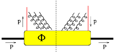
Figure 2: A possible representation of the color-gauge invariant quark-quark correlator.

$$U_{[0,\xi]}={\cal P}\,e^{-ig\int_{0}^{\xi}dw\cdot A(w)}$$ (5)

is the socalled gauge link operator, connecting the two different space-time points $0,\xi,$ by all the possible ordered paths (${\cal P}[..]$) followed by the gluon field $A$, which couples to the quark field $\psi$ through the constant $g$. Only $A^{+}$ gluons appear at any power in the expansion of the exponential, leading to an intuitive representation of the gauge link operator as a sort of residual interaction between the parton and the residual hadron (see Fig. 2). When also including the ${\bm{p}}_{\scriptstyle T}$ dependence in Eq. 4, the integration path of the gauge link is more complicated and involves ${\bm{A}}_{\scriptstyle T}$ gluons at light-cone infinity Bomhof et al. (2004). For the specific case of interest of hadrons with transverse polarization ${\bm{S}}_{\scriptstyle T}$, the quark-quark correlator can be parametrized as

$$\Phi(x,{\bm{p}}_{\scriptstyle T},S_{\scriptstyle T}) = \frac{1}{2P^{+}}\,\left\{f_{1}(x,{\bm{p}}_{\scriptstyle T})\,\kern 1.99997ptP\kern-5.0pt/+f_{1\scriptstyle T}^{\perp}(x,{\bm{p}}_{\scriptstyle T})\,\epsilon_{\mu\nu\rho\sigma}\,\gamma^{\mu}\,\frac{P^{\nu}p^{\rho}S_{\scriptstyle T}^{\sigma}}{M_{H}}+h_{1}^{\perp}(x,{\bm{p}}_{\scriptstyle T})\,\sigma_{\mu\nu}\,\frac{p^{\mu}P^{\nu}}{M_{H}}\right.$$ (6)

$$\left.-h_{1}(x,{\bm{p}}_{\scriptstyle T})\,i\sigma_{\mu\nu}\,S_{\scriptstyle T}^{\mu}P^{\nu}\,\gamma_{5}-h_{1\scriptstyle T}^{\perp}(x,{\bm{p}}_{\scriptstyle T})\,\left(\frac{{\bm{p}}_{\scriptstyle T}\cdot{\bm{S}}_{\scriptstyle T}}{M_{H}}\,\frac{p^{\mu}P^{\nu}}{M_{H}}-\frac{{\bm{p}}_{\scriptstyle T}^{2}}{M_{H}^{2}}\,S_{\scriptstyle T}^{\mu}P^{\nu}\right)\,i\sigma_{\mu\nu}\,\gamma_{5}\right\}\;,$$

where $M_{H}$ is the parent hadron mass.

The TMD functions of Eq. (1) can thus be obtained by suitable projections

$$\Phi^{\left[\Gamma\right]}(x,{\bm{p}}_{\scriptstyle T},{\bm{S}}_{\scriptstyle T})=\frac{1}{2}\int dp^{-}\,\mathrm{Tr}\left[\Gamma\,\Phi(p,P,{\bm{S}}_{\scriptstyle T})\right]\Bigg{|}_{p^{+}=xP^{+}}\;.$$ (7)

In fact, following Ref. Bacchetta et al. (2004a) we can define the number density $f_{qs_{T}/HS_{T}}$ of partons with flavor $q$ and transverse polarization $s_{\scriptstyle T}$ in a hadron $H$ with transverse polarization $S_{\scriptstyle T}$:

$$f_{qs_{T}/HS_{T}} = \frac{1}{2}\,\left(\Phi^{[\kern 1.39998ptn\kern-3.5pt/_{\scriptscriptstyle-}/2]}+\Phi^{[i\sigma_{\mu\nu}\,n_{\scriptscriptstyle-}^{\mu}s^{\nu}\gamma_{5}/2]}\right)$$ (8)

$$= \frac{1}{4}\,\left\{f_{1}^{q}(x,{\bm{p}}_{\scriptstyle T})-f_{1\scriptstyle T}^{\perp\,q}(x,{\bm{p}}_{\scriptstyle T})\,\frac{\hat{{\bm{P}}}\times{\bm{p}}_{\scriptstyle T}\cdot{\bm{S}}_{\scriptstyle T}}{M_{H}}-h_{1}^{\perp\,q}(x,{\bm{p}}_{\scriptstyle T})\,\frac{\hat{{\bm{P}}}\times{\bm{p}}_{\scriptstyle T}\cdot{\bm{s}}_{\scriptstyle T}}{M_{H}}\right.$$

$$\left.+h_{1}^{q}(x,{\bm{p}}_{\scriptstyle T})\,{\bm{S}}_{\scriptstyle T}\cdot{\bm{s}}_{\scriptstyle T}+h_{1\scriptstyle T}^{\perp\,q}(x,{\bm{p}}_{\scriptstyle T})\,\left(\frac{{\bm{p}}_{\scriptstyle T}\cdot{\bm{S}}_{\scriptstyle T}}{M_{H}}\,\frac{{\bm{p}}_{\scriptstyle T}\cdot{\bm{s}}_{\scriptstyle T}}{M_{H}}\,-\frac{{\bm{p}}_{\scriptstyle T}^{2}}{M_{H}^{2}}\,{\bm{S}}_{\scriptstyle T}\cdot{\bm{s}}_{\scriptstyle T}\right)\right\}\;,$$

where $n_{-}=(1,0,{\bm{0}}_{\scriptstyle T})$. It is easy to verify that the unpolarized parton distribution is obtained by summing the number densities for all possible four combinations of transverse polarizations: $f_{1}^{q}=f_{q\uparrow/H\uparrow}+f_{q\downarrow/H\uparrow}+f_{q\uparrow/H\downarrow}+f_{q\downarrow/H\downarrow}$. Similarly, the Sivers function emerges as the unbalance between the probabilities of finding unpolarized partons inside hadrons transversely polarized in opposite directions, namely

$$(f_{q\uparrow/p\uparrow}+f_{q\downarrow/p\uparrow})-(f_{q\uparrow/p\downarrow}+f_{q\downarrow/p\downarrow})=f_{q/p\uparrow}-f_{q/p\downarrow}=-f_{1\scriptstyle T}^{\perp\,q}(x,{\bm{p}}_{\scriptstyle T})\,\frac{\hat{\bm{P}}\times{\bm{p}}_{\scriptstyle T}\cdot{\bm{S}}_{\scriptstyle T}}{M_{H}}\;.$$ (9)

The Boer-Mulders function and the transversity emerge from the other two combinations

$$(f_{q\uparrow/p\uparrow}+f_{q\uparrow/p\downarrow})-(f_{q\downarrow/p\uparrow}+f_{q\downarrow/p\downarrow}) = f_{q\uparrow/p}-f_{q\downarrow/p}=-h_{1\scriptstyle T}^{\perp\,q}(x,{\bm{p}}_{\scriptstyle T})\,\frac{\hat{\bm{P}}\times{\bm{p}}_{\scriptstyle T}\cdot{\bm{s}}_{\scriptstyle T}}{M_{H}}\;,$$ (10)

$$(f_{q\uparrow/p\uparrow}-f_{q\uparrow/p\downarrow})-(f_{q\downarrow/p\uparrow}-f_{q\downarrow/p\downarrow}) = h_{1}^{q}(x,{\bm{p}}_{\scriptstyle T})\,{\bm{S}}_{\scriptstyle T}\cdot{\bm{s}}_{\scriptstyle T}+h_{1\scriptstyle T}^{\perp\,q}(x,{\bm{p}}_{\scriptstyle T})\,\left(\frac{{\bm{p}}_{\scriptstyle T}\cdot{\bm{S}}_{\scriptstyle T}\,{\bm{p}}_{\scriptstyle T}\cdot{\bm{s}}_{\scriptstyle T}}{M_{H}^{2}}-\frac{{\bm{p}}_{\scriptstyle T}^{2}}{M_{H}^{2}}\,{\bm{S}}_{\scriptstyle T}\cdot{\bm{s}}_{\scriptstyle T}\right)\;.$$ (11)

III Monte Carlo generation of Drell-Yan events

The implementation of Eq. (1) in the Monte Carlo generator is represented as Bianconi and Radici (2005a):

$$\frac{d\sigma}{d\Omega dx_{1}dx_{2}d{\bm{q}}_{\scriptstyle T}}=K\,\frac{1}{s}\,|{\cal T}({\bm{q}}_{\scriptstyle T},x_{1},x_{2},M)|^{2}\,\sum_{i=1}^{3}\,c_{i}({\bm{q}}_{\scriptstyle T},x_{1},x_{2})\,S_{i}(\theta,\phi,\phi_{{}_{S_{2}}})\;,$$ (12)

where the event distribution is driven by the elementary unpolarized annihilation $|{\cal T}|^{2}$. We assume a factorized transverse-momentum dependence in each parton distribution such as to break the convolution ${\cal F}$ in Eq.(3), leading to

$$|{\cal T}|^{2}\approx A(q_{\scriptstyle T},x_{1},x_{2},M)\,F(x_{1},x_{2})\;,$$ (13)

where $q_{\scriptstyle T}\equiv|{\bm{q}}_{\scriptstyle T}|$. The function $A$ is parametrized and normalized as in Ref. Conway et al. (1989), where high-energy Drell-Yan $\pi-p$ collisions were considered. The average transverse momentum turns out to be $\langle q_{\scriptstyle T}\rangle>1$ GeV/$c$, which effectively reproduces the influence of sizable QCD corrections beyond the parton model picture of Eq. (1). It is well known Altarelli et al. (1979) that such corrections induce also large $K$ factors and an $M$ scale dependence in parton distributions, determining their evolution. As in our previous works Bianconi and Radici (2005a, 2006a, c, 2006b), we conventionally assume in Eq. (12) that $K=2.5$, but we stress that in an azimuthal asymmetry the corrections to the cross sections in the numerator and in the denominator should approximately compensate each other, as it turns out to happen at RHIC Martin et al. (1998) and JPARC Kawamura et al. (2007) c.m. energies. Since the range of $M$ values here explored is close to the one of Ref. Conway et al. (1989), where the parametrization of $A,F,$ and $c_{i}$ in Eq. (12) was deduced assuming $M$-independent parton distributions, we keep our same previous approach Bianconi and Radici (2005a, 2006a, c, 2006b) and use

$$F(x_{1},x_{2})=\frac{\alpha^{2}}{12Q^{2}}\,\sum_{q}\,e_{q}^{2}\,f_{1}^{q}(x_{1};\bar{q}/H_{1})\,f_{1}^{q}(x_{2};q/H_{2})+(\bar{q}\leftrightarrow q)\;,$$ (14)

where the unpolarized distribution $f_{1}^{q}(x)$ for various flavors $q=u,d,s,$ is taken again from Ref. Conway et al. (1989), unless an explicit different choice is mentioned.

The whole solid angle $(\theta,\phi)$ of the final lepton pair in the Collins-Soper frame is randomly distributed in each variable. The explicit form for sorting it in the Monte-Carlo is Bianconi and Radici (2005a, 2006a, 2006b)

$$\sum_{i=1}^{3}\,c_{i}(q_{\scriptstyle T},x_{1},x_{2})\,S_{i}(\theta,\phi,\phi_{S_{2}}) = (1+\cos^{2}\theta)+\frac{\nu(x_{1},x_{2},q_{\scriptstyle T})}{2}\,\sin^{2}\theta\,\cos 2\phi$$ (15)

$$+|{\bm{S}}_{2\scriptstyle T}|\,c_{3}(q_{\scriptstyle T},x_{1},x_{2})\,S_{3}(\theta,\phi,\phi_{S_{2}})\;.$$

If quarks were massless, the virtual photon would be only transversely polarized and the angular dependence would be described by the coefficient $c_{1}=1,\,S_{1}=1+\cos^{2}\theta$. In the following, we discuss violations of such azimuthally symmetric dependence, as they appear in Eq. (15).

III.1 The $\cos 2\phi$ asymmetry

Azimuthal $\cos 2\phi$ asymmetries in Eq. (12), induced by $c_{2}\equiv\textstyle{\frac{\nu}{2}}$, are due to the longitudinal polarization of the virtual photon and to the fact that quarks have an intrinsic transverse momentum distribution, leading to the explicit violation of the socalled Lam-Tung sum rule Conway et al. (1989). QCD corrections influence $\nu$, which in principle depends also on $M^{2}$ Conway et al. (1989). The coefficient $c_{2}$ was simulated at the GSI kinematics Bianconi and Radici (2005a), using the simple parametrization of Ref. Boer (1999) and testing it against the previous measurement of Ref. Guanziroli et al. (1988). The ${\bm{p}}_{\scriptstyle T}$ dependence of the parton distributions in the nucleon was parametrized as Boer (1999)

$$f_{1}^{q}(x,{\bm{p}}_{\scriptstyle T}) = \frac{\alpha_{\scriptstyle T}}{\pi}\,e^{-\alpha_{\scriptstyle T}\,{\bm{p}}_{\scriptstyle T}^{2}}\,f_{1}^{q}(x)$$

$$h_{1}^{\perp\,q}(x,{\bm{p}}_{\scriptstyle T}) = c^{q}\,\frac{M_{{}_{C}}\,M_{N}}{{\bm{p}}_{\scriptstyle T}^{2}+M_{{}_{C}}^{2}}\,f_{1}^{q}(x,{\bm{p}}_{\scriptstyle T})\;,$$ (16)

where $\alpha_{\scriptstyle T}=1$ GeV^-2, $M_{{}_{C}}=2.3$ GeV, $c^{q}=1$, and $M_{N}$ is the nucleon mass. Following the steps in Sec. VI of Ref. Boer (1999), one easily gets

$$c_{2}^{\nu} \equiv \frac{\nu}{2}=\frac{\sum_{q}\,e_{q}^{2}\,{\cal F}\left[\left(2\hat{\bm{h}}\cdot{\bm{p}}_{1\scriptstyle T}\,\hat{\bm{h}}\cdot{\bm{p}}_{2\scriptstyle T}-{\bm{p}}_{1\scriptstyle T}\cdot{\bm{p}}_{2\scriptstyle T}\right)\,\displaystyle{\frac{\bar{h}_{1}^{\perp\,q}(x_{1},{\bm{p}}_{1\scriptstyle T})\,h_{1}^{\perp\,q}(x_{2},{\bm{p}}_{2\scriptstyle T}}{M_{1}\,M_{2}}}\,\right]+(1\leftrightarrow 2)}{\sum_{q}\,e_{q}^{2}\,{\cal F}\left[\bar{f}_{1}^{q}(x_{1},{\bm{p}}_{1\scriptstyle T})\,f_{1}^{q}(x_{2},{\bm{p}}_{2\scriptstyle T})\right]+(1\leftrightarrow 2)}$$ (17)

$$\approx \frac{4M_{C}^{2}\,q_{\scriptstyle T}^{2}}{(q_{\scriptstyle T}^{2}+4M_{C}^{2})^{2}}\;.$$

Since the ${\bm{p}}_{\scriptstyle T}$ dependence of $h_{1}^{\perp}$ was fitted to the measured $\cos 2\phi$ asymmetry of the corresponding unpolarized Drell-Yan cross section, which is small for $1\lesssim q_{\scriptstyle T}\lesssim 3$ GeV/$c$ (see, for example, Fig.4 in Ref. Boer (1999)), correspondingly, the $\cos 2\phi$ asymmetry turned out to be small for the considered statistically relevant $q_{\scriptstyle T}$ range in kinematics conditions reachable at GSI Bianconi and Radici (2005a).

In the literature, there are several models available for $h_{1}^{\perp}$ in the nucleon; in particular, in the context of the spectator diquark model both T-even Jakob et al. (1997) and T-odd parton densities Brodsky et al. (2002) have been analyzed, and further work is in progress Gamberg et al. (2007). Here, we reconsider the spectator diquark model of Ref. Bacchetta et al. (2004b) and we present some preliminary results, obtained in the context of an improved and enlarged approach Bacchetta et al. (2007a). The main features of the latter are the following. The gauge link appearing in the quark-quark correlator is expanded and truncated at the one-gluon exchange level (see Fig. 2). The emerging interference diagrams produce the naive T-odd structures necessary to have nonvanishing TMD distributions like the Sivers $f_{1\scriptstyle T}^{\perp}$ and the Boer-Mulders $h_{1}^{\perp}$ functions. Because of the symmetry properties of the nucleon wave function, scalar and axial-vector diquarks are considered with different couplings to the valence quark left. A dipole-like form factor is attached at each nucleon-quark-diquark vertex (but other choices will be explored Bacchetta et al. (2007a)). The obtained expressions, that replace the ones in Eq. (16), are

$$f_{1}^{q}(x,{\bm{p}}_{\scriptstyle T}) = \frac{N_{qS}^{2}}{16\pi^{3}}\,\frac{\left[{\bm{p}}_{\scriptstyle T}^{2}+(m+M_{N}x)^{2}\right]\,(1-x)^{3}}{\left(A_{S}^{2}+{\bm{p}}_{\scriptstyle T}^{2}\right)^{4}}+\frac{N_{qa}^{2}}{16\pi^{3}}\,\frac{\left[{\bm{p}}_{\scriptstyle T}^{2}(1+x^{2})+(m+M_{N}x)^{2}(1-x)^{2}\right]\,(1-x)}{\left(A_{a}^{2}+{\bm{p}}_{\scriptstyle T}^{2}\right)^{4}}$$

$$h_{1}^{\perp\,q}(x,{\bm{p}}_{\scriptstyle T}) = \frac{N_{qS}^{2}}{64\pi^{4}}\,ee_{D}\,\frac{M_{N}(m+M_{N}x)\,(1-x)^{3}}{A_{S}^{2}\,\left(A_{S}^{2}+{\bm{p}}_{\scriptstyle T}^{2}\right)^{3}}+\frac{N_{qa}^{2}}{64\pi^{4}}\,ee_{D}\,\frac{M_{N}(m+M_{N}x)\,(1-x)^{2}}{A_{a}^{2}\,\left(A_{a}^{2}+{\bm{p}}_{\scriptstyle T}^{2}\right)^{3}}\;,$$ (18)

where

$$A_{S/a}^{2}=(1-x)\Lambda^{2}+xM_{S/a}^{2}-x(1-x)M_{N}^{2}\;,\quad ee_{D}=-4\pi\,C_{F}\,\alpha_{s}\approx-\frac{16\pi}{3}\,0.3\;,$$ (19)

and $m=0.36$ GeV is the valence (constituent) quark mass, $\Lambda=0.5$ is a cutoff for high quark virtualities, $M_{S}=0.6$ GeV and $M_{a}=0.8$ GeV are the scalar and axial-vector diquark masses, respectively. With these choices, the normalizations turn out to be $N_{uS}^{2}=6.52\times 3/2,\,N_{ua}^{2}=30.63\times 1/2,\,N_{dS}^{2}=0,\,N_{da}^{2}=30.63$. The sign of the obtained $h_{1}^{\perp\,q}$ (and also of $f_{1\scriptstyle T}^{\perp\,q}$, see below) is consistent with the lattice predictions Gockeler et al. (2006) for both $q=u,d$.

As a preliminary step in the analysis of azimuthal asymmetries at COMPASS, for the evolution of the parton densities in this context we made an educated guess, since this information is unknown for both $f_{1\scriptstyle T}^{\perp}$ and $h_{1}^{\perp}$. We have integrated the ${\bm{p}}_{\scriptstyle T}$ dependence away in Eq. (18), and applied DGLAP evolution at NLO using the code of Ref. Miyama and Kumano (1996) for unpolarized quarks and of Ref. Hirai et al. (1998) for transversely polarized ones. The resulting expressions have been inserted in Eq. (16) in place of the corresponding $f_{1}^{q}(x)$, in order to have an evolved model dependence in the behaviour in $x$, but retaining the phenomenological behaviour in ${\bm{p}}_{\scriptstyle T}$ fitted to the available data. Consistently with the discussed approximations, also the evolution scales have been determined in an approximate way. The final scale obviously reflects the foreseen COMPASS setup, where Drell-Yan dileptons can be detected with invariant masses above 4 GeV; hence, DGLAP evolution has been stopped at $Q^{2}=16$ GeV². The initial soft scale has been deduced by solving the renormalization group equations for the second Mellin moment of the non-singlet (valence) distribution, with the anomalous dimension consistently determined at NLO; the result is $Q_{0}^{2}\approx 0.1$ GeV². In Fig. 3 the model $xh_{1}^{\perp\,u}(x)$ is shown at $Q_{0}^{2}$ (blue line) and at $Q^{2}$ (black line); the red line is a fit to the latter one with the form $Nx^{\alpha}(1-x)^{\beta}$, which is actually used in the Monte Carlo calculation of the coefficient $c_{2}^{\nu}$ to produce the azimuthal asymmetry.

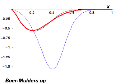
Figure 3: The spectator diquark model calculation of the Boer-Mulders function $xh_{1}^{\perp\,u}(x)$ at two different scales: initial $Q_{0}^{2}=0.1$ GeV² (blue line), final $Q^{2}=16$ GeV² (black line). DGLAP evolution is considered at NLO level. The red line is a 3-parameter fit to the black line (see text).

III.2 The Sivers effect

If we consider the Sivers effect in Eq. (1), the last term in Eq. (15) becomes

$$S_{3}^{\mathrm{Siv}}(\theta,\phi,\phi_{S_{2}})=(1+\cos^{2}\theta)\,\sin(\phi-\phi_{S_{2}})$$ (20)

and the corresponding coefficient $c_{3}$ reads

$$c_{3}^{\mathrm{Siv}}(q_{\scriptstyle T},x_{1},x_{2})=\frac{\sum_{q}\,e_{q}^{2}\,{\cal F}\left[\hat{\bm{h}}\cdot{\bm{p}}_{2\scriptstyle T}\,\displaystyle{\frac{f_{1}^{q}(x_{1},{\bm{p}}_{1\scriptstyle T})\,f_{1\scriptstyle T}^{\perp\,q}(x_{2},{\bm{p}}_{2\scriptstyle T})}{M_{2}}}\right]}{\sum_{q}\,e_{q}^{2}\,{\cal F}\left[f_{1}^{q}(x_{1},{\bm{p}}_{1\scriptstyle T})\,f_{1}^{q}(x_{2},{\bm{p}}_{2\scriptstyle T})\right]}\;,$$ (21)

where the complete dependence of the involved TMD parton distributions has been made explicit. For the Sivers function $f_{1\scriptstyle T}^{\perp}$, we adopt the parametrization described in Ref. Bianconi and Radici (2006a). It is inspired to the one of Ref. Vogelsang and Yuan (2005), where the transverse momentum of the detected pion in the SIDIS process was assumed to come entirely from the ${\bm{p}}_{\scriptstyle T}$ dependence of the Sivers function, and was further integrated out building the fit in terms of specific moments of the function itself. The $x$ dependence of that approach is here retained, but a different flavor-dependent normalization and an explicit ${\bm{p}}_{\scriptstyle T}$ dependence are introduced that are bound to the shape of the recent RHIC data on $pp^{\uparrow}\to\pi X$ at $\sqrt{s}=200$ GeV Adler et al. (2005), where large persisting asymmetries are found that could be partly due to the leading-twist Sivers mechanism. The expression adopted is

$$f_{1\scriptstyle T}^{\perp\,q}(x,{\bm{p}}_{\scriptstyle T}) = N_{q}\,x\,(1-x)\,\frac{M_{2}p_{0}^{2}p_{\scriptstyle T}}{(p_{\scriptstyle T}^{2}+\frac{p_{0}^{2}}{4})^{2}}\,f_{1}^{q}(x,{\bm{p}}_{\scriptstyle T})$$ (22)

$$= N_{q}\,x\,(1-x)\,\frac{M_{2}p_{0}^{2}p_{\scriptstyle T}}{(p_{\scriptstyle T}^{2}+\frac{p_{0}^{2}}{4})^{2}}\,\frac{1}{\pi\,\langle p_{\scriptstyle T}^{2}\rangle}\,e^{-p_{\scriptstyle T}^{2}/\langle p_{\scriptstyle T}^{2}\rangle}\,f_{1}^{q}(x)\;,$$

where $p_{0}=2$ GeV/$c$, and $N_{u}=-N_{d}=0.7$. The sign, positive for $u$ quarks and negative for the $d$ ones, already takes into account the predicted sign change of $f_{1\scriptstyle T}^{\perp}$ from Drell-Yan to SIDIS Collins (2002).

Following the steps described in Sec. III-2 of Ref. Bianconi and Radici (2006a), we can directly insert Eq. (22) into Eq. (21) and get

$$c_{3}^{\mathrm{Siv}}\approx x_{2}\,(1-x_{2})\,\left(\frac{2\,p_{0}\,q_{\scriptstyle T}}{q_{\scriptstyle T}^{2}+p_{0}^{2}}\right)^{2}\,\frac{8\,N_{u}+N_{d}}{9}\;.$$ (23)

The $q_{\scriptstyle T}$ shape and peak position are in agreement with a similar analysis of the azimuthal asymmetry of the unpolarized Drell-Yan data (the violation of the Lam-Tung sum rule Boer (1999)), but are induced also by the observed $x_{{}_{F}}-q_{\scriptstyle T}$ correlation in the above mentioned RHIC data for $pp^{\uparrow}\to\pi X$, when it is assumed that the SSA is entirely due to the Sivers mechanism. This suggests that the maximum asymmetry is reached in the upper valence region such that $x_{{}_{F}}\approx x_{2}\sim\langle q_{\scriptstyle T}\rangle/5$ Adler et al. (2005).

III.3 The Boer-Mulders effect

If we consider the Boer-Mulders effect in Eq. (1), the last term in Eq. (15) becomes

$$S_{3}^{\mathrm{BM}}(\theta,\phi,\phi_{S_{2}})=\sin^{2}\theta\,\sin(\phi+\phi_{S_{2}})$$ (24)

and the corresponding coefficient $c_{3}$ reads

$$c_{3}^{\mathrm{BM}}(q_{\scriptstyle T},x_{1},x_{2})=-\frac{\sum_{q}\,e_{q}^{2}\,{\cal F}\left[\hat{\bm{h}}\cdot{\bm{p}}_{1\scriptstyle T}\,\displaystyle{\frac{h_{1}^{\perp\,q}(x_{1},{\bm{p}}_{1\scriptstyle T})\,h_{1}^{q}(x_{2},{\bm{p}}_{2\scriptstyle T})}{M_{1}}}\right]}{\sum_{q}\,e_{q}^{2}\,{\cal F}\left[f_{1}^{q}(x_{1},{\bm{p}}_{1\scriptstyle T})\,f_{1}^{q}(x_{2},{\bm{p}}_{2\scriptstyle T})\right]}\;.$$ (25)

As in Ref. Boer (1999), one can use Eq. (16) and the following parametrization for transversity,

$$h_{1}^{q}(x,{\bm{p}}_{\scriptstyle T})=\frac{\alpha_{\scriptstyle T}}{\pi}\,e^{-\alpha_{\scriptstyle T}\,{\bm{p}}_{\scriptstyle T}^{2}}\,h_{1}^{q}(x)\;,$$ (26)

to get

$$c_{3}^{\mathrm{BM}} = -\frac{2M_{{}_{C}}\,q_{\scriptstyle T}}{q_{\scriptstyle T}^{2}+4M_{{}_{C}}^{2}}\,\frac{\sum_{q}\,e_{q}^{2}\,f_{1}^{q}(x_{1};\bar{q}/H_{1})\,h_{1}^{q}(x_{2};q/H_{2}^{\uparrow})+(\bar{q}\leftrightarrow q)}{\sum_{q}\,e_{q}^{2}\,f_{1}^{q}(x_{1};\bar{q}/H_{1})\,f_{1}^{q}(x_{2};q/H_{2})+(\bar{q}\leftrightarrow q)}$$ (27)

$$\approx -\frac{2M_{{}_{C}}\,q_{\scriptstyle T}}{q_{\scriptstyle T}^{2}+4M_{{}_{C}}^{2}}\,\frac{f(x_{1};\langle\bar{q}\rangle/H_{1})\,h_{1}(x_{2};\langle q\rangle/H_{2}^{\uparrow})}{f(x_{1};\langle\bar{q}\rangle/H_{1})\,f_{1}(x_{2};\langle q\rangle/H_{2})}\equiv-\frac{2M_{{}_{C}}\,q_{\scriptstyle T}}{q_{\scriptstyle T}^{2}+4M_{{}_{C}}^{2}}\,\frac{h_{1}(x_{2};\langle q\rangle/H_{2}^{\uparrow})}{f_{1}(x_{2};\langle q\rangle/H_{2})}\;,$$

where the second step is justified by assuming that the contribution of each flavor to each parton distribution can be approximated by a corresponding average function. This approximation, together with the systematic neglect of sea (anti)quark contributions, has been widely explored in Ref. Bianconi and Radici (2007), and it turns out to be largely justified at COMPASS kinematics. Because of the lack of parametrizations for $h_{1}^{\perp}$, numerical simulations of $c_{3}^{\mathrm{BM}}$ were performed in Ref. Bianconi and Radici (2006b) by making two different guesses for the ratio $h_{1}(x_{2};\langle q\rangle/H_{2}^{\uparrow})/f_{1}(x_{2};\langle q\rangle/H_{2})$, namely the ascending function $\sqrt{x_{2}}$ and the descending one $\sqrt{1-x_{2}}$, that both respect the Soffer bound. The goal was to determine the minimum number of events (compatible with the kinematical setup and cuts) required to produce azimuthal asymmetries that could be clearly distinguished like the corresponding originating distributions.

Alternatively, here we will show preliminary results for the $c_{3}^{\mathrm{BM}}$ asymmetry obtained in the spectator diquark model Bacchetta et al. (2007a) by using the same strategy discussed in Sec. III.1. Namely, we start from the ${\bm{p}}_{\scriptstyle T}$-integrated model expressions for $f_{1}^{q}$ and $h_{1}^{\perp\,q}$ from Eq. (18), complemented by the model transversity

$$h_{1}^{q}(x)=\frac{N_{qS}^{2}}{48\pi^{2}}\,\frac{(m+M_{N}x)^{2}\,(1-x)^{3}}{A_{S}^{6}}-\frac{N_{qa}^{2}}{48\pi^{2}}\,\frac{x(1-x)}{A_{a}^{4}}\;.$$ (28)

Next, we evolve these distributions from $Q_{0}^{2}=0.1$ GeV² to $Q^{2}=16$ GeV² with a (polarized) DGLAP NLO kernel. Then, we fit each result with different 3-parameter forms $N_{i}x^{\alpha_{i}}(1-x)^{\beta_{i}},\,i=1-3$, and we replace them in the corresponding $x$-dependent part of the parametrizations (16) and (26). The calculation of $c_{3}^{\mathrm{BM}}$ then develops in the same way up to the first line of Eq. (27), where each $x$-dependent parton density is now replaced by its properly-evolved corresponding expression in the spectator diquark model, with no need to apply the flavor average approximation. Note that the $f_{1}^{q}$ in the numerator now does not simplify with the one in the denominator, because the former and the latter are replaced by the ${\bm{p}}_{\scriptstyle T}$-integrated and evolved $h_{1}^{\perp\,q}(x,{\bm{p}}_{\scriptstyle T})$ and $f_{1}^{q}(x,{\bm{p}}_{\scriptstyle T})$ functions of Eq. (18), respectively.

IV Results of Drell-Yan Monte Carlo simulations

In the Monte Carlo simulation, events are generated by Eq. (13), and azimuthal asymmetries are produced by Eq. (17) for the $\cos 2\phi$ asymmetry in unpolarized Drell-Yan, by Eq. (23) for the Sivers effect, and by Eq. (27) for the Boer-Mulders effect, respectively, using phenomenological parametrizations or model inputs for the involved (TMD) parton densities, as it is described in the previous section. The general strategy is to divide the event sample in two groups, one for positive values ”$U$” of $S_{2}=\sin^{2}\theta\cos 2\phi$ in the unpolarized cross section (or of $S_{3}^{\mathrm{Siv}}=(1+\cos^{2}\theta)\sin(\phi-\phi_{S_{2}})$ for Sivers effect, or $S_{3}^{\mathrm{BM}}=\sin^{2}\theta\sin(\phi+\phi_{S_{2}})$ for the Boer-Mulders effect), and another one for negative values ”$D$”, then taking the ratio $(U-D)/(U+D)$ Bianconi and Radici (2005a). Data are accumulated only in the $x_{2}$ bins of the polarized proton, i.e. they are summed over in the $x_{1}$ bins for the beam, in the transverse momentum $q_{\scriptstyle T}$ of the muon pair and in their zenithal orientation $\theta$. Statistical errors for the asymmetry $(U-D)/(U+D)$ are obtained by making 10 independent repetitions of the simulation for each individual case, and then calculating for each $x_{2}$ bin the average asymmetry value and the variance. We checked that 10 repetitions are a reasonable threshold to have stable numbers, since the results do not change significantly when increasing the number of repetitions beyond 6.

The transversely polarized proton target is obtained from a $NH_{3}$ molecule where each $H$ nucleus is fully transversely polarized and the number of ”polarized” collisions is 25% of the total number of collisions, i.e. with a dilution factor 1/4 Bianconi and Radici (2005a). The beam is represented by charged pions or antiprotons such that $100\leq s\leq 200$ GeV², i.e. roughly the c.m. energy available at GSI in the socalled asymmetric collider mode Bianconi and Radici (2005a). The reason for employing antiproton beams is simply due to the lack of knowledge of $h_{1}^{\perp}$ in the pion. Antiproton-proton collisions involve annihilations of valence parton densities, as do the pion-proton ones. Hence, it is anyway useful to study the shape and size of this asymmetry in the same kinematic conditions, even if this kind of projectile is presently not considered at COMPASS. The invariant mass of the lepton pair (usually, muons) is constrained in the $1.5<M<2.5$ GeV and $4<M<9$ GeV ranges, according to the value of $s$, in order to explore approximately the same $x$ valence range and to avoid overlaps with the resonance regions of the $\bar{c}c$ and $\bar{b}b$ quarkonium systems.

Proper cuts are applied to the $q_{\scriptstyle T}$ distribution, namely $1<q_{\scriptstyle T}<3$ GeV/$c$, in order to filter out low-$q_{\scriptstyle T}$ muon pairs from background processes other than the Drell-Yan mechanism, and to optimize the ratio between the absolute sizes of the asymmetry and the statistical errors. The resulting $\langle q_{\scriptstyle T}\rangle\sim 1.8$ GeV/$c$ is in fair agreement with the one experimentally explored at RHIC Adler et al. (2005). Whenever the $\theta$ angular dependence is represented by a $\sin^{2}\theta$ function, like for the $S_{2}$ of Eq. (15) and for the $S_{3}^{\mathrm{BM}}$ of Eq. (24), the angular distribution is constrained in the range $60^{\rm o}<\theta<120^{\rm o}$, because outside these limits the azimuthal asymmetry is too small Bianconi and Radici (2005a).

Table 1: Total absorption cross sections per nucleon and related Drell-Yan event counts per month, for pion- and antiproton-proton collisions at $s=200$ GeV² and luminosity ${\cal L}=4\times 10^{31}$ cm^-2s^-1, producing Drell-Yan pairs for various invariant masses (see text for a discussion of the kinematics and the cutoffs).

beam	$M$ (GeV)	$\sigma_{tot}$ (nb/nucleon)	events per month
$\pi$	2.5-4 (no $J/\psi$)	0.5	$52\,000$
$\pi$	4-9	0.25	$26\,000$
$\bar{p}$	1.5-2.5	2.4	$249\,600$
$\bar{p}$	4-9	0.1	$10\,400$

The above cuts typically produce a reduction factor of  2.5 in the initial event sample Bianconi and Radici (2005a). For pion beams, we can easily think of samples as large as $250\,000$ events, which are then reduced to $100\,000$, and further to $25\,000$ in polarized collisions by the target dilution factor. It is much more difficult to get these numbers using antiproton beams. However, in our simulation of $\bar{p}p^{\left(\uparrow\right)}\to\mu^{+}\mu^{-}X$ processes we will keep them in order to make consistent statistical comparisons with the pion beam case. In Tab.1, we list several values of the total absorption cross section $\sigma_{\mathrm{tot}}$ per single nucleon, as they are deduced from our Monte Carlo for pion and antiproton beams hitting a $NH_{3}$ target at $s=200$ GeV² and in the above specified conditions, and producing final Drell-Yan muons with different invariant masses. At the luminosity ${\cal L}=4\times 10^{31}$ cm^-2s^-1 and with efficiency 1, the product $\sigma_{tot}{\cal L}$ gives the number of Drell-Yan events per nucleon and per second that could be ideally reached at COMPASS. For example, with pion beams of 100 GeV energy hitting a transversely polarized $NH_{3}$ target at $s=200$ GeV², and producing muon pairs with invariant masses in the range 4-9 GeV, it is possible to collect around $25\,000$ Drell-Yan events within approximately one month of run at the luminosity $4\times 10^{31}$ cm^-2s^-1.

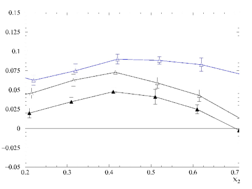
Figure 4: The asymmetry $(U-D)/(U+D)$ with positive ($U$) and negative ($D$) values of $\cos 2\phi$ in Eq. (15) (see text), for Drell-Yan events from the $\bar{p}p\to\mu^{+}\mu^{-}X$ reaction at $\sqrt{s}\sim 14$ GeV, $4<M<9$ GeV, and $60^{\rm o}<\theta<120^{\rm o}$. Blue open triangles for the parametrization of Eq. (16), constrained to reproduce the experimental data of Ref. Guanziroli et al. (1988) and with $2<q_{\scriptstyle T}<3$ GeV/$c$. Black open and closed triangles for the results of the spectator diquark model (18) with $2<q_{\scriptstyle T}<3$ GeV/$c$ and $1<q_{\scriptstyle T}<3$ GeV/$c$, respectively. Lines are drawn to guide the eyes.

IV.1 The $\cos 2\phi$ asymmetry

We first consider the sample of $100\,000$ Drell-Yan events for the $\bar{p}p\to\mu^{+}\mu^{-}X$ reaction at $\sqrt{s}\sim 14$ GeV, surviving the cuts in the muon invariant mass, $4<M<9$ GeV, and in the angular window, $60^{\rm o}<\theta<120^{\rm o}$. Moreover, there is no target dilution factor; this sample can be collected in approximately 10 months of dedicated run (see Tab. 1). Events are accumulated in the $x_{2}$ bins of the target proton and for each bin two groups of events are stored, one corresponding to positive values ($U$) of $S_{2}=\sin^{2}\theta\cos 2\phi$ in Eq. (15), and one for negative values ($D$).

In Fig. 4, the asymmetry $(U-D)/(U+D)$ is shown for each bin $x_{2}$. Average asymmetries and (statistical) error bars are obtained by 10 independent repetitions of the simulation. Boundary values of $x_{2}$ beyond 0.7 are excluded because of very low statistics. Blue open triangles indicate the asymmetry generated by $c_{2}^{\nu}$ of Eq. (17), using the parametrization of Eq. (16), constrained to reproduce the experimental data of Ref. Guanziroli et al. (1988) and with the further cut $2<q_{\scriptstyle T}<3$ GeV/$c$. Black triangles show the same asymmetry when starting from the parton densities of Eq. (18) in the spectator diquark model, as explained in Sec. III.1. In this case, open triangles refer to simulations with the same cut $2<q_{\scriptstyle T}<3$ GeV/$c$ as before, while close triangles use the wider cut $1<q_{\scriptstyle T}<3$ GeV/$c$.

The negligible statistical error bars are due to the large sample, which is probably unrealistic for a $\bar{p}$ beam, and the displayed sensitivity to kinematical cuts in $q_{\scriptstyle T}$ would also not be reachable in reality. But the bulk message is a confirmation of the findings in Refs. Boer (1999) and Bianconi and Radici (2005a): since the ${\bm{p}}_{\scriptstyle T}$ dependence of $h_{1}^{\perp}$ is fitted (also for the spectator diquark model) to the measured $\cos 2\phi$ asymmetry of the unpolarized Drell-Yan cross section in the experimental conditions of Ref. Guanziroli et al. (1988), which is small for $1\lesssim q_{\scriptstyle T}\lesssim 3$ GeV/$c$, the resulting asymmetry in the COMPASS conditions turns out unavoidably small, as it was the case for the simulation at the GSI kinematics Bianconi and Radici (2005a). Still, the asymmetry itself is nonvanishing and deserves to be measured in order to attack the problem of building a parametrization for $h_{1}^{\perp}$.

IV.2 The Sivers effect

In order to study the Sivers effect, we consider two samples, one of $100\,000$ Drell-Yan events for the $\pi^{-}p^{\uparrow}\to\mu^{+}\mu^{-}X$ reaction again at $\sqrt{s}\sim 14$ GeV and for muon invariant mass in the $4<M<9$ GeV range, and another one of $25\,000$ events for the $\pi^{+}p^{\uparrow}\to\mu^{+}\mu^{-}X$ reaction in the same kinematic conditions. Both samples can be accumulated approximately in the same time. As before, the transverse momentum distribution is constrained in the range $1<q_{\scriptstyle T}<3$ GeV/$c$, the samples are collected in $x_{2}$ bins and for each bin two groups of events are stored, one corresponding to positive values ($U$) of $\sin(\phi-\phi_{S_{2}})$ in Eq. (20), and one for negative values ($D$).

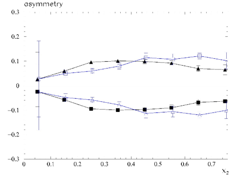
Figure 5: The asymmetry $(U-D)/(U+D)$ with positive ($U$) and negative ($D$) values of $\sin(\phi-\phi_{S_{2}})$ in Eq. (20) (see text), for Drell-Yan events from the Sivers effect in the $\pi^{\pm}p^{\uparrow}\to\mu^{+}\mu^{-}X$ reaction at $\sqrt{s}\sim 14$ GeV, $4<M<9$ GeV, and $1<q_{\scriptstyle T}<3$ GeV/$c$, using the parametrization of Eq. (22) for the Sivers function (see text). Triangles indicate $100\,000$ events collected in $x_{2}$ bins for the $\pi^{-}$ beam and with $N_{u}>0$; squares for $N_{u}<0$. Open triangles indicate $25\,000$ events for the $\pi^{+}$ beam and with $N_{u}>0$; open squares for $N_{u}<0$. Lines are drawn to guide the eye.

In Fig. 5, the asymmetry $(U-D)/(U+D)$ is shown for each bin $x_{2}$. Average asymmetries and (statistical) error bars are obtained, as usual, by 10 independent repetitions of the simulation. Boundary values of $x_{2}$ beyond 0.7 are excluded because of very low statistics. The triangles indicate the results with the $\pi^{-}$ beam obtained by Eq. (23) assuming that $f_{1\scriptstyle T}^{\perp}$ changes sign from SIDIS to Drell-Yan Collins (2002). For sake of comparison, the squares illustrate the opposite results that one would obtain by ignoring such prediction. Finally, the open triangles and open squares refer to the same situation, respectively, but for the $\pi^{+}$ beam.

In the valence picture of the $(\pi^{-})\pi^{+}-p$ collision where the $(\bar{u}u)\,\bar{d}d$ annihilation dominates, the SSA for the Drell-Yan process induced by $\pi^{+}$ has opposite sign with respect to $\pi^{-}$ because of the opposite signs for the normalization $N_{f},\,f=u,d$, in the parametrization (22). Apart for very low $x_{2}$ values where the parton picture leading to Eq. (1) becomes questionable, the error bars are very small and allow for a clean reconstruction of the asymmetry shape and, more importantly, for a conclusive test of the predicted sign change in $f_{1\scriptstyle T}^{\perp}$.

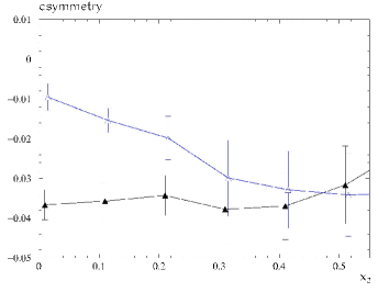
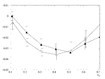
Figure 6: The asymmetry $(U-D)/(U+D)$ with positive ($U$) and negative ($D$) values of $\sin(\phi+\phi_{S_{2}})$ in Eq. (24) (see text), for $200\,000$ Drell-Yan events from the Boer-Mulders effect. In the left panel, the $\pi^{-}p^{\uparrow}\to\mu^{+}\mu^{-}X$ reaction is considered at $\sqrt{s}\sim 10$ GeV, $1.5<M<2.5$ GeV, and $1<q_{\scriptstyle T}<3$ GeV/$c$; triangles for $h_{1}(x_{2},\langle q\rangle/H_{2}^{\uparrow})/f_{1}(x_{2},\langle q\rangle/H_{2})=\sqrt{1-x_{2}}$ inside Eq. (27) (see text), open triangles for $h_{1}(x_{2},\langle q\rangle/H_{2}^{\uparrow})/f_{1}(x_{2},\langle q\rangle/H_{2})=\sqrt{x_{2}}$; the $\langle q\rangle$ notation represents a common average term that replaces each contribution in the flavor sum (for further details, see text). In the right panel, the $\bar{p}p^{\uparrow}\to\mu^{+}\mu^{-}X$ reaction is considered at $\sqrt{s}\sim 14$ GeV, $4<M<9$ GeV; triangles for the results from the spectator diquark model with $1<q_{\scriptstyle T}<3$ GeV/$c$, open triangles for $2<q_{\scriptstyle T}<3$ GeV/$c$. In all cases, the further cut $60^{\rm o}<\theta<120^{\rm o}$ is applied. Lines are drawn to guide the eye.

IV.3 The Boer-Mulders effect

For the Boer-Mulders effect, we have collected $200\,000$ Drell-Yan events for the $\pi^{-}p^{\uparrow}\to\mu^{+}\mu^{-}X$ reaction at the lower $\sqrt{s}\sim 10$ GeV in order to keep a significant statistics; the muon invariant mass is restricted in the $1.5<M<2.5$ GeV range, with $1<q_{\scriptstyle T}<3$ GeV/$c$ and $60^{\rm o}<\theta<120^{\rm o}$. In the left panel of Fig. 6, the asymmetry $(U-D)/(U+D)$ is shown for each bin $x_{2}$ between the events with positive $(U)$ and negative $(D)$ values of $\sin(\phi+\phi_{S_{2}})$ in Eq. (24). Triangles correspond to the choice $h_{1}(x_{2},\langle q\rangle/H_{2}^{\uparrow})/f_{1}(x_{2},\langle q\rangle/H_{2})=\sqrt{1-x_{2}}$ inside Eq. (27), open triangles to the choice $h_{1}(x_{2},\langle q\rangle/H_{2}^{\uparrow})/f_{1}(x_{2},\langle q\rangle/H_{2})=\sqrt{x_{2}}$ (see Sec. III.3). Both choices respect the Soffer bound between $h_{1}$ and $f_{1}$. The error bars are only statistical and are small because of the copious statistics. As it is evident in the figure, for $x_{2}<0.3$ it is possible to distinguish the trend of the triangles (which statistically reflects the descending trend of the input function $\sqrt{1-x_{2}}$) from the one of the open triangles (referred to the ascending $\sqrt{x_{2}}$). We made simulations also at the same kinematics of the previous Sivers effect, namely for $\sqrt{s}\sim 14$ GeV and for muon pair invariant masses in the $4<M<9$ GeV range. The statistical error bars remain small and the SSA is definitely nonvanishing, but a clear distinction between the two trends is no longer possible.

In the right panel of Fig. 6, the same $(U-D)/(U+D)$ asymmetry is considered for the $\bar{p}p^{\uparrow}\to\mu^{+}\mu^{-}X$ reaction at $\sqrt{s}\sim 14$ GeV with muon invariant mass in the $4<M<9$ GeV range and $60^{\rm o}<\theta<120^{\rm o}$. The same sample of $200\,000$ events is now produced by input parton densities from the spectator diquark model. Triangles correspond to the events with the cut $1<q_{\scriptstyle T}<3$ GeV/$c$, open triangles with $2<q_{\scriptstyle T}<3$ GeV/$c$. Again, boundary values of $x_{2}$ beyond 0.7 are excluded because of very low statistics. Within the (statistical) error bars, there is no sensitivity to the cut in the lepton pair transverse momentum.

The overall size of the spin asymmetry is small and the reached statistical accuracy indicates that the size of the sample is not responsible for this feature (see also Ref. Sissakian et al. (2005)). Rather, it is the outcome of a combination of several sources. First of all, the phenomenological ${\bm{p}}_{\scriptstyle T}$ dependence of $h_{1}^{\perp}$ in Eq. (16), which also affects the result with the spectator diquark model according to the approximation described in Sec. III.3: it is fixed to reproduce the data of Ref. Guanziroli et al. (1988), which indicate significant asymmetries only for very large ${\bm{p}}_{\scriptstyle T}$ beyond the range of interest here. Secondly, the target dilution factor: it is unavoidably introduced by the features of the actual target that effectively reproduces a transversely polarized proton; at COMPASS the wanted ”polarized” events are 1/4 of the total number of collisions on the $NH_{3}$ molecule. Finally, the Soffer bound: the various choices for the ratio $h_{1}(x_{2},\langle q\rangle/H_{2}^{\uparrow})/f_{1}(x_{2},\langle q\rangle/H_{2})$ on one side, as well as the expressions (18) and (28) for $f_{1},h_{1}^{\perp},$ and $h_{1}$ in the spectator diquark model on the other side, are tightly limited by this constraint.

V Two-hadron inclusive production in hadronic collisions

As anticipated in Sec. I, the most popular technique to extract the transversity $h_{1}$ is to measure a single-spin asymmetry (SSA) in SIDIS production of pions on transversely polarized proton targets. The parton fragmentation into the detected pion can be described by a quark-quark correlator similar to the one of Eq. (6), namely

$$\Delta(z,{\bm{k}}_{\scriptstyle T}) = \frac{1}{2z}\,\int dk^{+}\,\sum_{\scriptstyle X}\,\int\frac{d^{4}\xi}{(2\pi)^{4}}\,e^{ik\cdot\xi}\,\langle 0|U_{\left[\infty,\xi\right]}\,\psi(\xi)|P_{h},X\rangle\,\langle P_{h},X|\bar{\psi}(0)\,U_{\left[0,\infty\right]}|0\rangle\Big{|}_{k^{-}=P_{h}^{-}/z}$$ (29)

$$= \frac{1}{2P_{h}^{-}}\,\left\{D_{1}(z,{\bm{k}}_{\scriptstyle T})\,\kern 1.99997ptP\kern-5.0pt/_{h}+H_{1}^{\perp}(z,{\bm{k}}_{\scriptstyle T})\,\sigma_{\mu\nu}\,\frac{k^{\mu}P_{h}^{\nu}}{M_{h}}\right\}\;,$$

which holds, in general, for a transversely polarized parton with momentum $k$, fragmenting in an unpolarized hadron with momentum $P_{h}$ and mass $M_{h}$. Applying the same definition of projection as in Eq. (7), and following again the prescriptions of Ref. Bacchetta et al. (2004a), we can define the number density $D_{h/qs_{T}}$ of unpolarized hadrons $h$ in a parton with flavor $q$ and transverse polarization ${\bm{s}}_{\scriptstyle T}$:

$$D_{h/qs_{T}} = \frac{1}{2}\,\left(\Delta^{[\gamma_{\mu}\,n_{\scriptscriptstyle+}^{\mu}/2]}+\Delta^{[i\sigma_{\mu\nu}\,n_{\scriptscriptstyle+}^{\mu}s_{\scriptscriptstyle T}^{\nu}\gamma_{5}/2]}\right)$$ (30)

$$= \frac{1}{2}\,\left\{D_{1}^{q}(z,{\bm{k}}_{\scriptstyle T})+H_{1}^{\perp\,q}(z,{\bm{k}}_{\scriptstyle T})\,\frac{\hat{\bm{k}}\times{\bm{P}}_{h\scriptstyle T}\cdot{\bm{s}_{\scriptstyle T}}}{zM_{h}}\right\}\;,$$

where $n_{+}=(0,1,{\bm{0}}_{\scriptstyle T})$. It is evident that the unpolarized ”decay” function is given by the sum upon all possible polarizations of the fragmenting quark, namely $D_{1}^{q}=D_{h/q\uparrow}+D_{h/q\downarrow}$, while the Collins function is deduced by

$$D_{h/q\uparrow}-D_{h/q\downarrow}=H_{1}^{\perp\,q}(z,{\bm{k}}_{\scriptstyle T})\,\frac{\hat{\bm{k}}\times{\bm{P}}_{h\scriptstyle T}\cdot{\bm{s}_{\scriptstyle T}}}{zM_{h}}\;.$$ (31)

Combining the quark-quark correlators of Eq. (6) and (29), together with the elementary cross section for the virtual photon absorption, it is possible to build the leading-twist expression of the SIDIS cross section for a transversely polarized target in a factorized picture (for the general expression, see Ref. Bacchetta et al. (2007b)). The transversity $h_{1}$ can be extracted by the following SSA:

$$\frac{\displaystyle{\int d\phi_{\scriptstyle S}d{\bm{P}}_{h\scriptstyle T}\frac{|{\bm{P}}_{h\scriptstyle T}|}{M_{h}}\,\sin(\phi_{h}+\phi_{\scriptstyle S})\,(d\sigma^{\uparrow}-d\sigma^{\downarrow})}}{\displaystyle{\int d\phi_{\scriptstyle S}d{\bm{P}}_{h\scriptstyle T}\,(d\sigma^{\uparrow}+d\sigma^{\downarrow})}}\propto\frac{\sum_{q\bar{q}}\,e^{2}_{q}\,h_{1}^{q}(x)\,H_{1}^{\perp q\,(1)}(z)}{\sum_{q\bar{q}}\,e^{2}_{q}\,f_{1}^{q}(x)\,D_{1}^{q}(z)}\;,$$ (32)

where $\phi_{\scriptstyle S},\phi_{h},$ are the azimuthal orientations with respect to the scattering plane of the target polarization vector and of the hadronic plane containing ${\bm{P}}_{h\scriptstyle T}$, respectively. From Eq. (32) it is evident that this strategy, known as Collins effect Collins (1993), requires the knowledge of the entire ${\bm{P}}_{h\scriptstyle T}$ distribution of the produced hadron $h$, which is obviously not possible from the experimental point of view. But also theoretically there are some complications, since the factorization proof and the evolution equations of TMD parton density functions are more involved Collins and Metz (2004); Ji et al. (2005). For the case of hadronic collisions leading to semi-inclusive final states in specific kinematic conditions, very recently an explicit factorization-breaking mechanism has been discussed for a ${\bm{k}}_{\scriptstyle T}$-dependent elementary hard cross section Collins and Qiu (2007).

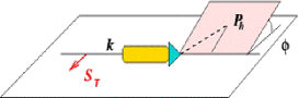
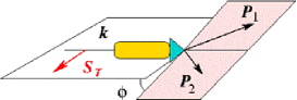
Figure 7: In the left panel, the graphic representation of the mixed product ${\bm{k}}\times{\bm{P}}_{h\scriptstyle T}\cdot{\bm{s}}_{\scriptstyle T}$, which governs the Collins effect. In the right panel, the mixed product ${\bm{P}}_{1}\times{\bm{P}}_{2}\cdot{\bm{s}}_{\scriptstyle T}$, which describes the asymmetric distribution in $\phi$ of a hadron pair collinear to the jet axis $\hat{\bm{k}}$.

In Fig. 7, the Collins effect produced by the mixed product ${\bm{k}}\times{\bm{P}}_{h\scriptstyle T}\cdot{\bm{s}}_{\scriptstyle T}$ (left panel), is compared with the more exclusive situation where two hadrons are produced Collins et al. (1994); Jaffe et al. (1998). In this case (right panel), it is possible to relate the polarization ${\bm{s}}_{\scriptstyle T}$ of the fragmenting quark to the azimuthal orientation of the plane containing the two hadrons via the mixed product ${\bm{P}}_{1}\times{\bm{P}}_{2}\cdot{\bm{s}}_{\scriptstyle T}$. If $P_{h}=P_{1}+P_{2}$ is the total momentum of the pair, and $2R=P_{1}-P_{2}$ the relative one, the asymmetry survives even if the pair is taken collinear to the fragmenting quark direction $\hat{\bm{k}}$, or alternatively if the dependence upon ${\bm{P}}_{h\scriptstyle T}$ is integrated away, contrary to what happens in the Collins effect. In fact, the quark-quark correlator for the fragmentation of a transversely polarized quark into two unpolarized hadrons reads

$$\Delta(z,\zeta,{\bm{k}}_{\scriptstyle T},{\bm{R}}_{\scriptstyle T}^{2},\phi_{\scriptstyle R}) = \frac{1}{8z\,(1-\zeta^{2})}\,\int dk^{+}\,\sum_{\scriptstyle X}\,\int\frac{d^{4}\xi}{(2\pi)^{4}}\,e^{+ik\cdot\xi}\langle 0|{\cal U}_{(-\infty,\xi)}\,\psi(\xi)|P_{h},R;X\rangle$$ (33)

$$\mbox{\hskip 170.71652pt}\times\,\langle P_{h},R;X|\bar{\psi}(0)\,{\cal U}_{(0,-\infty)}|0\rangle\,\Big{|}_{k^{-}=P_{h}^{-}/z}$$

$$= \frac{1}{16\pi}\left\{D_{1}(z,\zeta,{\bm{k}}_{\scriptstyle T},{\bm{R}}_{\scriptstyle T}^{2})+i\frac{\kern 1.99997ptR\kern-5.0pt/_{\scriptstyle T}}{M_{h}}\,H_{1}^{{<\kern-2.10002pt{\scriptscriptstyle)}}}(z,\zeta,{\bm{k}}_{\scriptstyle T},{\bm{R}}_{\scriptstyle T}^{2})\right.$$

$$\left.+i\frac{\kern 1.99997ptk\kern-4.49997pt/_{\scriptstyle T}}{M_{h}}\,H_{1}^{\perp}(z,\zeta,{\bm{k}}_{\scriptstyle T},{\bm{R}}_{\scriptstyle T}^{2})+\frac{\epsilon_{\scriptstyle T}^{ij}k_{\scriptstyle Ti}R_{\scriptstyle Tj}}{M_{h}^{2}}\gamma_{5}\,G_{1}^{\perp}(z,\zeta,{\bm{k}}_{\scriptstyle T},{\bm{R}}_{\scriptstyle T}^{2})\right\}\,\gamma^{+}\;,$$

where $z=P_{h}^{-}/k^{-}=z_{1}+z_{2}$ is the fraction of quark energy delivered to the pair, $\zeta=2R^{-}/P_{h}^{-}=(z_{1}-z_{2})/z$ describes how this fraction is split inside the pair, and $\epsilon_{\scriptstyle T}^{ij}\equiv\epsilon^{-+ij}$. The new fragmentation functions appearing in Eq. (33) are named Dihadron Fragmentation Functions (DiFF) Bianconi et al. (2000). The $H_{1}^{\perp}$ is the analogue of the Collins function, while $G_{1}^{\perp}$ describes the same situation but for the fragmenting quark longitudinally polarized (a sort of analogue of the jet handedness, see Ref. Boer et al. (2003) and references therein). After integrating upon ${\bm{k}}_{\scriptstyle T}=-{\bm{P}}_{h\scriptstyle T}/z$, both disappear and we are left with

$$\Delta(z,\zeta,{\bm{R}}_{\scriptstyle T}^{2},\phi_{\scriptstyle R})=\frac{1}{16\pi}\left\{D_{1}(z,\zeta,{\bm{R}}_{\scriptstyle T}^{2})+i\frac{\kern 1.99997ptR\kern-5.0pt/_{\scriptstyle T}}{M_{h}}\,H_{1}^{{<\kern-2.10002pt{\scriptscriptstyle)}}}(z,\zeta,{\bm{R}}_{\scriptstyle T}^{2})\right\}\,\gamma^{+}\;.$$ (34)

Apart for the usual ”decay” probability $D_{1}$, a potentially asymmetric term survives involving the chiral-odd DiFF $H_{1}^{{<\kern-2.10002pt{\scriptscriptstyle)}}}$, which appears as the natural partner of the transversity $h_{1}$ in the SSA Radici et al. (2002)

$$\frac{1}{\sin(\phi_{\scriptstyle R}+\phi_{\scriptstyle S})}\,\frac{d\sigma^{\uparrow}-d\sigma^{\downarrow}}{d\sigma^{\uparrow}+d\sigma^{\downarrow}}\propto\frac{|{\bm{R}}|}{M_{h}}\,\frac{\sum_{q\bar{q}}\,e_{q}^{2}\,h_{1}^{q}(x)\,H_{1}^{{<\kern-2.10002pt{\scriptscriptstyle)}}\,q}(z,\zeta,{\bm{R}}_{\scriptstyle T}^{2})}{\sum_{q\bar{q}}\,e_{q}^{2}\,f_{1}^{q}(x)\,D_{1}^{q}(z,\zeta,{\bm{R}}_{\scriptstyle T}^{2})}\;.$$ (35)

The $H_{1}^{<\kern-2.10002pt{\scriptscriptstyle)}}$ equally describes the fragmentation of a transversely polarized quark into two unpolarized hadrons as $H_{1}^{\perp}$, but it survives the ${\bm{k}}_{\scriptstyle T}$ integration since it is related to the asymmetry depicted in Fig. 7, which is connected to the ${\bm{R}}_{\scriptstyle T}$ vector. In this respect, any observable related to the asymmetry quantitatively described by $H_{1}^{{<\kern-2.10002pt{\scriptscriptstyle)}}}$ is free of the problems mentioned above about the Collins mechanism, in particular about the ${\bm{k}}_{\scriptstyle T}$ factorization.

It is possible also to expand these DiFF in the relative partial waves of the two hadrons, by suitably rewriting the $\zeta$ dependence in their c.m. frame Bacchetta and Radici (2003). Very recently, the HERMES collaboration reported measurements of the SSA in Eq. (35) involving only the interference between $s-$ and $p-$wave components, which is necessary to generate naïve T-odd functions like $H_{1}^{<\kern-2.10002pt{\scriptscriptstyle)}}$ van der Nat (2005). The COMPASS collaboration also presented analogous preliminary results Joosten (2005). In the meanwhile, the BELLE collaboration is planning to measure $H_{1}^{{<\kern-2.10002pt{\scriptscriptstyle)}}}$ in the near future Abe et al. (2006). A spectator model calculation of leading-twist DiFF has been built by tuning the parameters on the output of pion pair distributions (proportional to $D_{1}$) from PYTHIA, after adapting it to the HERMES kinematics Bacchetta and Radici (2006). Evolution equations for DiFF have been also studied, including the full dependence upon ${\bm{R}}_{\scriptstyle T}^{2}$, or, equivalently, upon the pair invariant mass Ceccopieri et al. (2007).

Here, we reconsider the proposal formulated for the first time in Ref. Bacchetta and Radici (2004), namely to use hadronic collisions on a transversely polarized proton target and inclusively detect one (or two) pairs of pions.

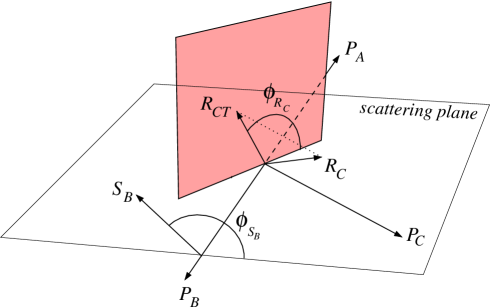
Figure 8: Description of the kinematics for the proton-proton annihilation into a single pair in a jet.

We consider first the process $A+B\rightarrow(h_{1}h_{2})_{C}+X$, where two protons (with momenta $P_{A},P_{B}$, and spin vectors $S_{A},S_{B}$) collide, and two unpolarized hadrons $h_{1},h_{2}$, with momenta $P_{1},P_{2}$, masses $M_{1},M_{2},$ and invariant mass squared $M_{C}^{2}=P_{C}^{2}=(P_{1}+P_{2})^{2}$, are inclusively detected inside the same jet. The intrinsic transverse component ${\bm{P}}_{C\scriptstyle T}$ with respect to the jet axis is integrated over and, consequently, ${\bm{P}}_{C}$ is taken parallel to the jet axis itself. The component ${\bm{P}}_{C\perp}$ perpendicular to the beam direction (defined by ${\bm{P}}_{A}$, see Fig. 8) serves as the hard scale of the process; it is assumed to be much bigger than the masses of the colliding hadrons and of $M_{h}$. The following analysis is valid only at leading order in $1/|{\bm{P}}_{C\perp}|$, i.e. at leading twist.

The azimuthal angles are defined in the hadronic center of mass as follows (see also Fig. 8)

$$\cos\phi_{S_{A}} =\frac{(\hat{\bm{P}}_{A}\times{\bm{P}}_{C})}{|\hat{\bm{P}}_{A}\times{\bm{P}}_{C}|}\cdot\frac{(\hat{\bm{P}}_{A}\times{\bm{S}}_{A})}{|\hat{\bm{P}}_{A}\times{\bm{S}}_{A}|}, \sin\phi_{S_{A}} =\frac{({\bm{P}}_{C}\times{\bm{S}}_{A})\cdot\hat{\bm{P}}_{A}}{|\hat{\bm{P}}_{A}\times{\bm{P}}_{C}|\,|\hat{\bm{P}}_{A}\times{\bm{S}}_{A}|},$$ (36)

$$\cos\phi_{S_{B}} =\frac{(\hat{\bm{P}}_{B}\times{\bm{P}}_{C})}{|\hat{\bm{P}}_{B}\times{\bm{P}}_{C}|}\cdot\frac{(\hat{\bm{P}}_{B}\times{\bm{S}}_{B})}{|\hat{\bm{P}}_{B}\times{\bm{S}}_{B}|}, \sin\phi_{S_{B}} =\frac{({\bm{P}}_{C}\times{\bm{S}}_{B})\cdot\hat{\bm{P}}_{B}}{|\hat{\bm{P}}_{B}\times{\bm{P}}_{C}|\,|\hat{\bm{P}}_{B}\times{\bm{S}}_{B}|},$$ (37)

$$\cos\phi_{R} =\frac{(\hat{\bm{P}}_{C}\times{\bm{P}}_{A})}{|\hat{\bm{P}}_{C}\times{\bm{P}}_{A}|}\cdot\frac{(\hat{\bm{P}}_{C}\times{\bm{R}}_{C})}{|\hat{\bm{P}}_{C}\times{\bm{R}}_{C}|}, \sin\phi_{R} =\frac{({\bm{P}}_{A}\times{\bm{R}}_{C})\cdot\hat{\bm{P}}_{C}}{|\hat{\bm{P}}_{C}\times{\bm{P}}_{A}|\,|\hat{\bm{P}}_{C}\times{\bm{R}}_{C}|}\;.$$ (38)

The partons involved in the elementary scattering have momenta $p_{a}=x_{a}P_{A}$, $p_{b}=x_{b}P_{B}$, and $p_{c}=P_{C}/z_{c}$. Also the usual Mandelstam variables have a counterpart at the elementary partonic level:

$$\hat{s} =x_{a}x_{b}\,s, \hat{t} =\frac{x_{a}}{z_{c}}\,t, \hat{u}=\frac{x_{b}}{z_{c}}\,u\;.$$ (39)

Conservation of momentum at the partonic level implies that

$$\begin{split}\hat{s}\,\delta(\hat{s}+\hat{t}+\hat{u})&=z_{c}\,\delta\left(z_{c}+\frac{x_{a}t+x_{b}u}{x_{a}x_{b}s}\right)\,\stackrel{{\scriptstyle\mbox{\tiny c.m.s.}}}{{=}}\,z_{c}\,\delta\left(z_{c}-\frac{|{\bm{P}}_{C\perp}|}{\sqrt{s}}\,\frac{x_{a}e^{-\eta_{C}}+x_{b}e^{\eta_{C}}}{x_{a}x_{b}}\right)\,\equiv\,z_{c}\,\delta\left(z_{c}-\bar{z}_{c}\right)\;,\end{split}$$ (40)

where $\eta_{C}$ is the pseudorapidity with respect to ${\bm{P}}_{A}$.

Therefore, the cross section can be written as

$$\begin{split}\frac{d\sigma}{d\eta_{C}\,d|{\bm{P}}_{C\perp}|\,d\zeta_{c}\,d{\bm{R}}_{C\scriptstyle T}\,d\phi_{S_{A}}\,d\phi_{S_{B}}}&=2\,|{\bm{P}}_{C\perp}|\sum_{a,b,c,d}\frac{1}{4}\sum_{({\rm all}\;\chi{\rm{}^{\prime}s})}\int\frac{dx_{a}dx_{b}}{4\pi^{2}z_{c}}\,\Phi_{a}(x_{a},S_{A})_{\chi_{a}^{\prime}\chi_{a}}\,\Phi_{b}(x_{b},S_{B})_{\chi_{b}^{\prime}\chi_{b}}\\ &\quad\frac{1}{16\pi\hat{s}^{2}}\,\hat{M}_{\chi_{c},\chi_{d};\chi_{a},\chi_{b}}\,\hat{M}^{\ast}_{\chi_{a}^{\prime},\chi_{b}^{\prime};\chi_{c}^{\prime}\chi_{d}^{\prime}}\,\Delta_{c}(\bar{z}_{c},\zeta_{c},{\bm{R}}_{C\scriptstyle T}^{2},\phi_{R_{C}})_{\chi_{c}^{\prime}\chi_{c}}\,\delta_{\chi_{d}^{\prime}\chi_{d}}\;,\end{split}$$ (41)

where the indices $\chi$’s refer to the chiralities/helicities of the partons, and the partonic hard amplitudes $\hat{M}(\hat{s},\hat{t},\hat{u})$ can be taken from Refs. Gastmans and Wu (1990); Bacchetta and Radici (2004). In Eq. (41), $\Phi$ and $\Delta$ are the same parton-parton correlators of Eqs. (6) and (33), after integrating upon the intrinsic tranverse momenta and using the parton helicity basis representation.

For initial quarks with flavor $a$ we have Jaffe and Ji (1992); Bacchetta et al. (2000)

$$\Phi_{a}(x_{a},S_{A})_{\chi_{a}^{\prime}\chi_{a}}=\left(\begin{array}[]{cc}f_{1}(x_{a})+S_{A\,L}\,g_{1}(x_{a})&|{\bm{S}}_{A\scriptstyle T}|\,e^{-i\phi_{S_{A}}}\,h_{1}(x_{a})\\[5.0pt] |{\bm{S}}_{A\scriptstyle T}|\,e^{i\phi_{S_{A}}}\,h_{1}(x_{a})&f_{1}(x_{a})-S_{A\,L}\,g_{1}(x_{a})\end{array}\right)\;.$$ (42)

The correlator is written in the helicity basis where ${\bm{P}}_{A}$ defines the $\hat{z}$ axis, with $S_{A\,L}$ and $|{\bm{S}}_{A\scriptstyle T}|$ indicating the parallel and transverse components of the polarization ${\bm{S}}_{A}$ with respect to ${\bm{P}}_{A}$, and the $\hat{x}$ axis is oriented along ${\bm{P}}_{C\perp}$. Similarly for quark $b$ in the hadron $B$. When the initial partons are gluons, in a spin-$\textstyle{\frac{1}{2}}$ target the $\Phi$ is diagonal because of angular momentum conservation Jaffe and Saito (1996); Mulders and Rodrigues (2001).

If the final fragmenting parton $c$ is a quark, we have

$$\Delta_{c}(z_{c},\zeta_{c},{\bm{R}}_{C\scriptstyle T}^{2},\phi_{R_{C}})_{\chi_{c}^{\prime}\chi_{c}}=\frac{1}{4\pi}\,\left(\begin{array}[]{cc}D_{1}&ie^{i\phi_{R_{C}}}\,\frac{|{\bm{R}}_{C\scriptstyle T}|}{M_{C}}\,H_{1}^{{<\kern-2.10002pt{\scriptscriptstyle)}}}\\[5.0pt] -ie^{-i\phi_{R_{C}}}\,\frac{|{\bm{R}}_{C\scriptstyle T}|}{M_{C}}\,H_{1}^{{<\kern-2.10002pt{\scriptscriptstyle)}}}&D_{1}^{q}\end{array}\right)\;,$$ (43)

where the helicity basis is now choosen with the $\hat{z}$ axis along ${\bm{P}}_{C}$ and the $\hat{x}$ axis along the component of ${\bm{P}}_{A}$ orthogonal to ${\bm{P}}_{C}$ (see Fig. 8). For final fragmenting gluons, because of angular momentum conservation the $\Delta_{c}$ can be obtained in analogy to the case of gluon distributions in spin-1 targets Jaffe and Manohar (1989):

$$\Delta_{c=g}(z_{c},\zeta_{c},{\bm{R}}_{C\scriptstyle T}^{2},\phi_{R_{C}})_{\chi_{c}^{\prime}\chi_{c}}=\frac{1}{4\pi}\,\left(\begin{array}[]{cc}\hat{G}&ie^{2i\phi_{R_{C}}}\,\frac{|{\bm{R}}_{C\scriptstyle T}|^{2}}{M_{C}^{2}}\,\delta\hat{G}^{<\kern-2.10002pt{\scriptscriptstyle)}}\\[5.0pt] -ie^{-2i\phi_{R_{C}}}\,\frac{|{\bm{R}}_{C\scriptstyle T}|^{2}}{M_{C}^{2}}\,\delta\hat{G}^{<\kern-2.10002pt{\scriptscriptstyle)}}&\hat{G}\end{array}\right)\;.$$ (44)

The functions $\hat{G}$ and $\delta\hat{G}^{<\kern-2.10002pt{\scriptscriptstyle)}}$ describe the decay into two unpolarized hadrons of an unpolarized and a transversely polarized gluon, respectively, where by ”transverse polarization” we mean linear polarization along two independent directions transverse to $\hat{z}$, as in the quark case Bacchetta and Radici (2004). Unfortunately, $\delta\hat{G}^{<\kern-2.10002pt{\scriptscriptstyle)}}$ cannot appear in connection with the quark transversity $h_{1}$ because of the mismatch in the units of helicity flip between a spin-$\textstyle{\frac{1}{2}}$ and a spin-1 objects, leading to the $\exp(i\phi_{R_{C}})$ and $\exp(2i\phi_{R_{C}})$ dependences in Eq. (42) and Eq. (44), respectively. It can be coupled to the gluon transversity $\delta G$, but only in a target with spin greater than $\textstyle{\frac{1}{2}}$ Jaffe and Manohar (1989).

When considering the process $pp^{\uparrow}\to(h_{1}h_{2})X$, the most interesting SSA is

$$A_{N}(\eta_{C},|{\bm{P}}_{C\perp}|,\zeta_{c},{\bm{R}}_{C\scriptstyle T}^{2},\phi_{R_{C}},\phi_{S_{B}})=\frac{d\sigma^{\uparrow}-d\sigma^{\downarrow}}{d\sigma^{\uparrow}+d\sigma^{\downarrow}}\equiv\frac{d\sigma_{UT}}{d\sigma_{UU}}\;,$$ (45)

where

$$d\sigma_{UU} = 2\,|{\bm{P}}_{C\perp}|\,\sum_{a,b,c,d}\int\frac{dx_{a}dx_{b}}{8\pi^{2}z_{c}}\,f_{1}^{a}(x_{a})\,f_{1}^{b}(x_{b})\,\frac{d\hat{\sigma}_{ab\to cd}}{d\hat{t}}\,D_{1}(\bar{z}_{c},\zeta_{c},{\bm{R}}_{C\scriptstyle T}^{2})\;,$$

$$d\sigma_{UT} = 2\,|{\bm{P}}_{C\perp}|\,\sum_{a,b,c,d}\,|{\bm{S}}_{B\scriptstyle T}|\,\sin{(\phi_{S_{B}}-\phi_{R_{C}})}\int\frac{dx_{a}dx_{b}}{8\pi^{2}z_{c}}\,f_{1}^{a}(x_{a})\,h_{1}^{b}(x_{b})\,\frac{d\Delta\hat{\sigma}_{ab^{\uparrow}\to c^{\uparrow}d}}{d\hat{t}}\,\frac{|{\bm{R}}_{C\scriptstyle T}|}{M_{C}}\,H_{1}^{{<\kern-2.10002pt{\scriptscriptstyle)}}}(\bar{z}_{c},\zeta_{c},{\bm{R}}_{C\scriptstyle T}^{2})\;.$$ (46)

Here, it is understood that when the parton is a gluon, we need to replace $f_{1}$ and $g_{1}$ with the momentum and helicity gluon distributions, respectively, as well as to have $D_{1}\to\hat{G}$. The elementary cross sections are Bacchetta and Radici (2004)

$$\frac{\hat{\sigma}_{ab\to cd}}{d\hat{t}} \equiv \frac{1}{16\pi\hat{s}^{2}}\,\frac{1}{4}\sum_{({\rm all}\;\chi{\rm{}^{\prime}s})}\,\hat{M}_{\chi_{c},\chi_{d};\chi_{a},\chi_{b}}\,\hat{M}^{\ast}_{\chi_{a},\chi_{b};\chi_{c}\chi_{d}}\;,$$

$$\frac{d\Delta\hat{\sigma}_{ab^{\uparrow}\to c^{\uparrow}d}}{d\hat{t}} \equiv \frac{1}{16\pi\hat{s}^{2}}\,\frac{1}{4}\sum_{({\rm all}\;\chi{\rm{}^{\prime}s})}\,\hat{M}_{\chi_{c},\chi_{d};\chi_{a},\chi_{b}}\,\hat{M}^{\ast}_{\chi_{a},-\chi_{b};-\chi_{c},\chi_{d}}\;.$$ (47)

In the polarized case, a parton $b$ is transversely polarized in a direction forming an azimuthal angle $\phi_{S_{b}}$ around ${\bm{P}}_{B}$ and the transverse polarization of parton $c$ forms the same azimuthal angle $\phi_{S_{c}}=\phi_{S_{b}}$ around ${\bm{P}}_{C}$ ($\phi_{S_{b}}$ and $\phi_{S_{c}}$ are defined analogously to $\phi_{S_{B}}$ and $\phi_{R_{C}}$, respectively, see Fig. 8).

Using Eq. (45), the extraction of $h_{1}$ is possible either by using models for DiFF Bacchetta and Radici (2006), or by awaiting for $e^{+}e^{-}$ measurements to determine DiFF at BELLE Grosse Perdekamp (2002), in combination with the recent one in SIDIS at HERMES van der Nat (2005). Experimental results at different energies can be presently related through DGLAP equations at NLL accuracy including full dependence upon ${\bm{R}}_{\scriptstyle T}^{2}$ Ceccopieri et al. (2007). However, DiFF can be measured independently in the very same proton-proton collisions analyzed so far, by simply detecting another hadron pair in the other recoiling back-to-back jet. In fact, by generalizing the formalism of Eqs. (41) and (46), we have Bacchetta and Radici (2004)

$$d\sigma_{UU}={\cal{A}}+\cos{(\phi_{R_{C}}-\phi_{R_{D}})}\;{\cal{B}}+\cos{(2\phi_{R_{C}}-2\phi_{R_{D}})}\;{\cal{C}}\;,$$ (48)

where

$${\cal{A}} = \sum_{a,b,c,d}\int\frac{dx_{a}}{8\pi^{2}}\,f_{1}^{a}(x_{a})\,\bar{x}_{b}\,f_{1}^{b}(\bar{x}_{b})\,\frac{d\hat{\sigma}_{ab\to cd}}{d\hat{t}}\,D_{1}(\bar{z}_{c},\zeta_{c},{\bm{R}}_{C\scriptstyle T}^{2})\,D_{1}(\bar{z}_{d},\zeta_{d},{\bm{R}}_{D\scriptstyle T}^{2})\;,$$

$${\cal{B}} = \sum_{a,b,c,d}\int\frac{dx_{a}}{8\pi^{2}}\,f_{1}^{a}(x_{a})\,\bar{x}_{b}\,f_{1}^{b}(\bar{x}_{b})\,\frac{d\Delta\hat{\sigma}_{ab\to c^{\uparrow}d^{\uparrow}}}{d\hat{t}}\,\frac{|{\bm{R}}_{C\scriptstyle T}|}{M_{C}}\,H_{1}^{{<\kern-2.10002pt{\scriptscriptstyle)}}}(\bar{z}_{c},\zeta_{c},{\bm{R}}_{C\scriptstyle T}^{2})\,\frac{|{\bm{R}}_{D\scriptstyle T}|}{M_{D}}\,H_{1}^{{<\kern-2.10002pt{\scriptscriptstyle)}}}(\bar{z}_{d},\zeta_{d},{\bm{R}}_{D\scriptstyle T}^{2})\;,$$

$${\cal{C}} = \sum_{a,b,c,d}\int\frac{dx_{a}}{8\pi^{2}}\,f_{1}^{a}(x_{a})\,\bar{x}_{b}\,f_{1}^{b}(\bar{x}_{b})\,\frac{d\Delta\hat{\sigma}_{ab\to c^{\uparrow}d^{\uparrow}}}{d\hat{t}}\,\frac{|{\bm{R}}_{C\scriptstyle T}|^{2}}{M_{C}^{2}}\,\delta\hat{G}^{{<\kern-2.10002pt{\scriptscriptstyle)}}}(\bar{z}_{c},\zeta_{c},{\bm{R}}_{C\scriptstyle T}^{2})\,\frac{|{\bm{R}}_{D\scriptstyle T}|^{2}}{M_{D}^{2}}\,\delta\hat{G}^{{<\kern-2.10002pt{\scriptscriptstyle)}}}(\bar{z}_{d},\zeta_{d},{\bm{R}}_{D\scriptstyle T}^{2})\;,$$ (49)

and

$$\frac{d\Delta\hat{\sigma}_{ab\to c^{\uparrow}d^{\uparrow}}}{d\hat{t}}\equiv\frac{1}{16\pi\hat{s}^{2}}\,\frac{1}{4}\sum_{({\rm all}\;\chi{\rm{}^{\prime}s})}\,\hat{M}_{\chi_{c},\chi_{d};\chi_{a},\chi_{b}}\,\hat{M}^{\ast}_{\chi_{a},\chi_{b};-\chi_{c},-\chi_{d}}\;,$$ (50)

with $\bar{x}_{b}=x_{a}\,e^{-\eta_{C}}\,e^{-\eta_{D}}$ by momentum conservation.

All functions ${\cal A},{\cal B}$ and ${\cal C}$ are interesting. The first two contain pairs of the DiFF $D_{1},H_{1}^{{<\kern-2.10002pt{\scriptscriptstyle)}}}$, one for each hadron pair: measuring the symmetric and the $\cos{(\phi_{R_{C}}-\phi_{R_{D}})}$ asymmetric parts of the cross section for the $pp\to(h_{1}h_{2})_{jet_{C}}(h_{1}h_{2})_{jet_{D}}X$ process, it allows the extraction of $D_{1}$ and $H_{1}^{{<\kern-2.10002pt{\scriptscriptstyle)}}}$ and, in turn, of the transversity $h_{1}$ from the asymmetry $A_{N}$ of Eqs. (45,46) in the corresponding polarized collision $pp^{\uparrow}\to(h_{1}h_{2})X$. Finally, the ${\cal C}$ observable describes the fragmentation of two transversely (linearly) polarized gluons into two transversely (linearly) polarized spin-1 resonances, which would not be available in a SIDIS process using spin-$\textstyle{\frac{1}{2}}$ proton targets.

VI Conclusions

Using energetic hadronic (pion) beams on a transversely polarized $NH_{3}$ target, it opens a new window at COMPASS for the exploration of the partonic (spin) structure of the nucleon. When releasing the condition for collinear elementary annihilations, the leading-twist cross section for the production of Drell-Yan muon pairs contains several azimuthal asymmetric terms, whose combined study would shed light on yet unresolved puzzles. For example, the $\cos 2\phi$ term in the unpolarized cross section involves twice the exotic partonic density $h_{1}^{\perp}$, the socalled Boer-Mulders function, that describes the unbalance in the distribution of tranversely polarized partons inside unpolarized spin-$\textstyle{\frac{1}{2}}$ hadrons. It could give a natural explanation of the role of this contribution in the yet unexplained violation of the socalled Lam-Tung sum rule. The same $h_{1}^{\perp}$ happens in the $\sin(\phi+\phi_{{}_{S}})$ asymmetric part of the polarized cross section, with $\phi_{{}_{S}}$ the target polarization orientation. It is convoluted with the tranversity $h_{1}$, then offering an alternative strategy for its extraction with respect to the standard Collins effect in SIDIS. Finally, the polarized cross section contains also a $\sin(\phi-\phi_{{}_{S}})$ asymmetric part where the usual momentum density $f_{1}$ is convoluted with $f_{1\scriptstyle T}^{\perp}$, the Sivers function, that describes the distortion of unpolarized parton distributions by the transverse polarization of the parent hadron. Studying all these partonic densities allows to build a 3-dim. map of partons inside hadrons via the determination of their angular orbital momentum, contributing to the solution of the yet pending puzzle about the spin sum rule of the proton. Moreover, a theorem based on very general hypotheses, would predict a sign change for $f_{1\scriptstyle T}^{\perp}$ and $h_{1}^{\perp}$ being extracted from Drell-Yan measurements with respect to a SIDIS one. An experimental verification of this represents a formidable test of QCD in its nonperturbative domain.

Monte Carlo simulations of the above azimuthal (spin) asymmetries at COMPASS, reveal that a very good statistics can be reached in short running time, given the relative abundance of energetic pions in the beam and the foreseen high luminosity. As a consequence, COMPASS is an ideal place for studying the $\sin(\phi-\phi_{{}_{S}})$ single-spin asymmetry involving the Sivers function, and for testing its predicted sign change with respect to SIDIS. Very small statistical error bars are reachable also for the other two asymmetries, but experimental constraints coming from older experiments (NA10, E615,..) reduce the size of the simulated asymmetry; a lack of parametrizations for the Boer-Mulders function, either for proton targets or for pion beams, further makes its extraction an issue under debate.

We have also shown that in semi-inclusive (transversely polarized) collisions with production of one hadron pair in the same jet, it is possible to isolate the convolution $f_{1}\otimes h_{1}\otimes H_{1}^{{<\kern-2.10002pt{\scriptscriptstyle)}}}$, involving the $H_{1}^{<\kern-2.10002pt{\scriptscriptstyle)}}$ describing the fragmentation of a transversely polarized parton in the two observed hadrons, through the measurement of the asymmetry of the cross section in the azimuthal orientation of the pair around its c.m. momentum. In the production of two hadron pairs in two separate jets in unpolarized collisions, it is possible to isolate the convolution $f_{1}\otimes f_{1}\otimes H_{1}^{{<\kern-2.10002pt{\scriptscriptstyle)}}}\otimes H_{1}^{{<\kern-2.10002pt{\scriptscriptstyle)}}}$, through the measurement of the asymmetry of the cross section in the relative azimuthal orientation of the two pairs. Since no distribution and fragmentation functions with an explicit transverse-momentum dependence are required, there is no need to consider suppressed contributions in the elementary cross sections included in the convolutions and the discussed asymmetries remain at leading-twist. Therefore, contrary to what happens in SIDIS, proton-proton collisions offer a unique possibility to determine self-consistently all the unknown parton densities that are necessary to extract the transversity $h_{1}$. We believe that this option should be seriously considered at COMPASS.

References

- Airapetian et al. (2005) A. Airapetian et al. (HERMES), Phys. Rev. Lett. 94, 012002 (2005), eprint hep-ex/0408013.
- Diefenthaler (2005) M. Diefenthaler (2005), proceedings of the 13th International Workshop on Deep-Inelastic Scattering (DIS05), 27 Apr - 1 May, 2005, Madison - Wisconsin, eprint hep-ex/0507013.
- Avakian et al. (2005) H. Avakian, P. Bosted, V. Burkert, and L. Elouadrhiri (CLAS) (2005), proceedings of 13th International Workshop on Deep-Inelastic Scattering (DIS 05), 27 Apr - 1 May, 2005, Madison - Wisconsin, eprint nucl-ex/0509032.
- Alexakhin et al. (2005) V. Y. Alexakhin et al. (COMPASS), Phys. Rev. Lett. 94, 202002 (2005), eprint hep-ex/0503002.
- Radici and van der Steenhoven (2004) M. Radici and G. van der Steenhoven, CERN Courier 44, 51 (2004).
- Bunce et al. (1976) G. Bunce et al., Phys. Rev. Lett. 36, 1113 (1976).
- Adams et al. (1991) D. L. Adams et al. (FNAL-E704), Phys. Lett. B264, 462 (1991).
- Kane et al. (1978) G. L. Kane, J. Pumplin, and W. Repko, Phys. Rev. Lett. 41, 1689 (1978).
- Falciano et al. (1986) S. Falciano et al. (NA10), Z. Phys. C31, 513 (1986).
- Guanziroli et al. (1988) M. Guanziroli et al. (NA10), Z. Phys. C37, 545 (1988).
- Conway et al. (1989) J. S. Conway et al., Phys. Rev. D39, 92 (1989).
- Anassontzis et al. (1988) E. Anassontzis et al., Phys. Rev. D38, 1377 (1988).
- Lam and Tung (1980) C. S. Lam and W.-K. Tung, Phys. Rev. D21, 2712 (1980).
- Brandenburg et al. (1994) A. Brandenburg, S. J. Brodsky, V. V. Khoze, and D. Muller, Phys. Rev. Lett. 73, 939 (1994), eprint hep-ph/9403361.
- Eskola et al. (1994) K. J. Eskola, P. Hoyer, M. Vanttinen, and R. Vogt, Phys. Lett. B333, 526 (1994), eprint hep-ph/9404322.
- Berger and Brodsky (1979) E. L. Berger and S. J. Brodsky, Phys. Rev. Lett. 42, 940 (1979).
- Sivers (1990) D. W. Sivers, Phys. Rev. D41, 83 (1990).
- Collins (1993) J. C. Collins, Nucl. Phys. B396, 161 (1993), eprint [http://arXiv.org/abs]hep-ph/9208213.
- Collins and Qiu (2007) J. Collins and J.-W. Qiu, Phys. Rev. D 75, 114014 (2007), eprint arXiv:0705.2141 [hep-ph].
- Ji et al. (2005) X.-d. Ji, J.-p. Ma, and F. Yuan, Phys. Rev. D71, 034005 (2005), eprint hep-ph/0404183.
- Collins and Metz (2004) J. C. Collins and A. Metz, Phys. Rev. Lett. 93, 252001 (2004), eprint hep-ph/0408249.
- Boer and Mulders (1998) D. Boer and P. J. Mulders, Phys. Rev. D57, 5780 (1998), eprint [http://arXiv.org/abs]hep-ph/9711485.
- Boer (1999) D. Boer, Phys. Rev. D60, 014012 (1999), eprint hep-ph/9902255.
- Bacchetta et al. (2004a) A. Bacchetta, U. D’Alesio, M. Diehl, and C. A. Miller, Phys. Rev. D70, 117504 (2004a), eprint hep-ph/0410050.
- Bianconi and Radici (2005a) A. Bianconi and M. Radici, Phys. Rev. D71, 074014 (2005a), eprint hep-ph/0412368.
- Bianconi and Radici (2005b) A. Bianconi and M. Radici, J. Phys. G31, 645 (2005b), eprint hep-ph/0501055.
- Burkardt and Hwang (2004) M. Burkardt and D. S. Hwang, Phys. Rev. D69, 074032 (2004), eprint hep-ph/0309072.
- Collins (2002) J. C. Collins, Phys. Lett. B536, 43 (2002), eprint hep-ph/0204004.
- Aoki et al. (1997) S. Aoki, M. Doui, T. Hatsuda, and Y. Kuramashi, Phys. Rev. D56, 433 (1997), eprint hep-lat/9608115.
- Gockeler et al. (2006) M. Gockeler et al. (QCDSF) (2006), eprint hep-lat/0612032.
- Bianconi and Radici (2005c) A. Bianconi and M. Radici, Phys. Rev. D72, 074013 (2005c), eprint hep-ph/0504261.
- Bianconi and Radici (2006a) A. Bianconi and M. Radici, Phys. Rev. D73, 034018 (2006a), eprint hep-ph/0512091.
- Bianconi and Radici (2006b) A. Bianconi and M. Radici, Phys. Rev. D73, 114002 (2006b), eprint hep-ph/0602103.
- Collins et al. (1994) J. C. Collins, S. F. Heppelmann, and G. A. Ladinsky, Nucl. Phys. B420, 565 (1994), eprint [http://arXiv.org/abs]hep-ph/9305309.
- Jaffe et al. (1998) R. L. Jaffe, X. Jin, and J. Tang, Phys. Rev. Lett. 80, 1166 (1998), eprint [http://arXiv.org/abs]hep-ph/9709322.
- Radici et al. (2002) M. Radici, R. Jakob, and A. Bianconi, Phys. Rev. D65, 074031 (2002), eprint [http://arXiv.org/abs]hep-ph/0110252.
- van der Nat (2005) P. B. van der Nat (HERMES) (2005), eprint hep-ex/0512019.
- Joosten (2005) R. Joosten (HERMES) (2005), proceedings of the 13th International Workshop on Deep Inelastic Scattering (DIS 2005), Madison, Wisconsin, U.S.A., 27 Apr - 1 May 2005.
- Abe et al. (2006) K. Abe et al. (Belle), Phys. Rev. Lett. 96, 232002 (2006), eprint hep-ex/0507063.
- Bacchetta and Radici (2006) A. Bacchetta and M. Radici, Phys. Rev. D74, 114007 (2006), eprint hep-ph/0608037.
- Ceccopieri et al. (2007) F. A. Ceccopieri, M. Radici, and A. Bacchetta, Phys. Lett. B650, 81 (2007), eprint hep-ph/0703265.
- Bacchetta and Radici (2004) A. Bacchetta and M. Radici, Phys. Rev. D70, 094032 (2004), eprint hep-ph/0409174.
- Collins et al. (1985) J. C. Collins, D. E. Soper, and G. Sterman, Nucl. Phys. B250, 199 (1985), see also A. Efremov and A. Radyushkin, Theor. Math. Phys. 44, 664 (1981) [ Teor. Mat. Fiz. 44, 157 (1980)].
- Collins and Soper (1977) J. C. Collins and D. E. Soper, Phys. Rev. D16, 2219 (1977).
- Bomhof et al. (2004) C. J. Bomhof, P. J. Mulders, and F. Pijlman, Phys. Lett. B596, 277 (2004), eprint hep-ph/0406099.
- Altarelli et al. (1979) G. Altarelli, R. K. Ellis, and G. Martinelli, Nucl. Phys. B157, 461 (1979).
- Martin et al. (1998) O. Martin, A. Schafer, M. Stratmann, and W. Vogelsang, Phys. Rev. D57, 3084 (1998), eprint hep-ph/9710300.
- Kawamura et al. (2007) H. Kawamura, J. Kodaira, and K. Tanaka (2007), eprint hep-ph/0703079.
- Jakob et al. (1997) R. Jakob, P. J. Mulders, and J. Rodrigues, Nucl. Phys. A626, 937 (1997), eprint [http://arXiv.org/abs]hep-ph/9704335.
- Brodsky et al. (2002) S. J. Brodsky, D. S. Hwang, and I. Schmidt, Nucl. Phys. B642, 344 (2002), eprint hep-ph/0206259.
- Gamberg et al. (2007) L. P. Gamberg, G. R. Goldstein, and M. Schlegel (2007), eprint private communication.
- Bacchetta et al. (2004b) A. Bacchetta, A. Schaefer, and J.-J. Yang, Phys. Lett. B578, 109 (2004b), eprint hep-ph/0309246.
- Bacchetta et al. (2007a) A. Bacchetta, F. Conti, and M. Radici (2007a), eprint in preparation.
- Miyama and Kumano (1996) M. Miyama and S. Kumano, Comput. Phys. Commun. 94, 185 (1996), eprint hep-ph/9508246.
- Hirai et al. (1998) M. Hirai, S. Kumano, and M. Miyama, Comput. Phys. Commun. 111, 150 (1998), eprint hep-ph/9712410.
- Vogelsang and Yuan (2005) W. Vogelsang and F. Yuan, Phys. Rev. D72, 054028 (2005), eprint hep-ph/0507266.
- Adler et al. (2005) S. S. Adler et al. (PHENIX), Phys. Rev. Lett. 95, 202001 (2005), eprint hep-ex/0507073.
- Bianconi and Radici (2007) A. Bianconi and M. Radici, J. Phys. G 34, 1595 (2007), eprint hep-ph/0610317.
- Sissakian et al. (2005) A. Sissakian, O. Shevchenko, A. Nagaytsev, O. Denisov, and O. Ivanov (2005), eprint hep-ph/0512095.
- Bacchetta et al. (2007b) A. Bacchetta et al., JHEP 02, 093 (2007b), eprint hep-ph/0611265.
- Bianconi et al. (2000) A. Bianconi, S. Boffi, R. Jakob, and M. Radici, Phys. Rev. D62, 034008 (2000), eprint [http://arXiv.org/abs]hep-ph/9907475.
- Boer et al. (2003) D. Boer, R. Jakob, and M. Radici, Phys. Rev. D67, 094003 (2003), eprint hep-ph/0302232.
- Bacchetta and Radici (2003) A. Bacchetta and M. Radici, Phys. Rev. D67, 094002 (2003), eprint hep-ph/0212300.
- Gastmans and Wu (1990) R. Gastmans and T. T. Wu, The Ubiquitous photon: Helicity method for QED and QCD, International series of monographs on physics (Clarendon, Oxford, UK, 1990).
- Jaffe and Ji (1992) R. L. Jaffe and X. Ji, Nucl. Phys. B375, 527 (1992).
- Bacchetta et al. (2000) A. Bacchetta, M. Boglione, A. Henneman, and P. J. Mulders, Phys. Rev. Lett. 85, 712 (2000), eprint [http://arXiv.org/abs]hep-ph/9912490.
- Jaffe and Saito (1996) R. L. Jaffe and N. Saito, Phys. Lett. B382, 165 (1996), eprint hep-ph/9604220.
- Mulders and Rodrigues (2001) P. J. Mulders and J. Rodrigues, Phys. Rev. D63, 094021 (2001), eprint hep-ph/0009343.
- Jaffe and Manohar (1989) R. L. Jaffe and A. Manohar, Phys. Lett. B223, 218 (1989).
- Grosse Perdekamp (2002) M. Grosse Perdekamp, Nucl. Phys. Proc. Suppl. 105, 71 (2002).