Lateral distribution and the energy determination of showers along the ankle

Abstract

The normalization constant of the lateral distribution function (LDF) of an extensive air shower is a monotonous (almost linear) increasing function of the energy of the primary. Therefore, the interpolated signal at some fixed distance from the core can be calibrated to estimate the energy of the shower. There is, somehow surprisingly, a reconstructed optimal distance, $r_{opt}$, at which the effects on the inferred signal, $S(r_{opt})$, of the uncertainties on true core location, LDF functional form and shower-to-shower fluctuations are minimized. We calculate the value of $r_{opt}$ as a function of surface detector separation, energy and zenith angle and we demonstrate the advantage of using the $r_{opt}$ value of each individual shower instead of a same fixed distance for every shower, specially in dealing with events with saturated stations. The effects on the determined spectrum are also shown.

1 Introduction

In order to determine the energy of cosmic rays with surface detectors arrays, first the lateral distribution function (LDF) of the shower particles, i.e. the particles density or signal versus distance to shower core location, is fitted assuming a known functional form. Following Hillas [1] proposal, the signal at some fixed distance of the shower core $S(r_{opt})$ for all the showers, independent of their energy or direction, is used to relate it with primary energy, usually using monte carlo simulations. The optimum distance $r_{opt}$ is mainly related to the geometry of the array.

We show that this method may not reconstruct properly the shape of the spectrum. We use an AGASA-like experiment [2] as case study and inject both a single power law and a simplified, yet realistic, structured spectrum above $10^{17.7}$ eV. A special analysis has been done for saturated events.

2 Method

A previous version of our algorithm was presented in [3]. We use a simplified numerical approach to the simulation of extensive air shower detection in a surface array. Our ideal detector is an infinite array of equally spaced stations distributed in elementary triangular cells of 1 km side.

The input spectrum is a perfect power law spectrum with index -3.0 from $10^{18.0}$ to $10^{20.1}$ and with an isotropic zenith distribution from 0 to 45 degrees. The number of events is 230.000, approximately the same statistic as the spectrum reported by AGASA. In a second case, we used a structured spectrum (with second knee, ankle and GZK-cut-off, and exposure-limited at low energy) from $10^{17.7}$ to $10^{21.0}$ eV as input.

Firstly, we select random core position inside an elementary cell, and the signal of each station is estimated using the LDF reported by Auger [4]:

$$S(r_{km},E_{EeV},\theta)=\frac{7.53\;E^{0.95}\;2^{\beta(\theta)}}{\sqrt{1+11.8[sec(\theta)-1]^{2}}}$$

$$\times r^{-\beta(\theta)}\times(1+r)^{-\beta(\theta)}$$ (1)

where $\beta(\theta)=3.1-0.7sec(\theta)$. The signal expected at each station is then fluctuated by Poissonian noise and recorded if it is above a threshold of 3.0 VEM (Vertical Equivalent Muons, the signal deposited by one vertical muon in an Auger water Cerenkov tank). Stations with a signal $S_{i}>S(0.2$ km $,1$ EeV $,0^{o})$ are considered saturated and are excluded.

The real core position is now moved using a gaussian distribution centered at this point. The sigma of this distribution is set taking into account the uncertainty in core determination, which depends on the array geometry and primary energy [5]. The new core position simulates the reconstructed core. In order to mimic the reconstruction procedure we fit the signals of the triggered stations with the LDF of the AGASA form:

$$\log S(r_{m})=a_{1}-a_{2}\log(r/r_{M})-0.6\log(1+r^{2})$$ (2)

with $r_{M}=91.6$ m, the moliere radius at AGASA altitude. Finally, the signal at 600 m ($S_{\theta}(600)$), is used to estimate the primary energy.

For the same shower, another procedure is done to obtained its real optimum distance $r_{opt}$. The reconstructed core is shifted 50 times using again a gaussian distribution centered at this point and with the same sigma as before. For each new core position, an LDF is fitted and the point $r_{opt}$ is defined as the location of the minimum dispersion. With the signal at this point $S(r_{opt})$, the energy of the primary is again estimated.

2.1 Conversion between Auger and AGASA LDFs

A conversion of units between the LDF from Auger (that we have used to assign the signal in each station) and the LDF from AGASA (that we will use for energy determination) is needed. The AGASA LDF is:

$$\rho(r_{m})=K\left(\frac{r}{r_{M}}\right)^{-1.2}$$

$$\times\left(1+\frac{r}{r_{M}}\right)^{-(\eta(\theta)-1.2)}\times\left(1+r^{2}\right)^{-0.6}$$ (3)

where $\eta=3.84-2.15(sec(\theta)-1)$ and K is the shower size. The conversion factor (AGASA-LDF/Auger-LDF), depends on energy, zenith and core distance. A study of the energy and zenith dependence over the hole spectral range shows that it is negligible. Nevertheless, the dependence on core distance is sizable and a fit of the form $1/(a+bx^{c})$ is used.

2.2 $r_{opt}$ dependence with array spacing

The dependence of $r_{opt}$ with the energy, zenith and detectors separation has been studied and it is presented in [6]. Here we show the dependence with array spacing for several primary energies and $\theta=30$ deg (see Fig. 1). The results are in agreement with the values used by AGASA (detectors separated 1 km and $r_{opt}=600$ m) and Auger (separation of 1.5 km and $r_{opt}=1000$ m). Note, however, the dependence of $r_{opt}$ with energy and its considerable dispersion.

Figure 1: $r_{opt}$ for different array spacings and primary energies at $\theta=30$ deg. The error bars represent the CL at 68 and 95%.

2.3 Energy determination

Since traversed atmosphere is a function of zenith angle, AGASA experiment transformed the observed shower density $S_{\theta}(600)$ at zenith angle $\theta$ into $S_{0}(600)$, the corresponding value of a vertical shower. The attenuation curve is:

$$S_{\theta}(600)=S_{0}(600)\,f_{s}(\theta)=S_{0}(600)$$

$$\times\,exp\left[-\frac{X_{0}}{\Lambda_{1}}(sec\theta-1)-\frac{X_{0}}{\Lambda_{2}}(sec\,\theta-1)^{2}\right]$$ (4)

where $X_{0}=920\;g/cm^{2}$, $\Lambda_{1}=500\;g/cm^{2}$ and $\Lambda_{2}=594\;g/cm^{2}$ for showers with $\theta<45$ deg. The uncertainty in $S_{0}(600)$ due to this transformation is estimated to be $\pm 5\%$. The conversion formula to relate $S_{0}(600)$ with energy reported by AGASA is:

$$E=2.21\cdot 10^{17}S_{0}(600)^{1.03}eV$$ (5)

where different hadronic interaction models and simulation codes were considered. Using eq. 5 we calculated the shower energy based on the observed signal at 600 m.

In order to find the energy using the signal at $r_{opt}$, we use the following parametrization of the shower size (obtained from eq. 2.1 and eq. 5):

$$K(\theta,E_{EeV})=49.676\times f_{s}(\theta)$$

$$\times\left(1+\frac{600}{r_{M}}\right)^{\eta(\theta)-1.2}\times E^{1/1.03}$$ (6)

Once the $S(r_{opt})$ has been determined as explained before, the shower size is obtained from eq. 2.1 and the energy from eq. 2.3.

3 Results and discussion

First, using a flat spectrum from $10^{17.7}$ to $10^{21.0}$ eV we calculated the distribution function of events contributing to each reconstructed energy both, for $r(600)$ and $r_{opt}$. The corresponding 68% and 95% confidence levels (at the low (L) and high energy sides (H)) for each distribution are shown in fig. 2.a-f. These distribution are very nearly Gaussian for $r_{opt}$ (fig.2.a-b) but skewed for $r(600)$ (fig.2.c-d). This behaviour is somehow improved if events with saturated stations are eliminated (fig.2.e-f), although at the high cost of severely decreasing high energy statistics (fig.2.h). Finally, we compare the median of the distributions with the corresponding reconstructed energy in order to assess the bias in each case (see, fig.2.g). In all cases the bias is negligible. To avoid border effects, last bins of the spectrum has been erased in the figures.

Figure 3 shows a reconstructed power law spectrum from $10^{18.0}$ to $10^{20.1}$. The slope of the spectrum is better reconstructed using $S(r_{opt})$ than $S(600)$. Again a considerable improvement is obtained by neglecting events with saturated stations, but at a high statistical cost. Furthermore, using $S_{0}(600)$ around 11% of the events are reconstructed outside of the input bounds (most of them are events in the lower energy bins). However, in the case of $S(r_{opt})$ this is reduced to $\sim 1$% of the events.

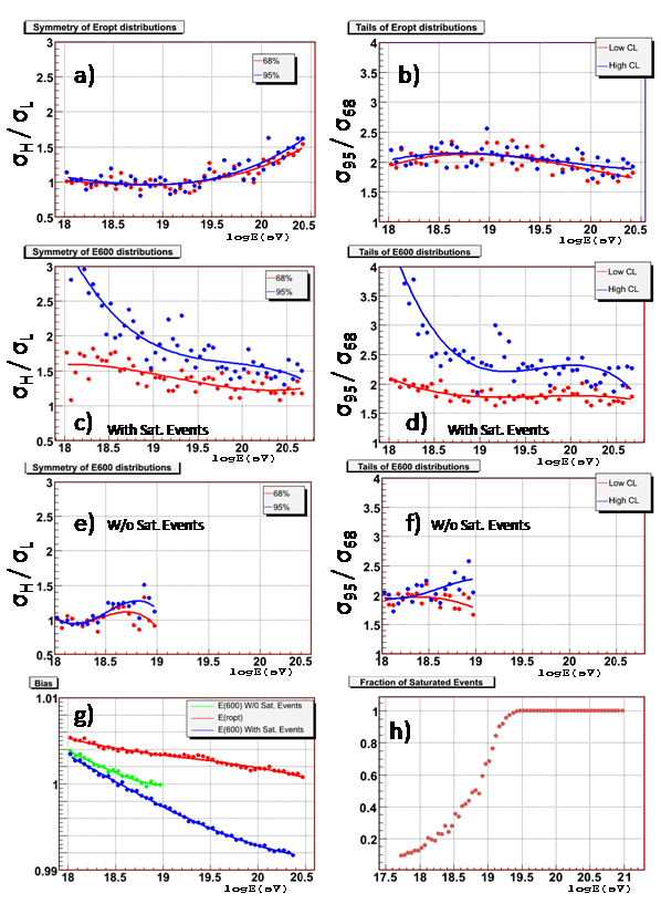
Figure 2: From a) to f): Fist row is for E($r_{opt}$), the second row is for E(600) with saturated events and the third row is for E(600) without saturated events; left column are the symmetry of the distributions comparing their high and low sides (Gaussian $\sigma_{H}/\sigma_{L}=1$) and right column are the tails of the distributions comparing their C.L. at 68% and 95% (Gaussian $\sigma_{95}/\sigma_{68}=2$). (g) reconstructed energy bias. (h) fraction of saturated events.

It is important to emphasize two things. First, in both cases, $S_{\theta}(600)$ and $S(r_{opt})$, the $\chi^{2}/ndof$ of the corresponding fits are very good (at the level of $10^{-2}$). Second, in the case of $S_{\theta}(600)$, the energy reconstruction is very bad for events with one or more saturated stations and energy below $10^{18.5}\;eV$ so they were rejected to improve reconstruction. This problem does not happen with $S(r_{opt})$, highlighting a major advantage of the latter method.

Figure 3: Spectrum input (black) with the same statistic as AGASA and the reconstructed one obtained using $S_{0}(600)$ ($S(r_{opt})$) as energy estimator in blue (red). In green is the spectrum obtained using $S_{0}(600)$ but rejecting saturated events. The vertical axis is multiplied by $E^{3}$. Error bars are the CL at 68 and 95% with 112 spectrums.

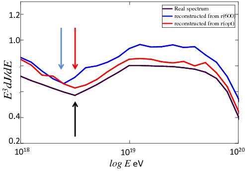
Figure 4: Input structured spectrum (black) and the reconstructed spectra using $S_{0}(600)$ (blue) and $S(r_{opt})$ (red) as energy estimator note the position of the ankle and the GZK transition.

Figure 4 shows the effects of both energy reconstructions when applied to a realistically structured spectrum (black curve), that has a an ankle, a GZK modulation, observed by an array with $\tanh$ acceptance that attains full efficiency $\lesssim 10^{18}$ eV. It can be seen that while the $S(r_{opt})$ method fairly reproduces the impinging spectrum, the $S_{\theta}(600)$ method changes the position of the ankle and smoothes the GZK transition.

Therefore, using an optimum distance, calculated for each individual shower to estimate primary energy is a simple procedure to improve the reliability of the calculated spectrum. Additionally, the $r_{opt}$ strategy minimizes the dead-time introduced by saturated stations or the possible biases originated by the implementation of algorithms designed to recover saturated signals.

4 Acknowledgements

G. Ros thanks the Comunidad de Madrid for a F.P.I. fellowship and the HELEN program. This work is partially supported by Spanish grants FPA2006-12184-C02, CAM/UAH2005/071, CCG06-UAH/ESP-0397, and Mexican PAPIIT/CIC, UNAM.

References

- [1] A. M. Hillas. Acta Phys. Acad. Sci. Hung., 29, Suppl. 3, 355 (1970).
- [2] Takeda et al. Ap. Phys. 19 (2003) 447.
- [3] G. A. Medina-Tanco et al. Proceedings of th 29th ICRC, Pune, 7, (2005) 43.
- [4] Pierre Auger Collaboration. NIM, 523, (2004) 50.
- [5] M. C. Medina et al. NIM A, 566, (2006) 302.
- [6] G. Ros et al. Resúmenes de la XXXI Reunión bienal de la RSEF, (2007).