Extreme statistics of complex random and quantum chaotic states

Abstract

An exact analytical description of extreme intensity statistics in complex random states is derived. These states have the statistical properties of the Gaussian and Circular Unitary Ensemble eigenstates of random matrix theory. Although the components are correlated by the normalization constraint, it is still possible to derive compact formulae for all values of the dimensionality $N$. The maximum intensity result slowly approaches the Gumbel distribution even though the variables are bounded, whereas the minimum intensity result rapidly approaches the Weibull distribution. Since random matrix theory is conjectured to be applicable to chaotic quantum systems, we calculate the extreme eigenfunction statistics for the standard map with parameters at which its classical map is fully chaotic. The statistical behaviors are consistent with the finite-$N$ formulae.

The study of the statistics of extreme values Gumbel (2004) has found many applications in diverse areas such as geophysics, metereology, economics, structural engineering, ocean waves, and dynamical systems. The subject is currently undergoing a resurgence of interest due to recent catastrophic events such as hurricanes, floods, and a particularly deadly tsunami as well as a number of research advances S. Albeverio (2006). The kinds of questions being asked are, for example, what are the distributions for extreme events, or what are the inter-event gap distributions. It has long been known that if the underlying events are independent and identically distributed, then for appropriately rescaled variables there are three possible limiting universal distributions for the extreme maximal events: the Fréchet, Gumbel and Weibull distributions Gumbel (2004). Respectively, they arise depending on whether the tail of the density is a power law, or faster than any power-law, and unbounded or bounded. If there are correlations, then it is known that these universal distributions are reached for a sufficiently fast decay of auto-correlations Leadbetter and Rootzen (1988).

In this letter, we apply these powerful methods to study the extreme properties of random vectors, or wave functions more generally, in the context of quantum mechanics. Our motivation is that the eigenstate intensities in fully chaotic systems with no particular symmetries are conjectured to behave exactly as these random vectors subject only to a normalization constraint as in random matrix theory. For chaotic systems, the applicability of random matrix theory Mehta (2004); Brody et al. (1981) has been well appreciated since the Bohigas-Giannoni-Schmit conjecture which states that the spectral fluctuations of quantized classically chaotic systems can be modelled by a suitable ensemble of random matrices Bohigas et al. (1984). In fact, a certain number of extreme spectral properties have already been derived Majumdar and Krapivsky (2003); Györgyi et al. (2003); Dean and Majumdar (2006); Sabhapandit and Majumdar (2007) beginning with the well-known result for the distribution of the largest eigenvalue Tracy and Widom (1994, 1996). The corresponding treatment of random vectors or quantum eigenvectors has not yet been addressed. However, see Aurich et al. (1999) for an initial foray into random waves.

In fact, eigenstate intensities in strongly chaotic systems are known to follow an exponential density, which is consistent with states uniformly distributed over a standard simplex Bengtsson and Zyczkowski (2006), as happens in the Unitary Ensembles (if an anti-unitary symmetry is respected, Porter-Thomas density, hypersphere, and Orthogonal Ensembles Porter (1965)). A similar class of problems shows up in fragmentation, i.e. randomly cutting an object of fixed length into $N$ pieces Derrida and Flyvbjerg (1987).

It is possible to give compact, exact formulae for all dimensionality $N$ in spite of the correlations introduced by the normalization constraint. It turns out that the small-$N$ distributions for the maxima differ considerably from their asymptotic limit (which turns out to be Gumbel, $\exp[-{\rm e}^{-x}]$) thus giving the possibility of extracting system size from the distributions. In an $N$-dimensional complex Hilbert space a general state is represented in a fixed orthonormal basis $|i\rangle$ as $|\psi\rangle=\sum_{i=1}^{N}z_{i}|i\rangle$. If the $z_{i}$ are complex components of a random state, they are not constrained by any requirement other than normalization, and their joint probability distribution is:

$$P(z_{1},z_{2},\ldots,z_{N})=\dfrac{(N-1)!}{\pi^{N}}\delta\left(\sum_{j=1}^{N}|z_{j}|^{2}\,-\,1\right).$$ (1)

The real and imaginary parts of the components are spread in an unbiased, microcanonical, manner over the $2N$-dimensional unit sphere. The intensities $|z_{i}|^{2}$ are distributed uniformly on an $N-1$ simplex. Thus a random state is correlated by this requirement. Given such an ensemble of random states we consider the probability distribution $\rho(t,N)$ of $t=\mbox{max}\{|z_{1}|^{2},|z_{2}|^{2},\cdots,|z_{N}|^{2}\}$. Let $F(t,N)$ be the probability that all $|z_{j}|^{2}\leq t$. This is called the distribution or cumulative density of such extreme events, i.e. $F^{\prime}(t,N)=\rho(t,N)$ where the prime denotes differentiation with $t$. Thus

$$F(t,N)=\dfrac{(N-1)!}{(2\pi)^{N}}\prod^{N}_{i=1}\left[\int_{0}^{2\pi}d\theta_{i}\int_{0}^{t}dr_{i}^{2}\right]\delta\left(\sum_{j=1}^{N}r_{j}^{2}\,-\,1\right)$$ (2)

where $r_{j}\equiv|z_{j}|$. Use a Fourier decomposition of the $\delta$-function and perform the $\{\theta_{i},r_{i}\}$ integrals to arrive at

$$F(t,N)=\dfrac{(N-1)!}{2\pi}\int_{-\infty}^{\infty}d\xi e^{-i\xi}\left(\dfrac{e^{i\xi t}-1}{i\xi}\right)^{N}.$$ (3)

Next expand the power in a binomial series to find

$$F(t,N)=\dfrac{(N-1)!}{2\pi i^{N}}\sum_{m=0}^{N}\binom{N}{m}(-1)^{N-m}I(1-mt),$$ (4)

where

$$I(\omega)=\int_{-\infty}^{\infty}e^{-i\omega\xi}\xi^{-N}d\xi=\dfrac{\pi(-i)^{N}}{(N-1)!}\omega^{N-1}\,\mbox{sign}(\omega).$$ (5)

The exact result for $F(t,N)$ is

$$F(t,N)=\dfrac{1}{2}\sum_{m=0}^{N}\binom{N}{m}(-1)^{m}(1-mt)^{N-1}\mbox{sign}(1-mt).$$ (6)

Expanding the power again and using the identity Gradshteyn and Ryzhik (2000):

$$\sum_{m=0}^{N}\binom{N}{m}(-1)^{m}m^{k}=0,\;\;k=0,\ldots N-1$$ (7)

gives “resummed” expressions for $F(t,N)$ valid in the intervals $I_{k}=[1/(k+1),1/k]$, where $k=1,2,\cdots,N-1$:

$$F(t\in I_{k},N)=\sum_{m=0}^{k}\binom{N}{m}(-1)^{m}(1-mt)^{N-1},$$ (8)

and $F(t\leq 1/N,N)=0$. Thus the cumulative density is a piecewise smooth function on the intervals $I_{k}$.

Given the simple form of the distribution above, it is useful to interpret them combinatorially and derive them from such an approach. First note that

$$P_{l}(z_{1},z_{2},\ldots,z_{l})=\dfrac{\Gamma(N)}{\pi^{l}\Gamma(N-l)}\left(1-\sum_{j=1}^{l}|z_{j}|^{2}\right)^{N-l-1}$$ (9)

where $P_{l}$ is the reduced probability density for $l$ complex components ($P_{N}$ is identical to the full distribution $P$ above). If $t\in I_{1}=[1/2,1]$ there can be at most only one such component. Therefore, the fraction of states with a component larger than $t$ is exactly the fraction of components larger than $t$. Since the desired quantity is the fraction of states such that all components are less than $t$, it is the simply the complement:

$$F(t,N)=1-N\int_{|z|^{2}\geq t}P_{1}(z)dz$$ (10)

The factor $N$ accounts for multiplicity of choice of this one component. This integral is elementary for the complex case and gives $F(t,N)=1-N(1-t)^{N-1}$, which agrees with the series in the RHS of Eq. (8) which terminates at $k=1$ for $t\in I_{1}$.

If $t\in I_{2}$, it is possible that there are at most two such components. The number of components $\geq t$ is no longer the number of sequences (states) with at least one component more than $t$ as it double counts states which have two components larger than $t$, a contribution which must get subtracted. This same logic extends, and in the next interval $I_{3}$, the number of pairs over counts the contributions of triples. Similarly, this reasoning carries forward to any distribution with a unit norm constraint and gives for the cumulative density

$$F(t\in I_{k},N)=$$

$$\sum_{m=0}^{k}\binom{N}{m}(-1)^{m}\int_{|x_{i}|^{2}>t}P_{m}(x_{1},\ldots,x_{m})\,dx_{1}\cdots dx_{m},$$

which is the generalization of Eq. (8) (the $m=0$ term in the above expression is unity). This generalization could be used as the starting point for an analysis of real random states as well as general density matrix eigenvalues whose sum is also constrained to be unity. It is interesting that piecewise continuous extreme distributions have been identified in dynamical systems Balakrishnan et al. (1995); Nicolis et al. (2006) and fragmentation problems Derrida and Flyvbjerg (1987), where a similar combinatorial approach was also applied.

From the distribution Eq. (6) above, it is possible to derive exact formulae for the moments. In particular, results for the first (mean) and the second moments of the maximum components are

$$\langle t\rangle = \dfrac{H(N,1)}{N}=\dfrac{\gamma+\ln N}{N}+{\mathcal{O}}\left(\dfrac{1}{N^{2}}\right)$$ (12)

$$\langle t^{2}\rangle = \dfrac{H^{2}(N,1)+H(N,2)}{N(N+1)}$$ (13)

where $H(N,k)$ is the Harmonic number of order $k$ defined by the finite sum $\sum_{m=1}^{N}m^{-k}$, and $\gamma=0.5772\cdots$ is the Euler-Mascheroni constant. The standard deviation can be calculated exactly and its large-$N$ form is:

$$\sigma(t)=\dfrac{\pi}{\sqrt{6}N}+{\mathcal{O}}\left(\dfrac{\ln(N)}{N}\right)^{2}.$$ (14)

It turns out that the asymptotic $N\rightarrow\infty$ limit here is also the result for uncorrelated exponentially distributed variables of mean $1/N$. This limit may be calculated by simply taking $P_{1}$ as the probability density of an independent process, which gives

$$F(t,N\rightarrow\infty)=\left(1-e^{-Nt}\right)^{N}\approx\exp\left(-e^{-N[t-\ln N/N]}\right).$$ (15)

Expressed in terms of the standard linearly scaled variable $x=(t-a_{N})/b_{N}$, this distribution is seen to coincide with the Gumbel distribution where the parameters are given by $a_{N}=\ln(N)/N$ and $b_{N}=1/N$. As should happen, the mean and the standard deviation calculated from the Gumbel distribution coincide with the leading order contributions derived in Eqs.(12,14).

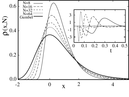
Figure 1: The convergence of the exact probability density to the asymptotic Gumbel distribution using the scaled variable $x=N(t-\ln(N)/N)$ with increasing $N$. The inset shows the difference between the exact and the Gumbel distribution for the same values of $N$, but in the unscaled variable.

That the maximal statistics is a Gumbel distribution is interesting because the intensities have a finite support, being constrained to lie on the standard $N-1$-simplex. The expectation for uncorrelated bounded variables would be the Weibull distribution; however the correlations introduced by the normalization constraint transforms this to the Gumbel distribution. In Fig. (1) we compare the exact probability density with that of the Gumbel density ($\exp[-x-e^{-x}]$) after appropriately rescaling. It is clear that the approach of the exact density to the Gumbel one is rather slow and at $N$ around $100$ there are still significant differences between the asymptotic and the exact. It is also instructive to note that without the rescaling the densities actually diverge as $N$ increases. This difference gives the possibility of extracting system size information from the extreme statistics.

The distribution of the minimum intensity $s=\mbox{min}\{|z_{1}|^{2},|z_{2}|^{2},\cdots,|z_{N}|^{2}\}$ on the other hand is a much simpler quantity and is not asymptotically a Gumbel distribution. The fraction of states such that the minimum is larger than some $s$ is the fraction of states such that all the components are larger than $s$. Thus if $F(s,N)$ is the cumulative distribution of the minimum, it is given by

$$F(s,N)=1-\dfrac{(N-1)!}{(2\pi)^{N}}\prod_{i=1}^{N}\left[\int_{0}^{2\pi}d\theta_{i}\int_{s}^{1}dr_{i}^{2}\right]\delta\left(\sum_{j=1}^{N}r_{j}^{2}\,-\,1\right),$$ (16)

which is very similar to the integral in Eq. (2). Its evaluation proceeds similarly to the maximum, and gives:

$$F(s,N)=\left\{\begin{array}[]{ll}1-(1-Ns)^{N-1}&0\leq s\leq 1/N\\ 1&1/N\leq s\leq 1\end{array}\right..$$ (17)

It is clear that the minimum cannot exceed $1/N$, just as the maximum cannot be less than this. The average minimum component is easily calculated and is exactly equal to $\langle s\rangle=1/N^{2}$. The distribution for the minimum does not have the piecewise continuous character we observed for the maximum. This has a geometrical interpretation in terms of the standard-simplex. In the case of the maximum the integral in Eq. (2) can be interpreted in terms of volumes of subsets contained in the region bounded by the standard $N-1$-simplex; these volumes enclosing more complex shapes for increasing $t$, as they pierce the simplex boundary. Whereas for the integral in Eq. (16) the volumes involved are those of the entire simplex and the volume of a subset that never pierces the $N-1$ simplex.

For large $N$ the distribution of the minimum approaches the exponential:

$$F(s,N\rightarrow\infty)=1-\exp(-N^{2}s).$$ (18)

This being a special case of the Weibull distribution, it is indeed what one would expect of uncorrelated variables with a compact support. That the minimum cannot be less than zero presents a strong constraint and for small components the normalization correlation is not so important. Thus, the distribution of the maximum and minimum of the complex random vector intensities follow different universal distributions asymptotically. It is noteworthy, however, that the limiting large deviations of the maximum component toward a small value which occur in the interval $I_{N-1}=1/N\leq t\leq 1/(N-1)$ is distributed as $F(t,N)=(Nt-1)^{N-1}$ which is an exact reflection about the value $1/N$ of the behavior of the minimum component.

In order to compare these extreme statistics to the statistical properties of the eigenfunctions of a Hamiltonian system, consider a quantum kicked rotor Izrailev (1990). This is a stroboscopic mapping of a kicked one-dimensional particle of unit mass moving on a circle of unit perimeter with the Hamiltonian $H(q,p)=p^{2}/2-(K/4\pi^{2})\cos(2\pi q)\sum_{n=-\infty}^{\infty}\delta(t-n)$. From $H(q,p)$, the classical mapping can be given Lichtenberg and Lieberman (1983) (modulo unity):

$$p_{i+1}=p_{i}-K/(2\pi)\sin(2\pi q_{i})\ ;\quad q_{i+1}=q_{i}+p_{i+1}$$ (19)

where the potential kick is applied before the free motion and the phase space is restricted to the unit torus ($q,p\in[0,1)$) for convenience. For $K\gg 5$ the map is highly chaotic, although the phase space almost always contains some tiny proportion of regular motion mixed in.

In the position basis, the evolution operator is

$$\begin{split}U_{nn^{\prime}}&=\frac{1}{N}\exp\left(\frac{iNK}{2\pi}\cos\left(\frac{2\pi(n^{\prime}+\alpha)}{N}\right)\right)\\ &\times\sum_{m=0}^{N-1}\exp\left(-\pi i\frac{(m+\beta)^{2}}{N}+\frac{2\pi i(m+\beta)(n-n^{\prime})}{N}\right).\end{split}$$ (20)

The two phases $0\leq\alpha,\beta\leq 1$ can be used for controlling parity and time-reversal symmetry breaking ($\alpha=1/2,\beta=0$ preserves both symmetries). Choosing $\beta$ well away from $0$ or $1/2$ breaks time-reversal invariance, which for $K\gg 5$ leads to quantum chaotic states that are complex and whose extremes should follow the distributions of the unitary ensembles.

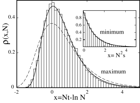
Figure 2: The probability densities (histograms) of the scaled maximum and minimum (inset) intensity of eigenfunctions in the position basis of the quantum kicked rotor for $N=32$ in the parameter range $13.8<K<14.8$. Shown as a continuous line is the exact density for random states while the dotted ones are the respective Gumbel and Weibull densities.

The dimensionality of the Hilbert space $N$ is the inverse (scaled) Planck constant.

An ensemble of roughly $30,000$ quantum chaotic eigenstates is created from the $N$ orthonormal states, as well as from those obtained by a variation of parameters $K$, $\alpha$, and $\beta$ such that while the quantum spectrum is significantly changed, the classical dynamics is not. Figure (2) shows the density of the maximal and minimal intensities in the position basis for a range of $K$ values where the classical map has no significant islands and is highly chaotic Tomsovic and Lakshminarayan (2007). The derivatives of the exact results in Eqs. (8,17) fit the quantum system histograms very well. The deviations are roughly of the scale of the expected sample size errors. Note that the dynamical system results require the exact density for the maximum as the asymptotic approach is too slow. This is in contrast to the exact finite-$N$ Dyson/Mehta fluctuation measures Mehta (2004), which approach their asymptotic limits so quickly that finite-$N$ results are rarely, if ever, used. The inset shows that the fit to the Weibull is excellent even for the small value of $N$ used. Given the excellent agreement of the dynamical systems results with the analytic forms, deviations may in turn be used to investigate the important issue of eigenstate localization.

In summary, recent years have seen a fast and fruitful development of the merging of extreme statistics tools and random matrix eigenvalues. This letter extends this general perspective to the properties of eigenvectors.

References

- Gumbel (2004) E. J. Gumbel, Statistics of Extremes (Dover Publications Inc., New York, 2004).
- S. Albeverio (2006) H. K. E. S. Albeverio, V. Jentsch, Extreme Events in Nature and Society (Springer, Berlin, 2006).
- Leadbetter and Rootzen (1988) M. R. Leadbetter and H. Rootzen, Ann. Probab. 16, 431 (1988).
- Mehta (2004) M. L. Mehta, Random Matrices (Third Edition) (Elsevier, Amsterdam, 2004).
- Brody et al. (1981) T. A. Brody, J. Flores, J. B. French, P. A. Mello, A. Pandey, and S. S. M. Wong, Rev. Mod. Phys. 53, 385 (1981).
- Bohigas et al. (1984) O. Bohigas, M. J. Giannoni, and C. Schmit, Phys. Rev. Lett. 52, 1 (1984).
- Majumdar and Krapivsky (2003) S. N. Majumdar and P. L. Krapivsky, Physica (Amsterdam) 318A, 161 (2003).
- Györgyi et al. (2003) G. Györgyi, P. C. W. Holdsworth, B. Portelli, and Z. Rácz, Phys. Rev. E 68, 056116 (2003).
- Dean and Majumdar (2006) D. S. Dean and S. N. Majumdar, Phys. Rev. Lett. 97, 160201 (2006).
- Sabhapandit and Majumdar (2007) S. Sabhapandit and S. N. Majumdar, Phys. Rev. Lett. 98, 140201 (2007).
- Tracy and Widom (1994) C. A. Tracy and H. Widom, Commun. Math. Phys. 159, 151 (1994).
- Tracy and Widom (1996) C. A. Tracy and H. Widom, Commun. Math. Phys. 177, 727 (1996).
- Aurich et al. (1999) R. Aurich, A. Bäcker, R. Schubert, and M. Taglieber, Physica 129D, 1 (1999).
- Bengtsson and Zyczkowski (2006) I. Bengtsson and K. Zyczkowski, Geometry of Quantum States (Cambridge Univ. Press, New York, 2006), links at http://en.wikipedia.org/wiki/Simplex.
- Porter (1965) C. E. Porter, Statistical Theories of Spectra: Fluctuations (Academic Press, New York, 1965).
- Derrida and Flyvbjerg (1987) B. Derrida and H. Flyvbjerg, J. Phys. A: Math. Gen. 20, 5273 (1987).
- Gradshteyn and Ryzhik (2000) I. S. Gradshteyn and I. M. Ryzhik, Table of Integrals, Series, and Products (Academic Press, San Diego, 2000).
- Balakrishnan et al. (1995) V. Balakrishnan, C. Nicolis, and G. Nicolis, J. Stat. Phys. 80, 307 (1995).
- Nicolis et al. (2006) C. Nicolis, V. Balakrishnan, and G. Nicolis, Phys. Rev. Lett. 97, 210602 (2006).
- Izrailev (1990) F. M. Izrailev, Phys. Rep. 196, 299 (1990).
- Lichtenberg and Lieberman (1983) A. J. Lichtenberg and M. A. Lieberman, Regular and Stochastic Motion (Springer, Berlin, 1983).
- Tomsovic and Lakshminarayan (2007) S. Tomsovic and A. Lakshminarayan, Archive: p. 0706.1494 (2007).