HTL approach to the viscosity of quark plasma

Abstract

The quark viscosity in the quark gluon plasma is evaluated in HTL approximation. The different contributions to the viscosity arising from the various components of the quark spectral function are discussed. The calculation is extended to finite values of the chemical potential.

In this letter we present a microscopic calculation of the shear viscosity $\eta$ and of its ratio to the entropy density $s$ for a system of quarks. This subject has been widely discussed in recent times, on the basis of the intriguing results from the experiments carried out at the Relativistic Heavy Ion Collider (RHIC). In particular the measurement of the $v_{2}$ coefficient [1] in the multipole analysis of the angular distribution of the produced hadrons seems to imply a very small viscosity, like the one of an almost perfect fluid [2, 3, 4], in contrast with the current description of the QGP as a gas of weakly interacting quasi-particles [5]. The substantial collective flow observed in these collisions also seems to imply quite small values for the viscosity [6, 7, 8, 9, 10].

The temperature behavior of the ratio $\eta/s$ should determine the value $T_{c}$ at which a phase transition occurs in the system [4, 10]. Much emphasis has received the result of certain special supersymmetric Yang-Mills theories in 4 dimensions, which predicts a lower limit for the viscosity/entropy density ratio, namely $\eta/s\geq 1/4\pi$ (in units $\hbar=k_{B}=c=1$) [11, 12]; the latter value is approached by several recent calculations [13, 14, 15, 16]. Transport coefficients from the linearized Boltzmann equation for a non abelian gauge theory have been obtained using perturbative QCD in Refs. [17, 18].

Here we shall describe the quarks in the QGP within the Hard Thermal Loop (HTL) approximation, which has already been proven quite successful for the thermodynamics of high temperature QGP [19, 20, 21]. Quark-antiquark correlators have also been widely considered in this approach (see, e.g., Refs. [22, 23, 24] and references therein).

We evaluate the shear viscosity $\eta$ of the system limiting ourselves to the quark degrees of freedom and starting from the Kubo formulas for the hydrodynamic transport coefficients; it is expressed in terms of the correlator of the energy-momentum tensor as follows:

$$\eta=\lim_{\omega\to 0^{+}}\eta(\omega)=-\left.\frac{{\mathrm{d}}}{{\mathrm{d}}\omega}{\mathrm{Im}}\,\Pi^{R}(\omega)\right|_{\omega=0^{+}}\,,$$ (1)

where we consider the following retarded correlator (at zero momentum) [16]

$$\Pi^{R}(i\omega_{l})=N_{c}N_{f}\,\,\frac{1}{\beta}\sum_{n=-\infty}^{+\infty}\,\,\int\!\frac{d^{3}k}{(2\pi)^{3}}\,\,k_{x}^{2}\,\,\textrm{Tr}[\gamma_{2}\,S(i\omega_{n},k)\gamma_{2}\,S(i\omega_{n}\!-i\omega_{l},k)]\;.$$ (2)

In the above $\omega_{l}=2\pi l/\beta$, $\omega_{n}=(2n+1)\pi/\beta$, ($\beta=1/T$) are Matsubara frequencies and the spectral representation of the massless quark propagator is employed

$$S(i\omega_{n},k)=-\int\limits_{-\infty}^{+\infty}\!\frac{d\omega}{2\pi}\,\,\frac{{\rho(\omega,k)}}{i\omega_{n}-\omega}\;,$$ (3)

the spectral function being conveniently split into the chirality projections:

$$\rho(\omega,k)=\frac{\gamma^{0}-\mathbf{{\bm{\upgamma}}\cdot\hat{k}}}{2}\rho_{+}(\omega,k)\,+\,\frac{\gamma^{0}+\mathbf{{\bm{\upgamma}}\cdot\hat{k}}}{2}\rho_{-}(\omega,k)\;.$$ (4)

The explicit expression of the HTL quark spectral function introduced in Eq.(4) reads [25]:

$$\rho_{\pm}(\omega,k)=2\pi Z_{\pm}(k)[\delta(\omega-\omega_{\pm})+\delta(\omega+\omega_{\mp})]+2\pi\beta_{\pm}(\omega,k)\theta(k^{2}-\omega^{2})\;,$$ (5)

where $m_{q}=g(T)T/\sqrt{6}$ is the quark thermal mass,

$$Z_{\pm}(k)=\frac{\omega_{\pm}^{2}(k)-k^{2}}{2m_{q}^{2}}$$ (6)

are the residues of the quasi-particle poles [see Eq. (9)] and

$$\beta_{\pm}(\omega,k)=-\frac{m_{q}^{2}}{2}\times$$ (7)

$$\frac{\pm\omega-k}{\displaystyle{\left\{k(-\omega\pm k)+m_{q}^{2}\left[\pm 1-\left(\frac{\pm\omega-k}{2k}\right)\ln\frac{k+\omega}{k-\omega}\right]\right\}^{2}+\left\{\frac{\pi}{2}m_{q}^{2}\,\left(\frac{\pm\omega-k}{k}\right)\right\}^{2}}}\;.$$

The spectral functions $\rho_{\pm}(\omega,k)$ consist of two pieces, a pole term and a cut:

$$\rho_{\pm}(\omega,k)=\rho_{\pm}^{QP}(\omega,k)+\rho_{\pm}^{LD}(\omega,k)~{}.$$ (8)

At a given value of the spatial momentum $k$, in the time-like domain ($\omega^{2}>k^{2}$) discrete poles are associated to quasiparticle (QP) excitations with dispersion relation $\omega=\omega_{\pm}(k)$, while in the space-like domain ($\omega^{2}<k^{2}$) a cut accounts for the Landau damping (LD) of a quark propagating in the thermal bath. The two poles correspond to quasi-particles with opposite chirality/helicity sign, their dispersion relation being given by the solutions of the implicit equation:

$$\omega_{\pm}=\pm p+\frac{m_{q}^{2}}{2p}\left[\left(1\mp\frac{\omega_{\pm}}{p}\right)\ln\left|\frac{\omega_{\pm}+p}{\omega_{\pm}-p}\right|\pm 2\right].$$ (9)

Vertex corrections to the correlator (2) deserve further investigation and will not be included here.

We can now insert the spectral representation, Eq.(3), of the propagators into Eq.(2) and sum over the Matsubara frequencies with a standard contour integration; then, by performing the usual analytic continuation $i\omega_{l}\rightarrow\omega+i\eta^{+}$ (retarded boundary conditions), taking the imaginary part of the result and putting into Eq.(1) we obtain [15, 16]:

$$\eta=\frac{N_{c}N_{f}}{2T}\int\frac{d^{3}k}{(2\pi)^{3}}\,k^{2}_{x}\int_{-\infty}^{+\infty}\frac{d\omega}{2\pi}[1-f(\omega)]f(\omega)\,{\mathrm{Tr}}\left[\gamma^{2}\rho(\omega,{\bf k})\gamma^{2}\rho(\omega,{\bf k})\right]\,,$$ (10)

where $f(\omega)=1/(\exp^{\beta(\omega-\mu)}+1)$ is the thermal distribution for fermions with chemical potential $\mu$.

The trace over spin can be explicitly carried out after inserting Eq. (4) into Eq. (10) and, since

$$\textrm{Tr}\left[\gamma_{2}\frac{\gamma^{0}\mp\mathbf{{\bm{\upgamma}}\cdot\hat{k}}}{2}\gamma_{2}\frac{\gamma^{0}\mp\mathbf{{\bm{\upgamma}}\cdot\hat{k}}}{2}\right]=2\hat{k}_{y}^{2},\quad\textrm{Tr}\left[\gamma_{2}\frac{\gamma^{0}\mp\mathbf{{\bm{\upgamma}}\cdot\hat{k}}}{2}\gamma_{2}\frac{\gamma^{0}\pm\mathbf{{\bm{\upgamma}}\cdot\hat{k}}}{2}\right]=2-2\hat{k}_{y}^{2}\;,$$ (11)

one finally gets:

$$\eta =\frac{N_{c}N_{f}}{60\pi^{3}T}\int\limits_{0}^{+\infty}dk\,k^{4}\times$$

$$\int\limits_{-\infty}^{+\infty}d\omega\,[1-f(\omega)]f(\omega)\left\{\rho_{+}^{2}(\omega,{\bf k})+\rho_{-}^{2}(\omega,{\bf k})+8\rho_{+}(\omega,{\bf k})\rho_{-}(\omega,{\bf k})\right\}~{}.$$

By inserting the explicit expressions for $\rho_{\pm}(\omega,k)$ into Eq. (HTL approach to the viscosity of quark plasma) this quantity turns out to be split, in the HTL approximation, into three different contributions [pole-pole term, labelled QP, pole-cut term (QPLD) which mixes quasi-particle and Landau damping parts and cut-cut (LD) which comes from Landau damping only]:

$$\eta=\eta^{QP}+\eta^{QPLD}+\eta^{LD}~{}.$$ (13)

The quasi-particle (pole-pole) contribution reads:

$$\eta^{QP} = \frac{N_{c}N_{f}}{60\pi^{3}T}\int\limits_{0}^{+\infty}dk\,k^{4}\int\limits_{-\infty}^{+\infty}d\omega\,[1-f(\omega)]f(\omega)\left\{\rho_{+}^{QP}(\omega,{\bf k})-\rho_{-}^{QP}(\omega,{\bf k})\right\}^{2}$$ (14)

$$+ \frac{N_{c}N_{f}}{60\pi^{3}T}\int\limits_{0}^{T}dk\,k^{4}\int\limits_{-\infty}^{+\infty}d\omega\,[1-f(\omega)]f(\omega)\left\{10\rho_{+}^{QP}(\omega,{\bf k})\rho_{-}^{QP}(\omega,{\bf k})\right\}~{}.$$

The Landau damping (cut-cut) contribution reads:

$$\eta^{LD} = \frac{N_{c}N_{f}}{60\pi^{3}T}\int\limits_{0}^{+\infty}dk\,k^{4}\int\limits_{-k}^{+k}d\omega\,[1-f(\omega)]f(\omega)\times$$

$$\times \left\{[\rho_{+}^{LD}(\omega,{\bf k})-\rho_{-}^{LD}(\omega,{\bf k})]^{2}+10\rho_{+}^{LD}(\omega,{\bf k})\rho_{-}^{LD}(\omega,{\bf k})\right\}$$

and finally the pole-cut contribution reads:

$$\eta^{QPLD} = \frac{N_{c}N_{f}}{60\pi^{3}T}\int\limits_{0}^{+\infty}dk\,k^{4}\int\limits_{-k}^{+k}d\omega\,[1-f(\omega)]f(\omega)\times$$

$$\times \left\{2\rho_{+}^{QP}(\omega,{\bf k})\rho_{+}^{LD}(\omega,{\bf k})+2\rho_{-}^{QP}(\omega,{\bf k})\rho_{-}^{LD}(\omega,{\bf k})\right.$$

$$+ \left.8\rho_{+}^{QP}(\omega,{\bf k})\rho_{-}^{LD}(\omega,{\bf k})+8\rho_{-}^{QP}(\omega,{\bf k})\rho_{+}^{LD}(\omega,{\bf k})\right\}~{}.$$

Among the three contributions, the QP one, as it stands, turns out to be divergent, as it corresponds to a free gas of particles. In order to cure this unphysical outcome, we shall assign, following Ref. [26], a finite width to the poles keeping unchanged the residues: the width of the poles $\pm\omega_{+}(k)$ is $\gamma_{+}$ and the width of $\pm\omega_{-}(k)$ is $\gamma_{-}$. The spectral function for these dressed quasiparticles then reads:

$$\rho_{\pm}^{\textrm{QP}}(\omega,{\bf k})=Z_{\pm}(k)\frac{2\gamma_{\pm}}{[\omega-\omega_{\pm}(k)]^{2}+\gamma_{\pm}^{2}}+Z_{\mp}(k)\frac{2\gamma_{\mp}}{[\omega+\omega_{\mp}(k)]^{2}+\gamma_{\mp}^{2}}$$ (17)

and is normalized according to

$$\int\limits_{-\infty}^{+\infty}\frac{d\omega}{2\pi}\rho_{\pm}^{\textrm{QP}}(\omega,{\bf k})=Z_{+}(k)+Z_{-}(k)~{}.$$ (18)

The width is fixed as in Ref. [26]:

$$\gamma_{\pm}=a\frac{C_{f}g^{2}T}{16\pi},$$ (19)

where $a=3.0$ is chosen as an intermediate value between the one loop calculation and the improved one of Ref. [26] for $N_{f}=2$. $C_{f}=4/3$ is the Casimir constant for the fundamental representation of SU($N_{f}$). A word of caution is in order with the use of a constant quasi-particle width: indeed, as observed in Ref. [16], the second term of $\eta^{QP}$ [second line in Eq. (14)] would contain an ultraviolet divergence. A natural cutoff is provided by the scale of momenta within the HTL approach, since the particles dressed by HTL self-energy are expected to be “soft” constituents, where the soft momenta are defined as the ones smaller than $T$ (or $gT$). Hence the upper limit of the integration over $k$ in the second line of Eq. (14) has been set to $T$.

In addition to the shear viscosity, we have then evaluated the entropy density according to the formulas of Ref. [20, 21].

The ratio $\eta/s$ is illustrated in Fig. 1 (solid line) for $\mu=0$ as a function of $T/T_{c}$, with $T_{c}=202$ MeV, which was suggested as the transition temperature for $N_{f}=2$ in Ref. [27]. Moreover we use the temperature dependent running gauge coupling given by the two-loop perturbative beta-function [5, 28, 29, 23]. In the same figure we display the separate contributions from $\eta^{QP}$, $\eta^{QPLD}$ and $\eta^{LD}$. Clearly the dominant contribution is $\eta^{QP}$: we notice that the cutoff dependence in the second term of the QP contribution is quite mild, since the first term is by far dominant; indeed by artificially increasing the cutoff up to $10T$ the ratio $\eta/s$ increases by about $2\%$. We wish to stress that the contribution of the continuum to the viscosity was never evaluated in previous works: we find that it is quite small and that its temperature dependence is opposite to the QP one, showing a fast decrease, which is also reflected in the QP-LD interference term.

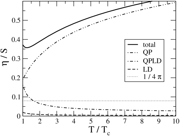
Figure 1: The ratio $\eta/s$ for $\mu=0$ as a function of $T/T_{c}$: the QP (dash-double-dotted line), LD (dashed) and the interference between QP and LD (dot-dashed) are shown, together with the total result (solid). The limit $1/4\pi$ is indicated by the dotted line.

We have then extended our calculation of $s$, $\eta$ and $\eta/s$ to the case of finite chemical potential, taking also into account the corresponding correction to the quark mass [30],   $m_{q}^{2}={g^{2}(T)}\left(T^{2}+{\mu^{2}}/{\pi^{2}}\right)/{6}$. Finite baryonic densities in high energy heavy ion collisions will be of interest for the forthcoming GSI experiments. The ratio of the entropy density to the corresponding Stefan-Boltzmann limit ($s_{\mathrm{free}}$) is shown in Fig. 2 for three different values of $\mu$: the curves corresponding to $\mu\neq 0$ have been extended to lower temperatures, since $T_{c}$ should gradually decrease with increasing chemical potential. The effect of the chemical potential appears to be sizable only for the largest value considered here.

In Fig. 3 we display the $\eta/s$ ratio for different values of $\mu$: one can see that the effect of a finite chemical potential increases the ratio, which implies a larger correction to the viscosity than to the entropy density (the modification of the latter, according to the results shown in Fig. 2, should lower $\eta/s$). Obviously the largest effects are seen at lower temperatures.

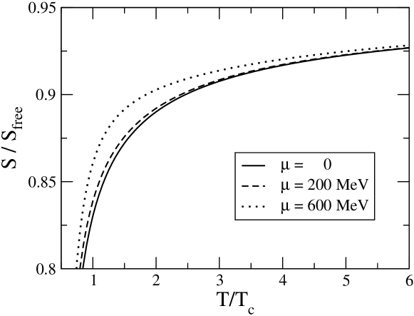
Figure 2: Entropy density of quarks in HTL approximation (divided by $s_{\mathrm{free}}$) as a function of $T/T_{c}$ for $\mu=0$ (solid line), $\mu=200$ MeV (dashed) and $\mu=400$ MeV (dotted).

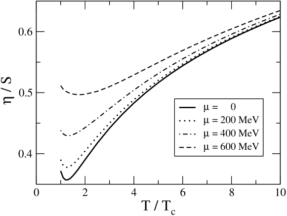
Figure 3: The ratio $\eta/s$ as a function of $T/T_{c}$ for different values of the chemical potential: $\mu=0$ (solid line), $\mu=200$ MeV (dotted), $\mu=400$ MeV (dot-dashed) and $\mu=600$ MeV (dashed).

In summary we have microscopically calculated the viscosity and the entropy density for a system of quarks described in the framework of the HTL approximation. The quasi-particle term in the spectral density has been modified by accounting, within the same approach, for a finite width, which removes the divergence in the shear viscosity derived from the Kubo formula. The results for the $\eta/s$ ratio are comparable to the ones obtained within phenomenological models [16] and turn out to be about a factor 3 larger than recent lattice calculations [14] in the pure gauge sector. We found that the continuum part of the quark spectral density gives a negligible contribution to the viscosity and the corresponding $\eta/s$ ratio slowly decreases with temperature, at variance with the dominant, quasi-particle one.

We have also considered the effect of a finite chemical potential and we found that it causes a sizable increase, both in the entropy density and in the viscosity: indeed $\mu$ induces the largest corrections to the latter, so that also the ratio $\eta/s$ tends to increase with the chemical potential.

Acknowledgments One of the authors (P.C.) thanks the Department of Theoretical Physics of the Torino University and INFN, Sezione di Torino, for the warm hospitality.

References

- [1] S. S. Adler, et al. (PHENIX Collaboration), Phys. Rev. Lett. 91 (2003) 182301; J. Adams, et al. (STAR Collaboration), Phys. Rev. C 72 (2005) 014904; B. B. Back, et al. (PHOBOS Collaboration), Phys. Rev. C 72 (2005) 051901(R); A. Adare et al. (PHENIX Collaboration), Phys. Rev. Lett. 98 (2007) 172301.
- [2] P. Huovinen, P. F. Kolb, U. W. Heinz, P. V. Ruuskanen and S. A. Voloshin, Phys. Lett. B 503 (2001) 58.
- [3] H. J. N. Drescher, A. Dumitru, C. Gombeaud and J. Y. Ollitrault, arXiv:nucl-th/0704.3553.
- [4] L. P. Csernai, J. I. Kapusta and L. D. McLerran, Phys. Rev. Lett. 97 (2006) 152303.
- [5] F. Karsch, E. Laermann and A. Peikert, Phys. Lett. B478 (2000) 447.
- [6] D. Teaney, J. Lauret and E. V. Shuryak, Nucl. Phys. A 698 (2002) 479.
- [7] D. Teaney, Phys. Rev. C 68 (2003) 034913.
- [8] A. Peshier and W. Cassing, Phys. Rev. Lett. 94 (2005) 172301.
- [9] J. I. Kapusta, arXiv:0705.1277 [nucl-th].
- [10] R. A. Lacey et al., Phys. Rev. Lett. 98 (2007) 092301.
- [11] G. Policastro, D. T. Son and A. O. Starinets, Phys. Rev. Lett. 87 (2001) 081601.
- [12] P. Kovtun, D. T. Son and A. O. Starinets, Phys. Rev. Lett. 94 (2005) 111601.
- [13] A. Nakamura and S. Sakai, Phys. Rev. Lett. 94 (2005) 072305.
- [14] H. B. Meyer, arXiv:0704.1801 [hep-lat].
- [15] M. Iwasaki, H. Ohnishi and T. Fukutome, arXiv:hep-ph/0606192 and arXiv:hep-ph/0703271.
- [16] W. M. Alberico, S. Chiacchiera, H. Hansen, A. Molinari and M. Nardi, arXiv:0707.4442 [hep-ph].
- [17] P. Arnold, G. D. Moore and L. G. Yaffe, JHEP 0011 (2000) 001.
- [18] P. Arnold, G. D. Moore and L. G. Yaffe, JHEP 0305 (2003) 051.
- [19] J. P. Blaizot, E. Iancu and A. Rebhan, Phys. Rev. Lett. 83 (1999) 2906.
- [20] J.P. Blaizot, E. Iancu and A. Rebhan, Phys. Lett. B 470 (1999) 181.
- [21] J.P. Blaizot and E. Iancu, Phys. Rev. D 63 (2001) 065003.
- [22] W. M. Alberico, A. Beraudo and A. Molinari, Nucl. Phys. A 750 (2005) 359.
- [23] W. M. Alberico, A. Beraudo, P. Czerski and A. Molinari, Nucl. Phys. A 775 (2006) 188.
- [24] W. M. Alberico, A. Beraudo, A. Czerska, P. Czerski and A. Molinari, Nucl. Phys. A 792 (2007) 152.
- [25] M. Le Bellac, Thermal Field Theory, Cambridge University Press, 1996.
- [26] E. Braaten, R. D. Pisarski, Phys.Rev. D46 (1992) 1829.
- [27] O. Kaczmarek, F. Zantow, Phys. Rev. D 71 (2005) 114510.
- [28] M. Gockeler et al., Phys.Rev. D73 (2006) 014513.
- [29] O. Kaczmarek and F. Zantow, hep-lat/0512031.
- [30] J.-P. Blaizot, E. Iancu, A. Rebhan, AIP Conf. Proc. - December 2, 2004 - Volume 739, pp. 63-96, Hwa, R.C. et al. (ed.) [e-Print: hep-ph/0303185].