Abstract

In this article, we take the point of view that the $D_{s}(2700)$ be a tetraquark state, which consists of a scalar diquark and a vector antidiquark, and calculate its mass with the QCD sum rules. The numerical result indicates that the mass of the vector charmed tetraquark state is about $M_{V}=(3.75\pm 0.18)\rm{GeV}$ or $M_{V}=(3.71\pm 0.15)\rm{GeV}$ from different sum rules, which is about $1\rm{GeV}$ larger than the experimental data. Such tetraquark component should be very small in the $D_{s}(2700)$.

PACS number: 12.38.Aw, 14.40.Lb

Key words: $D_{s}(2700)$, QCD sum rules

1 Introduction

Recently Belle Collaboration observed a new resonance $D_{s}(2700)$ in the decay $B^{+}\to\bar{D}^{0}D_{s}(2700)\to\bar{D}^{0}D^{0}K^{+}$. The resonance has the mass $M_{V}=2708\pm 9^{+11}_{-10}\rm{MeV}$, width $\Gamma_{V}=108\pm 23^{+36}_{-31}~{}\rm{MeV}$, and spin-parity $1^{-}$[1]. They interpret the $D_{s}(2700)$ as a $c\bar{s}$ meson, the potential model calculations predict a radially excited $2^{3}S_{1}$ ($c\bar{s}$) state with a mass about $(2710-2720)\rm{MeV}$ [2]. The resonance $D_{s}(2700)$ is consistent with the particle they presented previously in the 33rd international conference on high energy physics (ICHEP 06), $M_{V}=2715\pm 11^{+11}_{-14}\rm{MeV}$, $\Gamma_{V}=115\pm 20^{+36}_{-32}\rm{MeV}$ and spin-parity $1^{-}$ [3]. In the same analysis of the $DK$ mass distribution, Babar Collaboration observed a broad structure with $M_{V}=2688\pm 4\pm 3\rm{MeV}$ and $\Gamma_{V}=112\pm 7\pm 36\rm{MeV}$, which maybe the same resonance observed by Belle Collaboration [4] .

In this article, we take the point of view that the vector charmed meson $D_{s}(2700)$ be a tetraquark state, which consists of a scalar diquark and a vector antidiquark, and devote to calculate its mass with the QCD sum rules [5, 6]. The $D_{s}(2700)$ lies above the $DK$ threshold, the decay $D_{s}(2700)\to D^{0}K^{+}$ can take place with the fall-apart mechanism and it is OZI super-allowed, which can take into account the large width naturally. Furthermore, whether or not there exists such a tetraquark configuration which can result in the state $D_{s}(2700)$ is of great importance itself, because it provides a new opportunity for a deeper understanding of low energy QCD. We explore this possibility, later experimental data can confirm or reject this assumption.

The article is arranged as follows: we derive the QCD sum rules for the mass of the $D_{s}(2700)$ in section 2; in section 3, numerical result and discussion; section 4 is reserved for conclusion.

2 QCD sum rules for the mass of the $D_{s}(2700)$

In the following, we write down the two-point correlation function $\Pi_{\mu\nu}(p)$ in the QCD sum rules,

$$\Pi_{\mu\nu}(p) = i\int d^{4}xe^{ip\cdot x}\langle 0|T\left\{J_{\mu}(x)J^{+}_{\nu}(0)\right\}|0\rangle\,,$$ (1)

$$J_{\mu}(x) = \frac{\epsilon_{kij}\epsilon_{kmn}}{\sqrt{2}}\left\{u^{T}_{i}(x)C\gamma_{5}c_{j}(x)\bar{u}_{m}(x)\gamma_{5}\gamma_{\mu}C\bar{s}^{T}_{n}(x)+(u\rightarrow d)\right\}\,.$$ (2)

We choose the vector current $J_{\mu}(x)$ which constructed from a scalar diquark and a vector antidiquark to interpolate the vector meson $D_{s}(2700)$.

Here we take a digression to discuss how to choose the interpolating currents for the tetraquark states. We can take either $qq-\bar{q}\bar{q}$ type or $\bar{q}q-\bar{q}q$ type currents to interpolate the tetraquark states, they are related to each other via Fierz transformation both in the Dirac spinor and color space [7, 8]. In this article, we take the $qq-\bar{q}\bar{q}$ type interpolating current.

The diquarks have five Dirac tensor structures, scalar $C\gamma_{5}$, pseudoscalar $C$, vector $C\gamma_{\mu}\gamma_{5}$, axial vector $C\gamma_{\mu}$ and tensor $C\sigma_{\mu\nu}$. From those diquarks, we can construct six independent currents to interpolating the charmed tetraquark states with $1^{-}$,

$$J^{1}_{\mu}(x) = \frac{\epsilon_{kij}\epsilon_{kmn}}{\sqrt{2}}\left\{u^{T}_{i}(x)C\gamma_{5}c_{j}(x)\bar{u}_{m}(x)\gamma_{5}\gamma_{\mu}C\bar{s}^{T}_{n}(x)+(u\rightarrow d)\right\}\,,$$

$$J^{2}_{\mu}(x) = \frac{\epsilon_{kij}\epsilon_{kmn}}{\sqrt{2}}\left\{u^{T}_{i}(x)C\gamma_{\mu}\gamma_{5}c_{j}(x)\bar{u}_{m}(x)\gamma_{5}C\bar{s}^{T}_{n}(x)+(u\rightarrow d)\right\}\,,$$

$$J^{3}_{\mu}(x) = \frac{\epsilon_{kij}\epsilon_{kmn}}{\sqrt{2}}\left\{u^{T}_{i}(x)Cc_{j}(x)\bar{u}_{m}(x)\gamma_{\mu}C\bar{s}^{T}_{n}(x)+(u\rightarrow d)\right\}\,,$$

$$J^{4}_{\mu}(x) = \frac{\epsilon_{kij}\epsilon_{kmn}}{\sqrt{2}}\left\{u^{T}_{i}(x)C\gamma_{\mu}c_{j}(x)\bar{u}_{m}(x)C\bar{s}^{T}_{n}(x)+(u\rightarrow d)\right\}\,,$$

$$J^{5}_{\mu}(x) = \frac{\epsilon_{kij}\epsilon_{kmn}}{\sqrt{2}}\left\{u^{T}_{i}(x)C\sigma_{\mu\nu}c_{j}(x)\bar{u}_{m}(x)\gamma_{5}\gamma_{\nu}C\bar{s}^{T}_{n}(x)+(u\rightarrow d)\right\}\,,$$

$$J^{6}_{\mu}(x) = \frac{\epsilon_{kij}\epsilon_{kmn}}{\sqrt{2}}\left\{u^{T}_{i}(x)C\gamma_{\nu}\gamma_{5}c_{j}(x)\bar{u}_{m}(x)\sigma_{\mu\nu}C\bar{s}^{T}_{n}(x)+(u\rightarrow d)\right\}\,,$$ (3)

and the general current $\widetilde{J}_{\mu}(x)$ can be written as their linear superposition,

$$\widetilde{J}_{\mu}(x) = \sum_{i=1}^{6}C_{i}J^{i}_{\mu}(x)\,,$$ (4)

where the $C_{i}$ are some coefficients.

The six interpolating currents can be sorted into three types, the currents $J^{1}_{\mu}(x)$ and $J^{2}_{\mu}(x)$ are $C\gamma_{5}-C\gamma_{\mu}\gamma_{5}$ type, the currents $J^{3}_{\mu}(x)$ and $J^{4}_{\mu}(x)$ are $C-C\gamma_{\mu}$ type, the currents $J^{5}_{\mu}(x)$ and $J^{6}_{\mu}(x)$ are $C\sigma_{\mu\nu}-C\gamma_{\nu}\gamma_{5}$ type. We expect the three type interpolating currents result in three type of masses for the tetraquark states.

The study with the random instanton liquid model indicates that the diquarks have masses about $m_{S}=420\pm 30\rm{MeV}$, $m_{A}=m_{V}=940\pm 20\rm{MeV}$, $m_{T}=570\pm 20\rm{MeV}$ [9], we expect the currents $J^{5}_{\mu}(x)$ and $J^{6}_{\mu}(x)$ interpolate the tetraquark states with masses larger than the ones for the currents $J^{1}_{\mu}(x)$ and $J^{2}_{\mu}(x)$. Instanton induced force results in strong attraction in the scalar diquark channels and strong repulsion in the pseudoscalar diquark channels, if the instantons manifest themselves, the pseudoscalar diquarks will have much larger masses than the corresponding scalar diquarks [10], the coupled Schwinger-Dyson equation and Bethe-Salpeter equation also indicate this fact [11]. Furthermore, the one-gluon exchange force leads to significant attraction between the quarks in the $0^{+}$ channels [10]. Although the interpolating currents are not unique, the currents $J^{1}_{\mu}(x)$ and $J^{2}_{\mu}(x)$ are much better and interpolate tetraquark states with smaller mass, we can choose either one of them.

In the conventional QCD sum rules [5], there are two criteria (pole dominance and convergence of the operator product expansion) for choosing the Borel parameter $M^{2}$ and threshold parameter $s_{0}$. For the tetraquark states, if the perturbative terms have the main contribution, we can approximate the spectral density with the perturbative term,

$$B_{M}\Pi\sim A\int_{0}^{\infty}s^{4}e^{-\frac{s}{M^{2}}}ds=AM^{10}\int_{0}^{\infty}t^{4}e^{-t}dt\,,$$ (5)

where the $A$ are some numerical coefficients, then we take the pole dominance condition,

$$\frac{\int_{0}^{t_{0}}t^{4}e^{-t}dt}{\int_{0}^{\infty}t^{4}e^{-t}dt}\geq 50\%\,,$$ (6)

and obtain the relation,

$$t_{0} = \frac{s_{0}}{M^{2}}\geq 4.7\,.$$ (7)

The superpositions of different interpolating currents can only change the contributions from different terms in the operator product expansion, and improve convergence, they cannot change the leading behavior of the spectral density $\rho(s)\propto s^{4}$ of the perturbative term.

For the nonet light scalar mesons below $1\rm{GeV}$, if their dominant Fock components are tetraquark states, even we choose special superposition of different currents to weaken the contributions from the vacuum condensates to warrant the main contribution from the perturbative term, we cannot choose very small Borel parameter $M^{2}$ to enhance the pole term. For small enough Borel parameter $M^{2}$, the perturbative corrections of order $\mathcal{O}(\alpha_{s}(M))$, $\mathcal{O}(\alpha_{s}^{2}(M))$, $\cdots$, maybe large enough to invalidate the operator product expansion.

We can choose the typical energy scale $\mu=M=1\rm{GeV}$, in that energy scale, $\sqrt{s_{0}}\approx 2.2\rm{GeV}$. There are many scalar mesons below $2\rm{GeV}$ [12], their contributions are already included in at the phenomenological side. Pole dominance cannot be fully satisfied for the tetraquark states with light flavor.

Failure of pole dominance do not mean non-existence of the tetraquark states, it just means that the QCD sum rules, as one of the QCD models, may have shortcomings. We release some criteria and take more phenomenological analysis, i.e. we choose larger Borel parameter $M^{2}$ to warrant convergence of the operator product expansion and take a phenomenological cut off to avoid possible comminations from the high resonances and continuum states [13].

If we insist on to retain pole dominance besides convergence of the operator product expansion in the QCD sum rules for the tetraquark states, the hidden charmed and bottomed tetraquark states, and open bottomed tetraquark states may satisfy the criterion in Eq.(7), as they always have larger Borel parameter $M^{2}$ and threshold parameter $s_{0}$.

For examples, in Ref.[14], the authors take the $X(3872)$ as hidden charmed tetraquark state and calculate its mass with the QCD sum rules, the Borel parameter and threshold parameter are taken as $M^{2}=(2.0-2.8)\rm{GeV^{2}}$ and $s_{0}=(17-18)\rm{GeV}^{2}$; in Ref.[15], the authors take the $Z(4430)$ as hidden charmed tetraquark state and calculate its mass with $M^{2}=(2.5-3.1)\rm{GeV^{2}}$ and $s_{0}=(23-25)\rm{GeV}^{2}$, furthermore, the authors calculate the corresponding bottomed one, and choose $M^{2}=(8.0-8.3)\rm{GeV^{2}}$ (or $M^{2}=(8.0-9.9)\rm{GeV^{2}}$) and $s_{0}=125\rm{GeV}^{2}$(or $s_{0}=135\rm{GeV}^{2}$). In those sum rules, although the windows for the Borel parameters are rather small, the $\alpha_{s}(M)$ is small enough to warrant convergence of the operator product expansion, the relation in Eq.(7) can be well satisfied.

The correlation function $\Pi_{\mu\nu}(p)$ can be decomposed as

$$\Pi_{\mu\nu}(p) = -\Pi_{1}(p^{2})\left\{g_{\mu\nu}-\frac{p_{\mu}p_{\nu}}{p^{2}}\right\}+\Pi_{0}(p^{2})\frac{p_{\mu}p_{\nu}}{p^{2}},$$ (8)

due to Lorentz covariance. The invariant functions $\Pi_{1}$ and $\Pi_{0}$ stand for the contributions from the vector and scalar mesons, respectively. In this article, we choose the tensor structure $g_{\mu\nu}-\frac{p_{\mu}p_{\nu}}{p^{2}}$ to study the mass of the vector meson.

According to basic assumption of current-hadron duality in the QCD sum rules [5], we insert a complete series of intermediate states satisfying unitarity principle with the same quantum numbers as the current operator $J_{\mu}(x)$ into the correlation function $\Pi_{\mu\nu}(p)$ to obtain the hadronic representation. After isolating the pole term of the lowest state $D_{s}(2700)$, we obtain the following result:

$$\Pi_{\mu\nu}(p) = -\frac{f_{V}^{2}M_{V}^{8}}{M_{V}^{2}-p^{2}}\left\{g_{\mu\nu}-\frac{p_{\mu}p_{\nu}}{p^{2}}\right\}+\cdots\,\,,$$ (9)

where we have used the following definition,

$$\langle 0|J_{\mu}(0)|D_{s}(2700)\rangle = f_{V}M_{V}^{4}\epsilon_{\mu}\,,$$ (10)

here $\epsilon_{\mu}$ is the polarization vector of the $D_{s}(2700)$ and $f_{V}$ is the residue of the pole.

In the following, we briefly outline operator product expansion for the correlation function $\Pi_{\mu\nu}(p)$ in perturbative QCD theory. The calculations are performed at large space-like momentum region $p^{2}\ll 0$, which corresponds to small distance $x\approx 0$ required by validity of operator product expansion. We write down the ”full” propagators $S_{ij}(x)$(the $U_{ij}(x)$ and $D_{ij}(x)$ for the $u$ and $d$ quarks can be obtained with a simple replacement of the nonperturbative parameters) and $C_{ij}(x)$ of a massive quark in the presence of the vacuum condensates firstly [5],

$$S_{ij}(x) = \frac{i\delta_{ij}\!\not\!{x}}{2\pi^{2}x^{4}}-\frac{\delta_{ij}m_{s}}{4\pi^{2}x^{2}}-\frac{\delta_{ij}}{12}\langle\bar{s}s\rangle+\frac{i\delta_{ij}}{48}m_{s}\langle\bar{s}s\rangle\!\not\!{x}-$$ (11)

$$\frac{\delta_{ij}x^{2}}{192}\langle\bar{s}g_{s}\sigma Gs\rangle+\frac{i\delta_{ij}x^{2}}{1152}m_{s}\langle\bar{s}g_{s}\sigma Gs\rangle\!\not\!{x}-$$

$$\frac{i}{32\pi^{2}x^{2}}G^{ij}_{\mu\nu}(\!\not\!{x}\sigma^{\mu\nu}+\sigma^{\mu\nu}\!\not\!{x})+\cdots\,,$$

$$C_{ij}(x) = \frac{i}{(2\pi)^{4}}\int d^{4}ke^{-ik\cdot x}\left\{\frac{\delta_{ij}}{\!\not\!{k}-m_{c}}-\frac{g_{s}G^{\alpha\beta}_{ij}}{4}\frac{\sigma_{\alpha\beta}(\!\not\!{k}+m_{c})+(\!\not\!{k}+m_{c})\sigma_{\alpha\beta}}{(k^{2}-m_{c}^{2})^{2}}\right.$$ (12)

$$\left.+\frac{\pi^{2}}{3}\langle\frac{\alpha_{s}GG}{\pi}\rangle\delta_{ij}m_{c}\frac{k^{2}+m_{c}\!\not\!{k}}{(k^{2}-m_{c}^{2})^{4}}+\cdots\right\}\,,$$

where $\langle\bar{s}g_{s}\sigma Gs\rangle=\langle\bar{s}g_{s}\sigma_{\alpha\beta}G^{\alpha\beta}s\rangle$ and $\langle\frac{\alpha_{s}GG}{\pi}\rangle=\langle\frac{\alpha_{s}G_{\alpha\beta}G^{\alpha\beta}}{\pi}\rangle$, then contract the quark fields in the correlation function $\Pi_{\mu\nu}(p)$ with Wick theorem, and obtain the result:

$$\Pi_{\mu\nu}(p) = i\epsilon_{kij}\epsilon_{k^{\prime}i^{\prime}j^{\prime}}\epsilon_{kmn}\epsilon_{k^{\prime}m^{\prime}n^{\prime}}\int d^{4}x\,e^{ip\cdot x}Tr\left\{\gamma_{5}\gamma_{\mu}CS_{n^{\prime}n}^{T}(-x)C\gamma_{\nu}\gamma_{5}U_{m^{\prime}m}(-x)\right\}$$ (13)

$$Tr\left\{\gamma_{5}C_{jj^{\prime}}(x)\gamma_{5}CU^{T}_{ii^{\prime}}(x)C\right\}\,.$$

Substitute the full $s$, $c$ and $u$ quark propagators into above correlation function and complete the integral in coordinate space, then integrate over the variable $k$, we can obtain the correlation function $\Pi_{1}(p^{2})$ at the level of quark-gluon degrees of freedom:

$$\Pi_{1}(p^{2}) = -\frac{1}{61440\pi^{6}}\int_{0}^{1}dt\left[\mathcal{K}^{4}(\frac{7}{t^{3}}+\frac{3}{t^{2}})+4\mathcal{K}^{3}p^{2}(1+\frac{3}{t}-\frac{4}{t^{2}})\right]\log\mathcal{K}$$ (14)

$$-\frac{m_{s}p^{2}}{192\pi^{4}}\int_{0}^{1}dt\left[6(t-1)\langle\bar{q}q\rangle+(t^{2}+t-2)\langle\bar{s}s\rangle\right]\mathcal{K}\log\mathcal{K}$$

$$+\frac{m_{c}\langle\bar{q}q\rangle}{192\pi^{4}}\int_{0}^{1}dt(\frac{1}{t}+\frac{2}{t^{2}})\mathcal{K}^{2}\log\mathcal{K}$$

$$-\frac{m_{s}}{128\pi^{4}}\int_{0}^{1}dt\left[\frac{4}{t}\langle\bar{q}q\rangle+(1+\frac{1}{t})\langle\bar{s}s\rangle\right]\mathcal{K}^{2}\log\mathcal{K}$$

$$+\frac{m_{c}\langle\bar{q}g_{s}\sigma Gq\rangle}{128\pi^{4}}\int_{0}^{1}dt(1+\frac{1}{t})\mathcal{K}\log\mathcal{K}$$

$$-\frac{m_{s}}{384\pi^{4}}\int_{0}^{1}dt\left[(3t+1)\langle\bar{s}g_{s}\sigma Gs\rangle+12\langle\bar{q}g_{s}\sigma Gq\rangle\right]\mathcal{K}\log\mathcal{K}$$

$$+\frac{m_{s}p^{2}}{384\pi^{4}}\int_{0}^{1}dt\left[(t-t^{3})\langle\bar{s}g_{s}\sigma Gs\rangle+6(t-t^{2})\langle\bar{q}g_{s}\sigma Gq\rangle\right]\log\mathcal{K}$$

$$-\frac{\langle\bar{q}q\rangle\langle\bar{s}s\rangle}{6\pi^{2}}\int_{0}^{1}dt\mathcal{K}\log\mathcal{K}+\frac{\langle\bar{q}q\rangle\langle\bar{s}s\rangle p^{2}}{12\pi^{2}}\int_{0}^{1}dt(t-t^{2})\log\mathcal{K}$$

$$+\frac{m_{c}m_{s}}{24\pi^{2}}\int_{0}^{1}dt\left[2\langle\bar{q}q\rangle^{2}+t\langle\bar{q}q\rangle\langle\bar{s}s\rangle\right]\log\mathcal{K}$$

$$-\frac{\langle\bar{q}q\rangle\langle\bar{s}g_{s}\sigma Gs\rangle+\langle\bar{s}s\rangle\langle\bar{q}g_{s}\sigma Gq\rangle}{24\pi^{2}}\int_{0}^{1}dtt\log\mathcal{K}\,\,,$$

where $\mathcal{K}(p^{2})=(1-t)m_{c}^{2}-t(1-t)p^{2}$.

We carry out operator product expansion to the vacuum condensates adding up to dimension-8. In calculation, we take assumption of vacuum saturation for high dimension vacuum condensates, they are always factorized to lower condensates with vacuum saturation in the QCD sum rules, factorization works well in large $N_{c}$ limit. In this article, we take into account the contributions from the quark condensates, mixed condensates, and neglect the contributions from the gluon condensate. In calculation, we observe the contributions from the gluon condensate are suppressed by large denominators and would not play any significant roles.

Once analytical results are obtained, then we can take current-hadron duality below the threshold $s_{0}$ and perform Borel transformation with respect to the variable $P^{2}=-p^{2}$, finally we obtain the following sum rules:

$$f_{V}^{2}M_{V}^{8}\exp\left\{-\frac{M_{V}^{2}}{M^{2}}\right\} = \int_{m_{c}^{2}}^{s_{0}}ds\frac{\mbox{Im}\Pi(s)}{\pi}\exp\left\{-\frac{s}{M^{2}}\right\}\,,$$ (15)

$$M_{V}^{2} = \int_{m_{c}^{2}}^{s_{0}}ds\frac{\mbox{Im}\Pi(s)}{\pi}s\exp\left\{-\frac{s}{M^{2}}\right\}/$$ (16)

$$\int_{m_{c}^{2}}^{s_{0}}ds\frac{\mbox{Im}\Pi(s)}{\pi}\exp\left\{-\frac{s}{M^{2}}\right\}\,,$$

$$\frac{\mbox{Im}\Pi(s)}{\pi} = \frac{1}{61440\pi^{6}}\int_{\Delta}^{1}dt\left[\mathcal{K}^{4}(\frac{7}{t^{3}}+\frac{3}{t^{2}})+4\mathcal{K}^{3}s(1+\frac{3}{t}-\frac{4}{t^{2}})\right]$$ (17)

$$+\frac{m_{s}s}{192\pi^{4}}\int_{\Delta}^{1}dt\left[6(t-1)\langle\bar{q}q\rangle+(t^{2}+t-2)\langle\bar{s}s\rangle\right]\mathcal{K}$$

$$-\frac{m_{c}\langle\bar{q}q\rangle}{192\pi^{4}}\int_{\Delta}^{1}dt(\frac{1}{t}+\frac{2}{t^{2}})\mathcal{K}^{2}$$

$$+\frac{m_{s}}{128\pi^{4}}\int_{\Delta}^{1}dt\left[\frac{4}{t}\langle\bar{q}q\rangle+(1+\frac{1}{t})\langle\bar{s}s\rangle\right]\mathcal{K}^{2}$$

$$-\frac{m_{c}\langle\bar{q}g_{s}\sigma Gq\rangle}{128\pi^{4}}\int_{\Delta}^{1}dt(1+\frac{1}{t})\mathcal{K}$$

$$+\frac{m_{s}}{384\pi^{4}}\int_{\Delta}^{1}dt\left[(3t+1)\langle\bar{s}g_{s}\sigma Gs\rangle+12\langle\bar{q}g_{s}\sigma Gq\rangle\right]\mathcal{K}$$

$$-\frac{m_{s}s}{384\pi^{4}}\int_{\Delta}^{1}dt\left[(t-t^{3})\langle\bar{s}g_{s}\sigma Gs\rangle+6(t-t^{2})\langle\bar{q}g_{s}\sigma Gq\rangle\right]$$

$$+\frac{\langle\bar{q}q\rangle\langle\bar{s}s\rangle}{6\pi^{2}}\int_{\Delta}^{1}dt\mathcal{K}-\frac{\langle\bar{q}q\rangle\langle\bar{s}s\rangle s}{12\pi^{2}}\int_{\Delta}^{1}dt(t-t^{2})$$

$$-\frac{m_{c}m_{s}}{24\pi^{2}}\int_{\Delta}^{1}dt\left[2\langle\bar{q}q\rangle^{2}+t\langle\bar{q}q\rangle\langle\bar{s}s\rangle\right]$$

$$+\frac{\langle\bar{q}q\rangle\langle\bar{s}g_{s}\sigma Gs\rangle+\langle\bar{s}s\rangle\langle\bar{q}g_{s}\sigma Gq\rangle}{24\pi^{2}}\int_{\Delta}^{1}dtt\,,$$

where $\Delta=\frac{m_{c}^{2}}{s}$.

3 Numerical result and discussion

The input parameters are taken to be the standard values $\langle\bar{q}q\rangle=-(0.24\pm 0.01\rm{GeV})^{3}$, $\langle\bar{s}s\rangle=(0.8\pm 0.2)\langle\bar{q}q\rangle$, $\langle\bar{q}g_{s}\sigma Gq\rangle=m_{0}^{2}\langle\bar{q}q\rangle$, $\langle\bar{s}g_{s}\sigma Gs\rangle=m_{0}^{2}\langle\bar{s}s\rangle$, $m_{0}^{2}=(0.8\pm 0.2)\rm{GeV}^{2}$, $m_{s}=(0.14\pm 0.01)\rm{GeV}$ and $m_{c}=(1.4\pm 0.1)\rm{GeV}$ [5, 6, 16]. For the multiquark states, the contribution from terms with the gluon condensate $\langle\frac{\alpha_{s}GG}{\pi}\rangle$ is of minor importance [13], and the contribution from the $\langle\frac{\alpha_{s}GG}{\pi}\rangle$ is neglected here.

perturbative term	$+96\%$
$\langle\bar{q}q\rangle$, $\langle\bar{s}s\rangle$	$+33\%$
$\langle\bar{q}g_{s}\sigma Gq\rangle$, $\langle\bar{s}g_{s}\sigma Gs\rangle$	$-10\%$
$\langle\bar{q}q\rangle^{2}$,$\langle\bar{q}q\rangle\langle\bar{s}s\rangle$	$-24\%$
$\langle\bar{q}q\rangle\langle\bar{s}g_{s}\sigma Gs\rangle$, $\langle\bar{q}g_{s}\sigma Gq\rangle\langle\bar{s}s\rangle$	$+4\%$

Table 1: The contributions from different terms in Eq.(15) for $s_{0}=16\rm{GeV}^{2}$ and $M^{2}=6\rm{GeV}^{2}$.

From Table 1, we can see that the dominating contribution comes from the perturbative term, (a piece of) standard criterion of the QCD sum rules can be satisfied. If we change the Borel parameter in the interval $M^{2}=(5-7)\rm{GeV}^{2}$, the contributions from different terms change slightly.

Although the contributions from the terms concerning the quark condensates and mixed condensates are rather large, however, they are canceled out with each other, the net contributions are of minor importance. Which is in contrast to the sum rules with other interpolating currents constructed from the multiquark configurations, where the contribution comes from the perturbative term is very small [17], the main contributions come from the terms with the quark condensates $\langle\bar{q}q\rangle$ and $\langle\bar{s}s\rangle$, sometimes the mixed condensates $\langle\bar{q}g_{s}\sigma Gq\rangle$ and $\langle\bar{s}g_{s}\sigma Gs\rangle$ also play important roles (for example, the first three articles of the Ref.[13]). One can choose special superposition of different currents to weaken the contributions from the vacuum condensates to warrant the main contribution from the perturbative term, it is somewhat of fine-tuning.

The values of the vacuum condensates have been updated with the experimental data for $\tau$ decays, the QCD sum rules for the baryon masses and analysis of the charmonium spectrum [16]. As the main contribution comes from the perturbative term, uncertainties of the vacuum condensates can only result in very small uncertainty for numerical value of the mass $M_{V}$, the standard values and updated values of the vacuum condensates can only lead to results of minor difference, we choose the standard values of the vacuum condensates in the calculation.

In Fig.1, we plot the value of the $M_{V}$ with variations of the threshold parameter $s_{0}$ and Borel parameter $M^{2}$. If $\sqrt{s_{0}}\leq 3.55\rm{GeV}$, $M_{V}>s_{0}$, we cannot take into account all contributions from the $D_{s}(2700)$, furthermore, the $M_{V}$ changes quickly with the variation of the Borel parameter $M^{2}$, the threshold parameter $s_{0}$ should be chosen to be $\sqrt{s_{0}}>3.6\rm{GeV}$. The value of the $M_{V}$ is almost independent on the Borel parameter $M^{2}$ at about $\sqrt{s_{0}}=4.0\rm{GeV}$. In this article, the threshold parameter $s_{0}$ is chosen to be $s_{0}=(16\pm 2)\rm{GeV}^{2}$. It is large enough for the Breit-Wigner mass $M_{V}=2708\pm 9^{+11}_{-10}\rm{MeV}$, width $\Gamma_{V}=108\pm 23^{+36}_{-31}~{}\rm{MeV}$. However, the standard criterion of pole dominance cannot be satisfied, the contribution from the pole term is less than $13\%$. If one insist on that the multiquark states should satisfy the same criteria as the conventional mesons and baryons, the QCD sum rules for the (light and charmed) tetraquark states should be discarded. For detailed discussions about how to select the Borel parameters and threshold parameters for the multiquark states, one can consult Ref.[13].

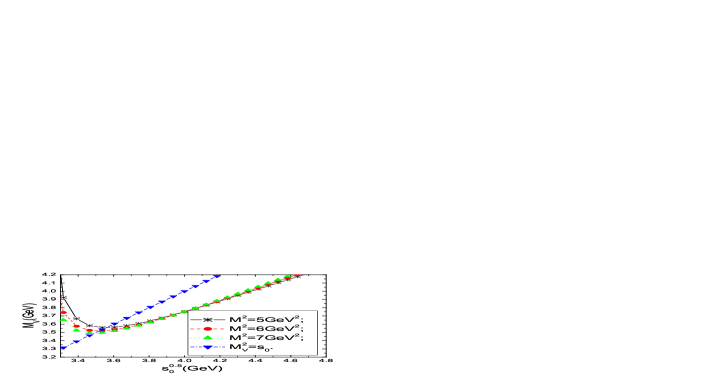
Figure 1: $M_{V}$ with Borel parameter $M^{2}$ and threshold parameter $s_{0}$.

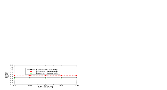
Figure 2: $M_{V}$ with Borel parameter $M^{2}$ from Eq.(16).

Taking into account all the uncertainties, we obtain the value of the mass of the $D_{s}(2700)$, which is shown in Fig.2,

$$M_{V} = (3.75\pm 0.18)\rm{GeV}\,.$$ (18)

It is obvious that our numerical value is larger than the experimental data $M_{V}=2.708\rm{GeV}$, the vector current can interpolate a charmed tetraquark state with the mass about $M_{V}=3.75\rm{GeV}$ or even larger, such tetraquark component should be small in the $D_{s}(2700)$.

If one want to retain the pole dominance of the conventional QCD sum rules, we take the replacement for the weight functions in Eqs.(15-16),

$$\exp\left\{-\frac{s}{M^{2}}\right\} \rightarrow \exp\left\{-\left(\frac{s}{M^{2}}\right)^{2}\right\}\,,$$

$$\exp\left\{-\frac{M_{V}^{2}}{M^{2}}\right\} \rightarrow \exp\left\{-\left(\frac{M_{V}^{2}}{M^{2}}\right)^{2}\right\}\,,$$ (19)

and obtain new QCD sum rules for the mass of the vector tetraquark state.

$$f_{V}^{2}M_{V}^{8}\exp\left\{-\left(\frac{M_{V}^{2}}{M^{2}}\right)^{2}\right\} = \int_{m_{c}^{2}}^{s_{0}}ds\frac{\mbox{Im}\Pi(s)}{\pi}\exp\left\{-\left(\frac{s}{M^{2}}\right)^{2}\right\}\,,$$ (20)

$$M_{V}^{4} = \int_{m_{c}^{2}}^{s_{0}}ds\frac{\mbox{Im}\Pi(s)}{\pi}s^{2}\exp\left\{-\left(\frac{s}{M^{2}}\right)^{2}\right\}/$$ (21)

$$\int_{m_{c}^{2}}^{s_{0}}ds\frac{\mbox{Im}\Pi(s)}{\pi}\exp\left\{-\left(\frac{s}{M^{2}}\right)^{2}\right\}\,,$$

As the main contributions come from the perturbative term, the hadronic spectral density above and below the threshold can be successfully approximated by the perturbative term. If we take typical values for the parameters $\sqrt{s_{0}}=4.0\rm{GeV}$ and $M^{2}=(7-9)\rm{GeV}^{2}$, the contribution from pole term in Eq.(20) is dominating, about $53\%-84\%$. Taking into account all the uncertainties, we obtain the value of the mass of $D_{s}(2700)$, which is shown in Fig.3,

$$M_{V} = (3.71\pm 0.15)\rm{GeV}\,.$$ (22)

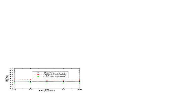
Figure 3: $M_{V}$ with Borel parameter $M^{2}$ from Eq.(21).

4 Conclusion

In this article, we take the point of view that the $D_{s}(2700)$ be a tetraquark state which consists of a scalar diquark and a vector antidiquark, and calculate its mass with the QCD sum rules. The numerical result indicates that the mass of vector charmed tetraquark state is about $M_{V}=(3.75\pm 0.18)\rm{GeV}$ or $M_{V}=(3.71\pm 0.15)\rm{GeV}$, which is about $1\rm{GeV}$ larger than the experimental data. Such tetraquark component should be very small in the $D_{s}(2700)$, the dominating component may be the $c\bar{s}$ state, we can take up the method developed in Ref.[18] to study the mixing between the two-quark component and tetraquark component with the interpolating current $\widehat{J}_{\mu}(x)=cos\theta J_{\mu}(x)+sin\theta\langle\bar{q}q\rangle\bar{s}(x)\gamma_{\mu}c(x)$. The decay $D_{s}(2700)\to D^{0}K^{+}$ can occur mainly through creation of the $u\bar{u}$ pair in the QCD vacuum, we resort to the ${}^{3}P_{0}$ model to calculate the decay width [19], although the ${}^{3}P_{0}$ model is rather crude.

References

[1] J. Brodzicka and H. Palka, et al,
arXiv:0707.3491.
[2] S. Godfrey and N. Isgur, Phys. Rev. D32 (1985) 189;
F. E. Close, C. E. Thomas, O. Lakhina and E. S. Swanson, Phys. Lett.
B647 (2007) 159; D. Ebert, V. O. Galkin and R. N. Faustov,
Phys. Rev. D57 (1998) 5663; Erratum-ibid. D59 (1999)
019902.
[3] K. Abe, et al, hep-ex/0608031.
[4] B. Aubert, et al, Phys. Rev. Lett. 97 (2006) 222001.
[5] M. A. Shifman, A. I. Vainshtein and V. I. Zakharov,
Nucl. Phys. B147 (1979) 385, 448; L. J. Reinders, H.
Rubinstein and S. Yazaki, Phys. Rept. 127 (1985) 1.
[6] S. Narison, QCD Spectral Sum Rules, World Scientific Lecture Notes
in Physics 26 (1989) 1; P. Colangelo and A. Khodjamirian,
hep-ph/0010175.
[7] H. X. Chen, A. Hosaka and S. L. Zhu, Phys. Rev. D74 (2006)
054001; H. X. Chen, A. Hosaka and S. L. Zhu, Phys. Rev. D76
(2007) 094025.
[8] M. Buballa, Phys. Rept. 407 (2005) 205.
[9] T. Schafer, E. V. Shuryak and J. J. M. Verbaarschot, Nucl. Phys. B412 (1994) 143, 1994.
[10]
A. De Rujula, H. Georgi and S. L. Glashow, Phys. Rev. D12
(1975) 147; T. DeGrand, R. L. Jaffe, K. Johnson and J. E. Kiskis,
Phys. Rev. D12 (1975) 2060; T. Schafer and E. V. Shuryak,
Rev. Mod. Phys. 70 (1998) 323.
[11] C. J. Burden, L. Qian, C. D. Roberts, P. C. Tandy and M. J.
Thomson, Phys. Rev. C55 (1997) 2649.
[12] W.-M. Yao, et al, J. Phys. G33 (2006) 1.
[13] Z. G. Wang and S. L. Wan, J. Phys. G34 (2007)
505; Z. G. Wang and S. L. Wan, Nucl. Phys. A778 (2006) 22; Z.
G. Wang and S. L. Wan, Chin. Phys. Lett. 23 (2006) 3208; Z. G.
Wang, Nucl. Phys. A791 (2007) 106.
[14] R. D. Matheus, S. Narison, M. Nielsen and J. M. Richard,
Phys. Rev. D75 (2007) 014005.
[15] S. H. Lee, A. Mihara, F. S. Navarra and M. Nielsen,
arXiv:0710.1029.
[16] B. L. Ioffe, Prog. Part. Nucl. Phys. 56 (2006)
232; and references therein.
[17] R. D. Matheus and S. Narison, hep-ph/0412063;
W. Wei, P. Z. Huang, H. X. Chen and S. L. Zhu,
JHEP 0507 (2005) 015; Z. G. Wang, S. L. Wan and W. M. Yang,
Eur. Phys. J. C45 (2006) 201.
[18] J. Sugiyama, T. Nakamura, N. Ishii, T. Nishikawa and M.
Oka, Phys. Rev. D76 (2007) 114010.
[19] A. Le Yaouanc, L. Oliver, O. Pene and J. C. Raynal, Phys. Rev. D8 (1973)
2223; A. Le Yaouanc, L. Oliver, O. Pene and J.-C. Raynal, Phys. Rev.
D9 (1974) 1415.