A Side of Mercury Not Seen by Mariner 10

Abstract

More than 60,000 images of Mercury were taken at $\sim 29^{\circ}$ elevation during two sunrises, at $\lambda 820$ nm, and through a 1.35 m diameter off-axis aperture on the SOAR telescope. The sharpest resolve $\sim 0\farcs 22$ (160 km) and cover $190-300^{\circ}$ longitude — a swath unseen by the Mariner 10 spacecraft — at complementary phase angles to previous ground-based optical imagery. Our view is comparable to that of the Moon through weak binoculars. Evident are the large crater Mozart shadowed on the terminator, fresh rayed craters, and other albedo features keyed to topography and radar reflectivity, including the putative huge “Basin S” on the limb. Classical bright feature Liguria resolves across the northwest boundary of the Caloris basin into a bright splotch centered on a sharp, 20 km diameter radar crater, and is the brightest feature within a prominent darker “cap” (Hermean feature Solitudo Phoenicis) that covers much of the northern hemisphere between longitudes $140-250^{\circ}$. The cap may result from space weathering that darkens via a magnetically enhanced flux of the solar wind or that reddens low latitudes via high solar insolation.

1. Introduction

The surface of Mercury is a unique record of early times in our solar system. But the small angular size of this planet and especially its proximity in the sky to the Sun limit the clarity of telescopic views. The Hubble Space Telescope can point at Mercury only during “twilight” conditions in Earth shadow, but these observations have never been attempted. Adaptive optics require for wavefront reference the use of natural and artificial guide stars at small airmass whose light would be swamped by the bright sky. In the mid-1970’s, the Mariner 10 spacecraft made detailed observations of surface topography ($1-1.5$ km resolution over a significant area but often at high sun angle), and inferred magnetic field properties during its mostly successful flybys. Because of the 3:2 spin-orbit resonance of Mercury, the same hemisphere was illuminated during all three encounters.

Over the past 30 yr, the other “mystery hemisphere” has been the target of optical and especially radar imaging to learn if large-scale morphological structures such as impact basins and their antipodal effects that were discovered by Mariner have counterparts elsewhere. Radar imagery has covered more than $3/4$ of this hemisphere and has reached $\sim 5$ km resolution (Harmon et al., 2007); sensitive to surface roughness, tilt, and dielectric constant, radar response does not depend on crater diameter. A preliminary stratigraphy of Mercury was developed from the overlap of features in the Mariner images and is keyed to major basin forming events modified by volcanism. Additional major events recorded on the side not imaged by Mariner could alter this sequence substantially.

Mercury is a bright object, so exposures on even modest aperture telescopes can be brief to “freeze” turbulent astronomical seeing. Despite the large zenith distance and bright sky, selection of the sharpest “lucky images” from many (Fried, 1978) can permit use of an aperture large enough to map surface topography. Notable studies of Mercury using this technique mapped longitudes $270-330^{\circ}$ (Baumgardner et al., 2000; Dantowitz et al., 2000) in the morning sky and $210-285^{\circ}$ (Ksanfomality, 2003, 2004) (subsequently expanded and summarized in Ksanfomality & Sprague, 2007) in the evening. Albedo features on Mercury has also been so imaged by Webcam equipped amateur astronomers, with impressive results from modest equipment (F. Melillo, private comm.)

To map the lesser explored quadrant $185-300{}^{\circ}$ in morning illumination (i.e., the complementary phase to that of Ksanfomality & Sprague 2007), in late 2007 March we used a modern high-performance telescope at an excellent observing site, the 4.1 m SOAR telescope atop Cerro Pachon, Chile. In § 2 we describe image acquisition and processing. In § 3 we present our map of this quadrant, and compare to previous optical and radar results. In § 4 we discuss the implications of our findings on the surface properties of Mercury. We summarize in § 5.

2. Methods

2.1. Observing Tactics

2.1.1 Scheduling

Ground-level turbulence can be small at dawn after a night of surface cooling. Our observations were therefore made during a morning elongation of Mercury that was favorable from Chile and that presented to us the hemisphere not mapped by Mariner. Mercury rotates slowly so most longitude coverage during an elongation arises from changes in phase angle. During the second half of the 2007 March-April elongation Mercury spanned $7\farcs 2-6\farcs 4$ as its phase increased from 55 to $67\%$ and sub-Earth longitude increased from $178^{\circ}$ to $222^{\circ}$, while the sub-Earth latitude was $\sim-3.5^{\circ}$. We intended to observe on 4 mornings every 3 days starting at maximum elongation, during pre-scheduled University of North Carolina (UNC) and engineering time. Unfortunately, weather delivered a sequence of excessive humidity, clouds, and bad seeing, so we obtained data only on the mornings of 2007 March 23 and April 1. To calibrate, we also observed stars, Jupiter, and Saturn.

The SOAR telescope is often operated remotely from partner institutions over the Abeline (Internet2) network (Cecil & Crain, 2004), sharing with other Cerro-Tololo Inter-American Observatory (CTIO) telescopes up to 35 Mbit s^-1 bandwidth. Multiple instruments are installed for the long-term at various SOAR foci. Our telepresence during dawn and sunrise had minimal impact on other programs. Because our observations ended after sunrise, certain detector calibrations that would ideally be done with dawn illumination were instead made either during evenings or within the light-tight dome.

2.1.2 Preparing and operating the telescope

Most modern telescopes mount instruments at Nasmyth foci where it is particularly challenging to baffle light scatter. Thus, we did not expect to observe beyond sunrise over the Andes east of Cerro Pachon. Also, the tertiary and primary telescope mirrors look upward so are easily contaminated with light scattering dust. Luckily, the SOAR optics had been washed thoroughly $\sim 10$ days before our observations began.

To obtain sharp images from a stack of tens of thousands of exposures in seeing characterized by spatial scale $r_{0}$, one must reduce the telescope aperture $D$ until $D/r_{0}\sim 9$ (Fried, 1978). $r_{0}$ degrades with zenith angle $z$ and wavelength as $(500\,\mbox{nm}/\lambda)^{1.2}\cos^{-0.6}z,\approx 1$ for our study of Mercury. We fabricated and installed across the top ring of the telescope near the entrance pupil an opaque, black cloth mask. The mask required an hour to install beginning at the start of astronomical twilight. Hoping for better than average seeing at a challenging $\sim 27^{\circ}$ elevation, we had our tailor cut an elliptical hole of minor diameter 1.35 m. This projected a circular pupil, unobstructed by telescope secondary mirror “spider” supports.

The mask blocked the facility Shack-Hartmann array from sampling the full set of stellar wavefront tilts to set telescope active optics, normally done after large-angle motions. The software could not handle an off-axis sub-aperture. We therefore used only pre-calibrated lookup tables, indexed exclusively by temperature sensors and the telescope elevation angle. We set up on a star at $\sim 30^{\circ}$ elevation to confirm focus and pointing, and to make a movie to understand the current speckle structure. On the first morning, 2007 March 23, long exposure seeing scaled to the zenith was $\sim 0\farcs 6$, and through our aperture we saw what we had hoped to see: a small number of gyrating speckles of comparable brightness that occasionally merged to produce a very sharp image. A larger aperture would have passed more speckles, yielding far fewer coincidences hence sharp images. We could see clear astigmatism on either side of nominal focus, indicating incomplete setting of the telescope active optics. However, because our target was centered and only a few arc-seconds across, astigmatism was useful to maintain accurate focus so we did not null it. The 2007 April 1 seeing was worse and we obtained fewer but still excellent images on occasion, probably because the higher sun angle on the disk enhanced the contrast of Mercury’s subtle shadings.

We acquired Mercury at $15^{\circ}$ elevation, SOAR’s limit. These images were horrible, of course, but improved steadily as sunrise approached. We recorded occasional crisp detail between $26$ and $30^{\circ}$ elevation before scattered light overwhelmed the signal as the Sun crested the Andes.

2.1.3 Camera selection and operation

We used an Andor Corporation Luca model camera, a thermoelectrically cooled (stabilized to $-20^{\circ}$C), non-evacuated housing of a Texas Instruments frame-transfer (electronic shutter) $658\times 496$ array of 10 micron square pixels and $\sim 18\%$ QE at $\lambda 820$ nm. The camera records 30 full-frames s^-1 with nominal 25 electrons rms readout noise. With a typical acquisition window of $140\times 130$ $2\times 2$ binned pixels (each $0\farcs 06$ on the sky), we acquired 140 frames s^-1. The camera was connected without reduction optics directly to a telescope Nasymth focus and to a PC that used Andor’s SOLIS program to acquire data to a SATA drive (49 Mbyte s^-1 transfer speed). A feature of this camera is its electron multiplying gain, adjustable by software to set the amplification of a separate “gain register” prior to readout. With minimal amplification, exposures of $6.5-8.7$ ms produced peak counts $\sim 1/4$ of the camera’s 14-bit digitization range and had negligible readout noise. We used this setting for all observations and calibrations because we hoped to work as late as feasible into daylight without saturating the detector on the brightening sky. To reduce atmospheric dispersion below one resolution element, we used a $\lambda 95$ nm wide interference filter from CTIO’s collection, centered at $\lambda 820$ nm, and operating in the effective f/38 beam.

We took multiple strings of 10,000 exposures stored as $300-400$ Mbyte FITS format datacubes. A VNC connection from our remote observing room in Chapel Hill to the computer desktop in Chile allowed us to control data acquisition and to review representative frames with ds9. We used the simple bbcp program to deliver data expeditiously to UNC at 3 Mbyte s^-1 (while maintaining the VNC connection, an audio/video link to the telescope operator, and telescope/site telemetry). During each dawn we recorded and transferred $\sim 5$ Gbyte of data into UNC’s SOAR archive.

We also recorded stacks of 10,000 dark frames of the same duration as the data, exposures so short that they showed only fixed pattern noise near the readout, a 6 DN top-to-bottom gradient in the electronic bias level, and several tens of “hot pixels”. We subtracted the average dark from each exposure of the datacube.

Although we recorded evening sky flats and morning dome flats, these unfortunately failed to remove spots in data frames, especially the March 23 data. Spots seem to arise from contamination on the CCD surface, not on its dewar window, so are sensitive to details of their specific illumination. They are noticeable when successive exposures are viewed as a movie; the dancing planet image is seemingly being viewed through a somewhat dirty window. Their effect is smeared across the final stacked image by planet motions between its constituent exposures, but image contrast on March 23 would have been higher, and confidence in the reality of subtle albedo variations and shadowing near the terminator increased, without it. It was also unclear if the nominal flats calibrated pixel-to-pixel sensitivity variations. To better match illumination to reduce problems in the flat fields associated with scattered light from bright dome or sky, we resorted to using the disks of Jupiter and Saturn. We obtained 1,000 to 10,000 exposure datacubes of these planets through the filter. The 200 ms Jupiter exposures showed often exquisite detail in the cloud belts around, for example, the Little Red Spot, unsurprising given that this planet was imaged near the zenith in reasonably good seeing. We coadded the worst $10\%$ of the images that were further blurred by motion between frames, and then used the IRAF fit1d task to produce spline3 fits row by row and column by column. We combined row and column fits and ratioed the result into the original image to obtain a flat field. We scaled the flat to obtain best results and divided it into each exposure of the datacube. We retained for further processing the $40,000$ highest elevation images from the first morning and $20,000$ from the last.

2.2. Selecting and Processing Sharp Frames

Key to lucky imaging is how one finds the needle in the haystack. After exploring and rejecting contrast and wavelet based algorithms, we simply selected by eye the best image of $\sim 500$ from the highest-elevation string, and then automatically cross-correlated this with the other tens of thousands to produce an output sequence sorted from narrowest $50\%$ waist of the two-dimensional correlation peak to fuzziest. Ranking excluded all double exposures caused by paired clumps of speckles, and most of the images with fuzzy limbs or gross distortions. Some images deemed acceptable were in fact distorted (“looming”), rotated, or blurred over part of their area. These were rejected in the next step after we had loaded the nominally best 500 from the combined stack of all strings into the RegiStax program (widely used by amateur astronomers to stack Webcam images) to refine the cross-correlation, and hence rerank, images within a $128\times 128$ pixel box that spanned the planet.

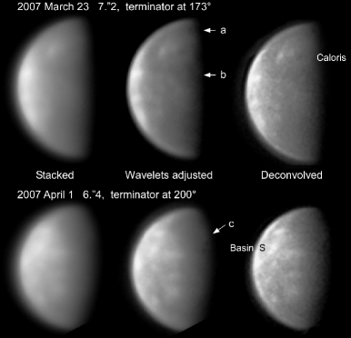
We selected the final set of images in this sorted sequence of $\sim 60$ by eye, drizzle stacking the best 20 and 13 frames from the first and second mornings, respectively, to form high signal-to-noise ratio final images with $0\farcs 03$ pixels (Fig. 1, left images). After setting the scale of wavelet number 1 to encompass noise, we attenuated its amplitude while boosting wavelet scales $2-4$. The result (Fig. 1, middle images) equaled our expectations from a blurred, $0\farcs 2$ FWHM version of a Mariner full disk image. As an alternative to wavelets, we used the smart sharpening filter in Photoshop CS3 followed by $50-100$ iterations of Richardson-Lucy deconvolution (Fig. 1, right images, Richardson 1972) to further sharpen bright features but now non-uniquely and with some added noise. We did not dig out features along the terminator beyond those immediately apparent (Fig. 1, arrows) because this would have required a much larger final image stack to attain resolution above the Rayleigh limit (Ksanfomality & Sprague, 2007), and because topography within $15^{\circ}$ of the March 23 terminator had been mapped by Mariner.

We drew a circle around the planet image of the correct radial scale and found its center to $\pm 0.5$ pixel. To reduce the phase-dependent planetary illumination to map albedo variations, we weighted image intensities by multiplicative factor $[\cos\phi\bullet\max(0.3,\left|\sin\theta\right|)]^{k}$ with $\phi$ the latitude and $\theta$ the longitude difference from the terminator to the location on the planet and $k=-1/2$ selected unphysically simply to improve appearances.

3. Empirical Results

Projecting the two enhanced final images made Figure 2$a$, a cylindrical-equidistant map. Between longitudes $180-300^{\circ}$, we locate features to better than $2^{\circ}$ near the planetary equator and to within $3^{\circ}$ near the top of the map, these uncertainties arising from inexact centers of the half or gibbous shapes of the planet.

Figure 1.— SOAR telescope views of a side of Mercury not imaged by Mariner 10. Left: Composites of the sharpest exposures (top, 20 of 40,000 acquired at $29-30^{\circ}$ elevation; bottom, 13 of 20,000 at $25-27^{\circ}$ elevation). They contain much detail that we have attempted to enhance (middle) by boosting the contribution of intermediate-scale wavelets, or (right) by applying an adaptive sharpening filter followed by $50-100$ iterations of Richardson-Lucy deconvolution with a plausible PSF. Three isolated bright features near the left limb in the top row have rotated to disk center in the bottom where they are revealed in the right column and after correlation with radar images (Harmon et al., 2007) to be rayed craters. Two large basins are labeled on the limbs of the right images: the Caloris basin and putative “Basin S” proposed by Ksanfomality & Sprague (2007). Arrows point to terminator topography discussed briefly in the text.

Figure 2.— (a) Map of uncalibrated $\lambda 820$ nm albedo variations in cylindrical equidistant projection, constructed from the two wavelet adjusted SOAR images (Fig. 1). The Caloris basin and putative Basin S are denoted by broken circles. Bright ramparts of crater Mozart are also evident along the terminator below Caloris (arrows). Crater diameters (from radar images in Harmon et al. (2007)) are shown in km. (b-e) show radar images (Opposite-polarization component unless labeled SC for Same component) of craters that coincide with our bright features. Radar data are ambiguous across the dark Doppler equators in (b) and (c). However, albedo patterns in our data allow us to identify the circled features of pairs in panel (c) as spurious.

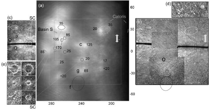
Our albedo map agrees with the fuzzier but color-calibrated one of Warell & Limaye (2001) from the 0.5 m Swedish Vacuum Telescope used during daylight closer to the zenith. Figure 3 places our map in the context of a mosaic of published Arecibo radar images (Harmon et al., 2007), and we highlight some agreements below. Correlating images at these two frequencies is not trivial. As Harmon et al. (2007) noted, radar images whose polarization is opposite to the transmitted beam are sensitive to sharp surface relief, not shallow gradients, while same-polarization images respond mostly to wavelength-scale surface roughness and somewhat to variations of surface dielectric properties. Both image types are ambiguous across the Doppler equator, but the spurious feature can be rejected by comparing to other radar scans at different sub-Earth latitude or, as we show below, to our images.

We tried to compare our map to the crescent image analyzed by Ksanfomality & Sprague (2007), which overlaps somewhat with our images but has opposite illumination and foreshortening. What they saw on the bright limb would be evident in the middle of our April 1 image. The brightest feature in their image, at $(235^{\circ},+32^{\circ})$, is undetected in ours. Their bright feature at $(247^{\circ},-7^{\circ})$ may be associated with ours at $(240^{\circ},-10^{\circ})$. Their crater at $(270^{\circ},-15^{\circ})$ is our feature “l”. Unfortunately, further comparison is unfeasible given the rapid change in brightness of topographic features as sun angles vary, and the amplification of the CCD contamination in our March 23 image that would result from the extensive image processing required to super-resolve details beyond the telescope-aperture Rayleigh limit.

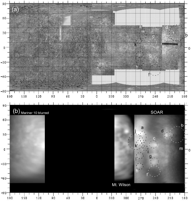
Figures 2 and 3 reveal albedo variations tied to radar rayed craters and large dark areas. For example, dark region “j” in Figure 3$b$ centered at $(\sim 280^{\circ},+16^{\circ})$ is the huge “Basin S” posited by Ksanfomality & Sprague (2007). To its south and east lie bright radar craters. Feature “c” in panel Figure 2$a$ is a 125 km diameter crater that Harmon et al. (2007) note as asymmetrically brightened to the north; instead, we see an east-west extension of its bright material. Bright features “a” in Figure 3 form a broken ring of what radar image Figure 2$a$ shows are rayed craters hence must be fresher than an ancient Basin S. These are clearly not the encircling basin ramparts that Ksanfomality (2004) saw shadowed at lower sun angle. Indeed, Harmon et al. (2007) found radar highlighting only on the western side of the basin, beyond the limb to us. Bright regions are evident along the rest of Basin S in the Baumgardner et al. (2000) plus Dantowitz et al. (2000) composite Mount Wilson image in the middle of Figure 3.

Eastward at longitudes $242-250^{\circ}$, prominent bright clumps at latitudes $+10,-10$, and $-28^{\circ}$ are all radar craters. In our sharpest images (and Fig. 1 right images), each is a bright core surrounded by a slightly fainter splotch. In extent, they all are comparable to the largest crater ray systems imaged at high sun angle by Mariner on the opposite hemisphere (Fig. 3$b$ left).

Figure 3.— Montage of some previous maps of Mercury and our data, cylindrical equidistant projection. (a) Mariner 10 photo map at left, at right is a mosaic of Arecibo radar images with a few showing north-south Doppler ambiguities (Harmon et al., 2007); (b) A Mariner mosaic blurred to our resolution at left, Ksanfomality (2004)’s combination of the Baumgardner et al. (2000) and Dantowitz et al. (2000) Mount Wilson images in the middle, and at right our SOAR data. Labeled features are discussed in the text.

Feature “g” in Figure 2$a$ is 200 km across and seems to have radial striations, with Figure 2$c$ showing a crisp radar crater of diameter 85 km with central peak and a muted crater more than twice as wide immediately to the south. Further south still in our images in Figures 2$a$ and 3$b$ is dark region “f” centered at $(240^{\circ},-45^{\circ})$, Solitudo Persephones in the Dollfus et al. (1978) IAU albedo map. Comparable in size to the Caloris basin, “f” is not surrounded by radar or optical bright features, so is perhaps a plain not a large impact basin with substantial ramparts. Is it connected physically to “g”?

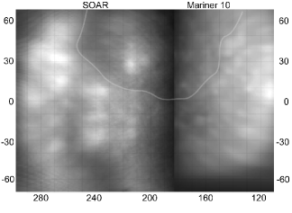
The right (eastern) side of our map spans the Mariner unimaged western boundary of the Caloris basin, “b” in Figure 3. Its floor seems to be composed of multiple dark regions. But, intriguingly, an only slightly brighter but still dark area extends far beyond Caloris, poleward in a diagonal swath from $(190^{\circ},+5^{\circ})$ to $(260^{\circ},+45^{\circ})$; this is the classical Hermean albedo feature Solitudo Phoenicis in the IAU map (Dollfus et al., 1978). In fact, despite the lack of photometric calibration, the Mariner mosaic Figure 4 (right) shows that this high-latitude darkening continues eastward to longitude $140^{\circ}$.

Comparing Figure 2$a$ and $c$, we see that the dark area sometimes coincides with a change in radar surface texture and has a sharp radar boundary between $240-250^{\circ}$. The dark region seems to be devoid of prominent rayed craters, implying relatively recent origin, with a striking exception: bright “island d” in Figure 3 spans $\sim 15{}^{\circ}$ (350 km) at the end of slightly dimmer IAU Hermean region Liguria (Dollfus et al., 1978). The closest radar feature in Figure 2$d$ is a fresh crater at $(203^{\circ},+30^{\circ})$, which is, however, several degrees east of our eastern feature. The optically much brighter western feature at $(217^{\circ},+28^{\circ})$ is an inconspicuous 20 km diameter radar crater that seems to sit on a larger degraded crater (Fig. 2d); its lack of correlation with a prominent radar crater is similar to the situation for the brightest feature in the Mount Wilson images (Fig. 3, middle). On April 1 “d” lay only $17^{\circ}$ from the terminator, yet was still so bright that it appears in Figure 1 to protrude into the shadowed area (arrow “c”). We propose the name “Mistral” for the sharp, optically bright 20 km diameter crater at $(217^{\circ},+28^{\circ})$.

In our March 23 image, another dark region, Solitudo Atlantis (Dollfus et al., 1978), is evident to the south and east, and is bounded to the west by isolated rayed craters near $210^{\circ}$. This region is mottled, indicating its incipient resolution into partially shadowed craters. Indeed, the illuminated western ramparts of the large crater Mozart are just detectable (arrow “b”) in Figure 1. Finally, dark patch “a” $(190^{\circ},+63^{\circ})$ near the terminator in Figure 2 is a region without published radar data.

4. Discussion

4.1. “Basin S”

Ksanfomality (2004) discovered and argued for this huge (“Skinakas”) basin, centering it at $(280^{\circ},+8^{\circ})$, $\sim 5^{\circ}$ south of our estimate (which, being at the limb, is less accurate). Both halves appear near the terminator in the images of Baumgardner et al. (2000); Dantowitz et al. (2000) and Ksanfomality (2003), respectively, and make it comparable in size to Caloris. It may be bigger: Ksanfomality (2004) showed that the intensity cut across the middle of this structure is consistent with two concentric rings of ramparts that extend into the quadrant that we observed on April 1. Exceeding in extent the lunar south pole-Aitken feature, if a true impact structure it would be one of the largest basins in the solar system. The formation of Caloris was the culminating event in the Mariner derived stratigraphy of Mercury. Ksanfomality & Sprague (2007) assert that Basin S has a degraded appearance, implying that it is older than Caloris. The ejecta deposits of Basin S would probably not extend far enough to over/underlap those from Caloris (permitting direct relative dating from MESSENGER spacecraft imagery during its 2008 gravity-assist flybys of Mercury).

In our April 1 image, Basin S is centered near the bright limb. Within it, radar shows (Fig. 3$a$) a few intermediate size craters and indeed we see a bright one, “k”, that may be what Ksanfomality (2004) attributed as its central peak (which would be an impact signature). But the northern half of Basin S is certainly dark even at high sun angle, and is surrounded on its visible south and east sides by bright craters, for example, “a”. In fact, radar craters account for all the optical bright spots; there are no signs of boundary ramparts on the E side visible to us. To the west beyond our limb, Harmon et al. (2007) find radar highlights and speculate that these may be the inner western rim of Basin S. There is no sign in the Mariner imagery of hilly “weird terrain” at the putative Basin S antipode as is the case for Caloris.

4.2. Other dark features

As mentioned in § 3, a dark swath in the 2007 March 23 image extends westward at reduced prominence in the April 1 image and eastward in the Mariner mosaic (Fig. 4). The boundary between lower and higher albedo regions is sharp, as is the boundary of the “island” of bright features “d”. The radar image Figure 2$c$ also shows a sharp boundary, but only between $240-250^{\circ}$ does it coincide with the albedo change. The darker “cap” is a striking asymmetry across Mercury; there are indications of a counterpart darkening at high southern latitudes in Figure 3$b$. Is it superficial, a result of space weathering that darkens and/or reddens an exposed surface? We have only monochrome red images, so cannot map colors. One way to darken the surface is an enhanced influx of charged particles near the magnetic poles (Killen et al., 2001), although Mercury’s field is supposed to be strong enough to keep the solar wind from reaching the surface most of the time (Russell et al., 1988). Alternatively, equatorial and lower latitude regions could be reddened (hence brightened in our filter) relative to the poles by weathering from enhanced solar irradiation (Hapke, 2001). If the darkening is instead due to a fundamental change in surface properties (as suggested by the change in radar texture), this asymmetry would cause Mercury to resemble the other terrestrial planets.

Figure 4.— Right: Blurred Mariner 10 mosaic image; left: SOAR map, where the $\cos\theta$ (with $\theta$ the angle to the sun from the vertical at each point on the planet’s surface) illumination pattern has been removed. Outlined at top is the approximate extent of the darker region that extends poleward from northern mid-latitudes over this hemisphere.

4.3. Volcanoes?

How volcanism may have shaped the planet’s surface is controversial. No definitive volcanic feature was identified even in Mariner 10 close-ups. A non-Lunar aspect is the extensive distribution of inter-crater plains, attributed to either volcanism or obscuring basin ejecta. Robinson and Lucey (1997) attempted to calibrate the compromised Mariner 10 two-filter photometry, and have compared the resulting color variations to lunar measurements. In their view, changes in surface color are due both to space weathering and to intrinsic compositional variations consistent with volcanic fire fountains.

Long-term volcanism is a possibility following the radar measurements by Margot et al. (2007) of variations in the planet’s forced longitudinal libration that are consistent with mantle slippage inertia over a partially molten core. Such a core structure also explains the weak magnetic field discovered by Mariner. (Alternatively, Ksanfomality & Sprague 2007 noted that Mariner 10 passed over Basin S, and posit that the measured field is a relic of this putative impact.) The absence of global tectonics other than the overall contraction inferred from planet-wide scarps (Strom et al., 1975) may permit substantial volcanic structures to accumulate slowly over time, not just as fire fountains in the distant past. Shield volcanoes could be flat enough to be subtle in existing radar images that are sensitive only to short-wavelength tilts; radar altimetry (Clark et al., 1988) has not spanned large areas of the planet. Nevertheless, all bright features in our map can be attributed to rays or ramparts of radar craters.

5. Summary

Our “lucky image” stacks bettered $0\farcs 25$ resolution and have mapped prominent rayed craters and other features across part of the hemisphere unseen by Mariner 10 but subsequently imaged by radar. The region complements that studied by Ksanfomality & Sprague (2007) also using short exposure stacks. They and Ksanfomality (2004) have posited a large dark feature (“Basin S” or “Skinakas basin”) near $(280^{\circ},+10^{\circ})$. Although we observed it near the limb, we do see its darker floor even at the high sun angle that brightens some adjacent craters. However, we find only bright radar craters around it, and no features that could be attributed to basin ramparts on its eastern boundary.

Several topographic features are observed at the terminator, including ramparts of the large crater Mozart. A very bright spot that is a sharp radar crater lies within a dark swath that extends across at least $140-250^{\circ}$ longitude at latitudes reaching northward of $30^{\circ}$ at $180^{\circ}$ longitude to northward of $+45^{\circ}$ latitude at $250^{\circ}$. No other prominent rayed craters, even at higher sun angles, lie within this region. Starting in 2011, MESSENGER’s intensive mapping of compositional variations and topography as it orbits will bring Mercury’s history into ever sharpening focus, and hopefully will require no luck whatsoever.

References

- Baumgardner et al. (2000) Baumgardner, J., Mendillo, M., & Wilson, J. K. 2000, AJ, 119, 2458
- Cecil & Crain (2004) Cecil, G. & Crain, A. C. 2004, Proceedings of the SPIE, 5493, 73
- Clark et al. (1988) Clark, P. E., Leake, M. A., & Jurgens, R. F. 1988, in Mercury, ed. F. Vilas et al. (Tucson: University of Arizona Press), 77
- Dantowitz et al. (2000) Dantowitz, R. F., Teare, S. W., & Kozubal, M. J. 2000, AJ, 119, 2455
- Dollfus et al. (1978) Dollfus, A., Chapman, R., Davies, M. E., Gingerich, O., Goldstein, R., Guest, J., Morrison D., & Smith, B. A. 1978, Icarus, 34, 210
- Fried (1978) Fried, D. L. 1978, J. Opt. Soc. Am., 68, 1651
- Hapke (2001) Hapke, B. 2001, J. Geophys. Res., 108, 10039
- Harmon et al. (2007) Harmon, J. K., Slade, M. A., Butler, B. J., Head, J. W., Rice, M. S., & Campbell, D. B. 2007, Icarus, 187, 374
- Killen et al. (2001) Killen, R. M., Potter, A. E., Reiff, P., Sarantos, M., Jackson, B. V., Hick, P., & Giles, B. 2001, J. Geophys. Res., 106, 20509
- Ksanfomality (2003) Ksanfomality, L. V. 2003, Solar System Research, 37, 469
- Ksanfomality (2004) Ksanfomality, L. V. 2004, Solar System Research, 38, 21
- Ksanfomality & Sprague (2007) Ksanfomality, L. V. & Sprague, A. L. 2007, Icarus, 188, 271
- Margot et al. (2007) Margot, J.-L., Peale, S., Jurgens, R. F., Slade, M. A., & Holin, I. V. 2007, Science, 316, 710
- Richardson (1972) Richardson, W. H. 1972, J. Opt. Soc. Am., 62, 55
- Robinson and Lucey (1997) Robinson M S & Lucey P G 1997, Science, 275, 197
- Russell et al. (1988) Russell, C. T., Baker, D. N., & Slavin, J. A. 1988, in Mercury, ed. F. Vilas et al. (Tucson: University of Arizona Press), 514
- Strom et al. (1975) Strom, R. G., Trask, N. J., & Guest, J. E. 1975, J. Geophys. Res., 80, 2478
- Warell & Limaye (2001) Warell, J. & Limaye, S. S. 2001, Planet. Space Sci., 49, 1531