Gamma-ray and neutrino diffuse emissions of the Galaxy above the TeV

Abstract

In this contribution we will discuss recent results concerning the intensity and the angular distribution of the gamma-ray and neutrino emissions as should be originated from the hadronic scattering of cosmic rays (CR) with the interstellar medium (ISM). We assumed that CR sources are supernova remnants (SNR) and estimated the spatial distribution of primary nuclei by solving numerically the diffusion equation. For the ISM, we considered recent models for the 3D spatial distributions of molecular hydrogen. Respect to previous results, we find the secondary gamma-ray and neutrino emissions to be more peaked along the galactic equator and in the galactic centre which improves significantly the perspectives of a positive detection. We compare our predictions with the experimental limits/observations by MILAGRO and TIBET (for the gamma-rays) and by AMANDA-II (for the neutrinos) and discuss the detection perspectives for a km3 neutrino telescope to be built in the North hemisphere.

1 Introduction

Several orbital observatories (see [3] for a review), especially EGRET [16, 8], found that, at least up to $10~{}{\rm GeV}$, the Galaxy is pervaded by a $\gamma$-ray diffuse radiation. While a minor component of that emission is likely to be originated by unresolved point-like sources, the dominant contribution is expected to come from the interaction of galactic cosmic rays (CR) with the interstellar medium (ISM). Since the spectrum of galactic CR extends up to the EeV, the spectrum of $\gamma$-ray diffuse galactic emission should continue well above the energy range probed by EGRET. That will be soon probed by GLAST [13] up to $~{}300~{}{\rm GeV}$ and by air shower arrays (ASA) (e.g. MILAGRO [19, 18] and TIBET [12]) above the TeV.

Above the GeV, the main $\gamma$-ray emission processes are expected to be the decay of $\pi^{0}$ produced by the scattering of CR nuclei onto the diffuse gas (hadronic emission) and the Inverse Compton (IC) emission of relativistic electron colliding onto the interstellar radiation field (leptonic emission). It is unknown, however, what are the relative contributions of those two processes and how they change with the energy and the position in the sky (this is so called hadronic-leptonic degenerary). Several numerical simulations have been performed in order to interpret EGRET as well as forthcoming measurements at high energy (see e.g. [2, 1, 21] ). Generally, those simulations predict the hadronic emission to be dominating between 0.1 GeV and few TeV, while between 1 and 100 TeV a comparable, or even larger IC contribution may be allowed.

The 1-100 TeV energy range, on which we focus here, is also interesting from the point of view of neutrino astrophysics. In that energy window neutrino telescopes (NTs) can look for up-going muon neutrino and reconstruct their arrival direction with an angular resolution better than $1^{\circ}$. Since hadronic scattering give rise to $\gamma$-rays and neutrinos in a known ratio, the possible measurement of the neutrino emission from the Galactic Plane (GP) may allow to get rid of the hadronic-leptonic degeneracy.

In this contribution we discuss the main results of a recent work were we modelled the $\gamma$-ray and neutrino diffuse emission of the Galaxy due to hadronic scattering [9]. Our work improves previous analysis under several aspects which concern the distribution of CR sources; the way we treated CR diffusion by accounting for spatial variations of the diffusion coefficients; the distribution of the atomic and molecular hydrogen.

2 The spatial structure of the ISM

In order to assess the problem of the propagation of CRs and their interaction with the ISM we need the knowledge of three basic physical inputs, namely: the distribution of SuperNova Remnants (SNR) which we assume to trace that of CR sources; the properties of the Galactic Magnetic Field (GMF) in which the propagation occurs; the distribution of the diffuse gas providing the target for the production of $\gamma$-rays and neutrinos through hadronic interactions. In the following we assume cylindrical symmetry and adopt the Sun galactocentric distance $r_{\odot}=8.5~{}{\rm kpc}$.

2.1 The SNR distribution in Galaxy

Several methods to determined the SNR distribution in the Galaxy are discussed in the literature (see e.g. that based on the surface brightness - distance relation [6]). Here we adopt a SNR distribution a distribution as inferred from observations of related objects, such as pulsars or progenitor stars, as done e.g. in [11] which is less plagued from sistematics and agrees with that inferred from the distribution of radioactive nuclides like of ²⁶Al . A similar approach was followed in [22] where, however, the contribution of type I-a SNR (which is dominating in the inner 1 kpc) was disregarded.

2.2 Regular and random magnetic fields

The Milky Way, as well as other spiral galaxies, is known to be permeated by large-scale, so called regular, magnetic fields as well as by a random, or turbulent, component. The orientation and strength of the regular field is measured mainly by means of Faraday Rotation Measurements (RMs) of polarised radio sources. From those observations it is known that the regular field in the disk of the Galaxy is prevalently oriented along the GP. Following [14, 15] we adopt the following analytical distribution for the disk and the halo:

$$B_{\rm reg}(r,z)=B_{0}\exp\left\{-\frac{r-r_{\odot}}{r_{B}}\right\}\;\frac{1}{2\cosh(z/z_{r})}~{},$$ (1)

where $B_{o}\equiv B^{\rm disk}_{\rm reg}(r_{\odot},0)\simeq 2~{}\mu{\rm G}$ is the strength at the Sun circle. The parameters $r_{B}$ and $z_{r}$ are poorly known. However we found that our final results are practically independent on their choice. In the following we adopted $r_{B}=8.5~{}{\rm kpc}$ and $z_{r}=1.5~{}{\rm kpc}$.

More uncertain are the properties of the turbulent component of the GMF. Here we assume that it strength follows the behaviour

$$B_{\rm ran}(r,z)=\sigma(r)\;B_{\rm reg}(r,0)\;\frac{1}{2\cosh(z/z_{t})}\;.$$ (2)

where $\sigma(r)$ parematrise the turbulence strength. Here we assume $z_{t}=3~{}{\rm kpc}$. From polarimetric measurements and RMs is known GMF are chaotic on all scales below $L_{\rm max}\sim 100~{}{\rm pc}$. The power spectrum of the those fluctuations is also poorly known. In [9] we considered both a Kolmogorov ($B^{2}(k)\propto k^{-5/3}$) and a Kraichnan ($B^{2}(k)\propto k^{-3/2}$) power spectra.

2.3 The gas distribution

The model which consider here is based on a suitable combination of different analyses which have been separately performed for the disk and the galactic bulge. For the ${\rm H}_{2}$ and HI distributions in the bulge we use a detailed 3D model recently developed by Ferriere et al. [10] on the basis of several observations. For the molecular hydrogen in the disk we use the well known Bronfman’s et al. model [4]. For the HI distribution in the disk, we adopt Wolfire et al. [23] 2-dimensional model. In the following we will assume that helium is distributed in the same way of hydrogen nuclei.

3 CR diffusion

The ISM is a turbulent magneto-hydro-dynamic (MHD) environment. Since the Larmor radius of high energy nuclei is smaller than $L_{\rm max}$, the propagation of those particles takes place in the spatial diffusion regime. The diffusion equation describing such a propagation is (see e.g. [20])

$$-\nabla_{i}\left(D_{ij}(r,z)\nabla_{j}N(E,r,z)\right)=Q(E,r,z)$$ (3)

where $N(E,r,z)$ is the differential CR density averaged over a scale larger than $L_{\rm max}$, $Q(E,r,z)$ is the CR source term and $D_{ij}(E,r,z)$ are the spatial components of the diffusion tensor. In the energy range considered in our work energy loss/gain can be safely neglected. Since we assume cylindrical symmetry the only physically relevant components of the diffusion coefficients are $D_{\perp}$ and $D_{A}$, respectively the diffusion coefficient in the direction perpendicular to ${\bf B}_{\rm reg}$ and the antisymmetric (Hall) coefficient. We adopted expressions for those coefficients as derived by Montecarlo simulation of charged particle propagation in turbulent magnetic fields [5]. Respect to other works, where only isotropic diffusion was considered and a a mean value of the diffusion coefficient was estimated from the observed secondary/primary ratio of CR nuclear species (see e.g. [21]), our approach offers the advantage to provide the diffusion coefficients point-by-point at any energy. We solved the diffusion equation using the Crank-Nicholson method by imposing $N(E)=0$ at the edge of the MF turbulent halo and by requiring that it matches the observed CR spectra at the Earth position for most abundant nuclear species.

4 Mapping the $\gamma$-ray and $\nu$ emission

Under the assumption that the primary CR spectrum is a power-law and that the differential cross-section follows a scaling behaviour (which is well justified at the energies considered in this paper), the $\gamma$-ray (muon neutrino) emissivity due to hadronic scattering can be written as

$$\frac{dn_{\gamma~{}(\nu)}(E;~{}b,l)}{dE} \simeq f_{N}~{}\sigma_{pp}\;Y_{\gamma}(\alpha)$$

$$\int{\rm d}s\;I_{p}(E_{p};~{}r,z)~{}n_{H}(r,z)$$

Here $I_{p}(E_{p};~{}r,z)$ is the proton CR differential flux at the position $r,z$ as determined by solving the diffusion equation; $\sigma_{pp}$ is the $pp$ cross-section; $Y_{\gamma}\simeq 0.04$ and $Y_{\nu_{\mu}+{\bar{\nu}}_{\mu}}\simeq 0.01$ are the $\gamma$-ray and muon neutrino yields respectively as obtained for a proton spectral slope $\alpha=2.7$ (see Fig. 7 in [9, 7] and ref.s therein); the factor $f_{N}\simeq 1.4$ represents the contribution from all other nuclear species both in the CR and the ISM; $s$ is the distance from the Earth; $b$ and $l$ are the galactic latitude and longitude. Here we assume that the slope of the CR injection spectrum is 2.2 and that the GMF turbulent spectrum has a Kraichnan spectrum. Fluxes obtained by using different spatial structure and spectra of the turbulent magnetic field differ by a factor 2 at most. In 1 we compare our results with those obtained in [2].

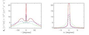
Figure 1: The $\gamma$-ray flux profiles along the GP (left panel) and along $l=0$ (right panel) for $E>1~{}{\rm TeV}$, averaged over $1^{\circ}\times 1^{\circ}$ angular bins. The continuos (red), dot-dashed (blue) and dashed (green) curves correspond respectively to: our work, a model with the same gas density distribution but a uniform CR flux, taken to match direct observations at the Earth; the model considered in [2]. The corresponding neutrino flux can be obtained by dividing this diagram by 3.1.

5 Discussion

First of all, we compare our results with EGRET observations in the $4-10~{}{\rm GeV}$ energy range [8]. That is possible since, already for $<10~{}{\rm TeV}$, nuclei propagation takes place deep into the spatial diffusion regime so that the behaviour of the diffusion coefficients do not change going to lower energies and our results can be safely extrapolated. As we showed in [9], our predictions are in good agreement with EGRET measurements along the GP, but a small deficit which can be easily explained in terms of IC. Then we can reliably compare our results with measurements performed above the TeV with air shower arrays (see Tab. 1) and NTs. We found that with the exception of Cygnus (where one or more sources are likely to increase the local CR density) in all other regions we predict fluxes which are significantly below the experimental limits.

Concerning neutrinos, the only available upper limit on the neutrino flux from the Galaxy has been obtained by the AMANDA-II experiment [17]. Being located at the South Pole, AMANDA cannot probe the emission from the GC. In the region $33^{\circ}<l<213^{\circ},\ |b|<2^{\circ}$, and assuming a spectral index $\alpha=2.7$, their present constraint is $\Phi_{\nu_{\mu}+{\bar{\nu}}_{\mu}}(>1~{}{\rm TeV})<3.1\times 10^{-9}~{}({\rm cm}^{2}~{}{\rm s}~{}{\rm sr})^{-1}$. According to our model the expected flux in the same region is $\Phi_{\nu_{\mu}+{\bar{\nu}}_{\mu}}(>1~{}{\rm TeV})\simeq 4.2\times 10^{-11}~{}({\rm cm}^{2}~{}{\rm s}~{}{\rm sr})^{-1}$. That will be hardly detectable even by IceCube. Slightly more promising are the perspectives of a ${\rm km}^{3}$ neutrino telescope to be built in the North hemisphere. In [9] we found, however, that the Km3Net project may be able to detect an excess in direction of the GC only if a significant CR over-density is present in that region.

Table 1: In this table our predictions for the mean $\gamma$-ray flux in some selected regions of the sky are compared with some available measurements. Since measurements’ errors are much smaller than theoretical uncertainties they are not reported here.

sky window	$E_{\gamma}$	$\Phi_{\gamma}(>E_{\gamma})~{}({\rm cm}^{2}~{}{\rm s}~{}{\rm sr})^{-1}$
		our model	measurements
$|l|<10^{\circ},\ |b|\leq 2^{\circ}$	$4~{}{\rm GeV}$	$\simeq 4.7\times 10^{-6}$	$\simeq 6.5\times 10^{-6}$ [8]
$20^{\circ}\leq l\leq 55^{\circ},\ |b|\leq 2^{\circ}$	$3~{}{\rm TeV}$	$\simeq 5.7\times 10^{-11}$	$\leq 3\times 10^{-10}$ [12]
	$4~{}{\rm GeV}$	$\simeq 4.4\times 10^{-6}$	$\simeq 5.3\times 10^{-6}$ [8]
$73.5^{\circ}\leq l\leq 76.5^{\circ},\ |b|\leq 1.5^{\circ}$	$12~{}{\rm TeV}$	$\simeq 2.9\times 10^{-12}$	$\simeq 6.0\times 10^{-11}$ [18]
	$4~{}{\rm GeV}$	$\simeq 2.4\times 10^{-6}$	$\simeq 3.96\times 10^{-6}$ [8]
$140^{\circ}<l<200^{\circ},\ |b|<5^{\circ}$	$3.5~{}{\rm TeV}$	$\simeq 5.9\times 10^{-12}$	$\leq 4\times 10^{-11}$ [19]
	$4~{}{\rm GeV}$	$\simeq 5.9\times 10^{-7}$	$\simeq 1.2\times 10^{-6}$ [8]

References

- [1] Aharonian, F. A. and Atoyan, A. M. A & A, 362:937, 2000.
- [2] Berezinsky, V. et al. Astrop. Phys., 1:281, 1993.
- [3] Bloemen, H. ARA& A, 27:469, 1989.
- [4] Bronfman, L. et al. Astrophys. J., 324:248, 1988.
- [5] Candia, J. and Roulet, E. JCAP, 10:7, 2004.
- [6] Case, G. L. and Bhattacharya, D. Astrophys. J., 504:761, 1998.
- [7] Cavasinni, V. and Grasso, D. and Maccione, L. Astrop. Phys., 26:41, 2006.
- [8] Cillis, A. N. and Hartman, R. C. Astrophys. J., 621:291, 2005.
- [9] Evoli, C. and Grasso, D. and Maccione, L. arXivastro-ph/0701856, accepted for publication in JCAP, 2007.
- [10] Ferriere, K. and Gillard, W. and Jean, P. arXiv:astro-ph/0702532, 2007.
- [11] Ferrière, K. M. Rev. Mod. Phys., 73:1031, 2001.
- [12] Amenomori, M. et al. [Tibet AS Gamma]. arXiv:astro-ph/0511514, 2005.
- [13] Gehrels, N. and Michelson, P. Astrop. Phys., 11:277, 1999.
- [14] Han, J. L. and Qiao, G. J. A&A, 288:759, 1994.
- [15] Han, J. L. et al. Astrophys. J., 642:868, 2006.
- [16] Hunter, S. D. et al. Astrophys. J., 481:205, 1997.
- [17] Kelley, J. L. [IceCube]. Proceeding of the “29th International Cosmic Ray Conference, Pune”, arXiv:astro-ph/0509546, 2005.
- [18] Abdo, A. A. et al. [MILAGRO]. Astrophys. J., 658:L33, 2007.
- [19] Atkins, R. W. et al. [MILAGRO]. Phys. Rev. Lett., 95:251103, 2005.
- [20] Ptuskin, V. S. et al. A&A, 268:726, 1993.
- [21] Strong, A. W. and Moskalenko, I. V. and Reimer, O. Astrophys. J., 613:962, 2004.
- [22] Strong, A. W. et al. A&A, 422:L47, 2004.
- [23] Wolfire, M. G. et al. Astrophys. J., 587:278, 2003.