Quantum toboggans with two branch points

Miloslav Znojil

Ústav jaderné fyziky AV ČR, 250 68 Řež, Czech Republic

Abstract

In an innovated version of ${\cal PT}-$symmetric Quantum Mechanics, wave functions $\psi^{(QT)}(x)$ describing quantum toboggans (QT) are defined along complex contours of coordinates $x(s)$ which spiral around the branch points $x^{(BP)}$. In the first nontrivial case with $x^{(BP)}=\pm 1$, a classification is found in terms of certain “winding descriptors” $\varrho$. For some $\varrho_{0}$, a mapping $x^{(\varrho)}(s)\to y^{(0)}(s)$ is presented which rectifies the contours and which enables us to extend, to our QTs, the standard proofs of the reality/observability of the energy spectrum.

PACS 03.65.Ge

1 Introduction

The current one-dimensional Schrödinger equation

$$-\frac{\hbar^{2}}{2m}\,\frac{d^{2}}{dx^{2}}\,\psi_{n}(x)+V(x)\,\psi_{n}(x)=E_{n}\,\psi_{n}(x)\,$$ (1)

for bound states $\psi_{n}(x)$ and for their energies $E_{n}$ contains, very often, a phenomenological potential $V(x)$ which is a holomorphic function in a complex domain of $x$. It is well known to mathematicians [1, 2, 3] that this property is shared by the two linearly independent solutions $\psi^{(special)}_{(\pm)}(x)$ of eq. (1) and also by their arbitrary superpositions

$$\psi^{(general)}(x)=c_{+}\psi^{(special)}_{(+)}(x)+c_{-}\psi^{(special)}_{(-)}(x)\,.$$ (2)

In 1993, Bender and Turbiner [4] communicated a few interesting consequences to the physics community. They stressed that the Schrödinger’s differential eq. (1) can be perceived as comprising several eigenvalue problems at once, depending on our choice of the (in principle, non-equivalent) asymptotic boundary conditions in the complex plane of $x$. Five years later, Bender and Boettcher presented a much better and more explicit formulation of this idea in their famous letter [5] which initiated the subsequent quick development of the whole new branch of Quantum Theory nicknamed ${\cal PT}-$symmetric Quantum Mechanics [6, 7]. In this framework, it is now agreed (cf. also the short summary of the state of the art in section 2 below) that a phenomenological Schrödinger eq. (1) can be defined not only along the current real line of $x$ but also, in its various analytically continued forms, along a suitable ${\cal PT}-$symmetric (which means left-right symmetric) complex integration path $x=x(s)$ with $s\in(-\infty,\infty)$.

In our recent letter [8] we extended slightly the scope of such an innovative approach to eq. (1). In essence, we imagined that the holomorphy domain ${\cal S}$ of an analytic wave function (2) with a branch point (say, in the origin, $x^{(BP)}=0$) can be topologically nontrivial. In this way, also the integration contour $x(s)$ pertaining to eq. (1) can be continued over several sheets ${\cal R}_{0}$, ${\cal R}_{\pm 1}$, …of the complete Riemann surface ${\cal R}$ of $\psi(x)$. We argued (cf. also section 3 below) that one can construct the topologically nontrivial, “quantum-tobogganic” (QT1) integration path $x^{(QT)}(s)$ which connects a pair of its asymptotes only after having made an $N-$tuple turn around the singularity in the origin. In our subsequent, more technical paper [9] we expressed an opinion that in the next, “double-spire” (QT2) case, the problem of quantum toboggans “does not seem to admit closed-form solutions”.

The latter remark proved over-skeptical and we intend to disprove it in what follows. Firstly we shall show how one can replace the QT1-related winding number $N$ by an appropriate QT2-related winding descriptor $\varrho$ (cf. section 4). Next we point out that one can extend at least some of the analytic and constructive QT1-related considerations immediately to the two-spired QT2 context. This is supported by section 5 where, for a subset of descriptors $\varrho_{0}$, the necessary QT2 rectification mapping $x^{(\varrho)}(s)\to y^{(0)}(s)$ is found and discussed. In particular, we show there that in full analogy with the single-spire case, the rectified, “effective” potential becomes ${\cal PT}-$symmetric and, in spite of its slightly more involved explicit form, amenable to the standard treatment, therefore.

In the summary section 6 we re-emphasize that in a complete parallel to the non-tobogganic ${\cal PT}-$symmetric quantum models, the practical applicability of their QT innovations will crucially depend upon the availability of the individual rigorous proofs of the reality/observability of their energies. In this sense, our present constructive demonstration of the closed-form equivalence between some tobogganic and non-tobogganic paths can be perceived as a promising first success in this direction.

2 Models with complex coordinates

2.1 Analytically continued wave functions

The principle of correspondence translates the one-dimensional motion of a classical particle into its quantum parallel in which the Hamiltonian $H=-\partial^{2}_{x}+V(x)$ (written in units $\hbar=2m=1$) is an operator in ${\cal L}_{2}(I\!\!R)$ and in which the real spectrum represents the observable energies. In this context, Bender and Turbiner [4] contemplated the harmonic-oscillator Hamiltonian $H^{(HO)}=-\partial^{2}_{x}+x^{2}$ and noticed that a replacement of the real axis of $x\in I\!\!R$ by the imaginary axis of $x\in{\rm i}\,I\!\!R$ preserves the reality of the energies. Later, Bender and Boettcher [5] noticed that the harmonic-oscillator spectrum remains real and bounded below after a ${\cal PT}-$symmetric complexification of the standard boundary conditions (note that the operator ${\cal P}$ represents parity while an antilinear complex conjugation ${\cal T}$ mimics time reversal). They argued that with the choice of $V(x)=x^{2}$ and $x=y-{\rm i}\,\varepsilon\notin I\!\!R$ in eq. (1) where $\varepsilon>0$ and $y\in I\!\!R$, one arrives at an equivalent Schrödinger bound-state problem with a different, manifestly non-Hermitian potential,

$$\left(-\frac{d^{2}}{dy^{2}}+y^{2}-2\,{\rm i}\,\varepsilon\,y\right)\,\tilde{\psi}_{n}(y)=\tilde{E}_{n}\,\tilde{\psi}_{n}(y)\,.$$ (3)

Still, the new energies remained all safely real due to the identity $\tilde{E}_{n}=E_{n}+\varepsilon^{2}$. The asymptotics of wave functions $\psi^{(HO)}(x)=\exp(-x^{2}/2)\times{\rm polynomial}$ vanishing at the real $x\to\pm\infty$ remained vanishing also in the asymptotic domain of $y\to\pm\infty$ since $\tilde{\psi}_{n}(y)=\psi_{n}(y-{\rm i}\,\varepsilon)$.

2.2 Spiked and ${\cal PT}-$symmetric harmonic oscillator

In the language of ref. [5] the analytically continued wave function “lives” on a ${\cal PT}-$symmetric integration curve of $x$. Its above-mentioned HO example is just a very special case of a broad class of the manifestly non-Hermitian ${\cal PT}-$symmetric Hamiltonians with the real spectrum [7].

The spiked harmonic oscillator of ref. [10] can be selected as another, slightly less elementary element of the family. The one-dimensional Hamiltonian $H^{(HO)}$ of paragraph 2.1 is replaced by its $D-$dimensional (or rather “radial” or “spiked”) version, possessing a centrifugal-like pole in its potential term. After the same complexification of the coordinate $x=y-{\rm i}\,\varepsilon$ as above, a merely slightly more sophisticated Schrödinger equation results,

$$\left(-\frac{d^{2}}{dy^{2}}+y^{2}-2\,{\rm i}\,\varepsilon\,y+\frac{\alpha^{2}-1/4}{y^{2}-2\,{\rm i}\,\varepsilon\,y-\varepsilon^{2}}\right)\,\tilde{\psi}_{n}^{(\alpha)}(y)=\tilde{E}_{n}^{(\alpha)}\,\tilde{\psi}_{n}^{(\alpha)}(y)\,.$$ (4)

It is exactly solvable again, with $\psi^{(\pm|\alpha)|}_{n}(x)=x^{1/2\pm|\alpha|}\,\exp(-x^{2}/2)\times{\rm a\,polynomial}$. As a new feature of the model, a branch point is encountered in the wave functions at $x^{(BP)}=y^{(BP)}-{\rm i}\,\varepsilon=0$.

In [10] the holomorphy domain ${\cal S}$ has been restricted to the complex plane with an upwards-running cut. In contrast to the non-spiked case (where the spectrum has not been influenced by the shift $\varepsilon$ at all), the presence of the branch point singularity introduced a difference between the spectra at $\varepsilon=0$ (where $x\in(0,\infty)$) and at $\varepsilon>0$ (with twice as many levels $\tilde{E}_{n}^{(\pm|\alpha|)}=4n+2\pm 2\,|\alpha|+\varepsilon^{2}$ [10]).

2.3 A less usual, nonstandard harmonic oscillator

Common wisdom tells us that the complexified contours of the HO coordinates $x(s)$ can only be introduced as a left-right-symmetric smooth deformation of the real axis which stays inside the correct asymptotic wedges,

$$x(s)=\pm|\,x(s)|\,e^{{\rm i}\,\xi(s)}\,,\ \ {\rm where}\ \xi(s)\in\left(-\frac{\pi}{4},\frac{\pi}{4}\right)\ {\rm and}\ |\,x(s)|\gg 1\,\ {\rm for}\ |\,s|\gg 1\,\,.$$ (5)

For all the other asymptotically quadratic potentials the recipe is believed to remain the same. The presence of the branch points and cuts merely seems to force us to restrict the freedom of choosing $x(s)$ at the smaller $|s|$.

In ref. [8] we revealed that an alternative, U-shaped integration contour could be used as well (cf. Figure Nr. 5 in loc. cit.). Thus, in principle, one is allowed to integrate Schrödinger eq. (4) along a contour $x(s)=y(s)-{\rm i}\,\varepsilon$ where, in the asymptotic domain, one chooses $\xi(s)\in(-\pi/8,\pi/8)$ and sets, say,

$$y^{(U)}(s)=x^{(U)}(s)+{\rm i}\,\varepsilon=\,\left\{\begin{array}[]{ll}|\,s|\,e^{-11\,{\rm i}\,\pi/8}\exp[{\rm i}\,\xi(s)],&\ \ s\ll-1\,,\\ |\,s|\,e^{3{\rm i}\,\pi/8}\exp[{\rm i}\,\xi(s)],&\ \ s\gg 1\,.\end{array}\right.$$ (6)

This leads to the anomalous boundary conditions imposed upon $\tilde{\psi}_{n}(y)=\psi_{n}(x)$,

$$\lim_{s\to\pm,\infty}\,\psi\left[\,x^{(U)}(s)\right]=0\,.$$ (7)

It is worth noting that the wave functions then acquire an interesting, less usual asymptotic form. Indeed, after one modifies slightly the recipe of ref. [10] and after one re-arranges eq. (4) as a confluent hypergeometric differential equation, it is easy to deduce, in an exercise left to the reader, that the anomalous boundary conditions (7) lead to the untilded wave functions in the apparently anomalous explicit form $\psi^{(\pm|\alpha)|}_{n}(x)=x^{1/2\pm|\alpha|}\,\exp(+x^{2}/2)\times{\rm a\,polynomial}$.

3 QT models with the single branch point

3.1 A tobogganic alternative to contour (6)

The introduction of the concept of quantum toboggans (QT, [8]) can be perceived as a mere slight innovation of the traditional quantization recipes, with the boundary conditions $\lim_{s\to\pm\infty}\psi^{(QT)}[x(s)]=0$ located on the different Riemann sheets of $\psi^{(QT)}(x)$. Such a definition does not necessarily imply an increase of technical complications. This can be easily illustrated on the example of paragraph 2.3 where the set of the U-shaped contours (6) (located, conveniently, on the zeroth Riemann sheet ${\cal R}_{0}$ of $\psi(x)$) can be analytically continued, without any changes in the spectrum, to the tobogganic contours where the upper and lower asymptotes of the curve $x(s)$ or $y(s)$ may be understood as lying on the first and minus first Riemann sheet ${\cal R}_{1}$ and ${\cal R}_{-1}$, respectively, with any $\xi\in(-\pi/8,\pi/8)$ and with some auxiliary small $\delta>0$ in

$$x^{(N=1)}(s)=y^{(N=1)}(s)-{\rm i}\,\varepsilon=\,\left\{\begin{array}[]{ll}|\,s-\eta|\,e^{-13\,{\rm i}\,\pi/8}\exp[{\rm i}\,\xi(s)]+{\rm i}\,\delta,&\ \ s\ll-1\,,\\ |\,s-\eta|\,e^{5{\rm i}\,\pi/8}\exp[{\rm i}\,\xi(s)]+{\rm i}\,\delta,&\ \ s\gg 1\end{array}\right.$$ (8)

where $\eta\gg 1$ is the value of $s$ at which both the branches of curve $x^{(N=1)}(s)$ return to the zeroth Riemann sheet ${\cal R}_{0}$ in a way sampled, say, by Figure Nr. 3 in ref. [8].

3.2 A rectification transformation of QT eq. (4) + (8)

We saw that the harmonic-oscillator differential equation (4) offers one of the simplest illustrations of the concept of quantum toboggan with the single branch point and with the first nontrivial winding number $N=1$ in eq. (8). Of course, at a generic, irrational real exponent $\alpha>0$ in eq. (4), the Riemann surface ${\cal R}$ of all the wave functions is composed of infinitely many sheets ${\cal R}_{\pm k}$. This means that in a way discussed thoroughly in ref. [8], one may generalize eq. (8) and construct the HO QT curves with any integer winding number $N$.

In an opposite direction, our knowledge of $\psi^{(\pm\alpha)}(x)\sim x^{1/2\pm\alpha}$ near the origin inspires us to perform the following elementary change of the variables $x=y-{\rm i}\,\varepsilon\to z$ such that

$${\rm i}\,x=({\rm i}\,z)^{2}\,,\ \ \ \ \ \ \psi_{n}(x)=\sqrt{z}\,\varphi_{n}(z)\,.$$ (9)

It is easy to check that this transforms our tobogganic Schrödinger eq. (4) into a strictly equivalent differential-equation problem

$$\left(-\frac{d^{2}}{dz^{2}}+4\,z^{6}+4\,E_{n}\,z^{2}+\frac{4\,\alpha^{2}-1/4}{z^{2}}\right)\,\,\varphi(z)=0\,$$ (10)

which is to be read as another Schrödinger equation which must be considered at the strictly vanishing energy.

It is important to notice that once we drop all the (by construction, inessential) corrections due to $\delta$, our new bound-state problem (10) is defined on the new, transformed contour of

$$z^{(N=0)}(s)=\,\left\{\begin{array}[]{ll}\sqrt{|\,s-\eta|}\,e^{-9\,{\rm i}\,\pi/16}\exp[{\rm i}\,\xi(s)/2]+{\cal O}(\delta/\eta),&\ \ s\ll-1\,,\\ \sqrt{|\,s-\eta|}\,e^{{\rm i}\,\pi/16}\exp[{\rm i}\,\xi(s)/2]+{\cal O}(\delta/\eta),&\ \ s\gg 1\end{array}\right.$$ (11)

which only slightly deviates from the straight line and is, therefore, manifestly non-tobogganic. In the other words, our transformation (9) rectified the QT contour and returned all our considerations to the single complex plane of the new coordinate $z$, equipped with the upwards-oriented cut. The price to be paid for the rectification $[(N=1)\to(N=0)]$ looks reasonable. The new representation (10) of our toy QT bound-state problem contains the same centrifugal spike with an enhanced strength. In addition, the new potential becomes manifestly level-dependent while its sextic anharmonic form still remains sufficiently elementary.

It is essential that the rectified equivalent (10) +(11) of our original QT bound-state problem (considered at a fixed energy and called, usually, “Sturmian” eigenvalue problem) proves manifestly ${\cal PT}-$symmetric. This returns us back to the safe territory of the standard theory [7] where the methods of the necessary proof of the reality of the spectrum are already well known [11]. Vice versa, the obvious universality as well as an extreme simplicity of the rectification transformation (9) indicate that in a search for some topologically really nontrivial QT models one has to move to the systems with at least two branch points.

4 An enumeration of the models with the paths $x^{(QT)}(s)$ encircling the two branch points

Once we assume the presence of a pair of branch points in $\psi(x)$, say, at $x^{(BP)}_{(\pm)}=\pm 1$, each curve ${x(s)}$ which leaves its “left”, $s\ll-1$ asymptotic branch will have to stop (say, below one of the branch points) and, during the further increase of $s$, it will have to pick up one of the following four options of

• winding counterclockwise around the left branch point $x^{(BP)}_{(-)}$ (this option may be marked by the letter $L$),

• winding counterclockwise around the right branch point $x^{(BP)}_{(+)}$ (marked by the letter $R$),

• winding clockwise around the left branch point $x^{(BP)}_{(-)}$ (marked by the letter or inverse-turn symbol $Q=L^{-1}$),

• winding clockwise around the right branch point $x^{(BP)}_{(+)}$ (marked by $P=R^{-1}$).

Using the four-letter alphabet, each individual ${\cal PT}-$symmetric curve ${x}=x^{(\varrho)}(s)$ can be uniquely characterized by a word $\varrho$ of an even length $2N$. Once we ignore the empty symbol $\varrho=\emptyset$ as trivial, corresponding to the mere non-tobogganic straight line, we shall encounter precisely four possibilities in the first nontrivial case with the two turns around branch points,

$$\varrho\in\left\{LR\,,L^{-1}R^{-1}\,,RL\,,R^{-1}L^{-1}\right\}\,,\ \ \ \ \ N=1\,.$$

The physical requirement of ${\cal PT}-$symmetry acquires the form of the $L\leftrightarrow R$ interchange after the transposition (i.e., $\varrho\to\varrho^{T}$ which means reverse reading) of all the “admissible” words $\varrho$ of the length $2N$. This means that we can always decompose each word in two halves, $\varrho=\Omega\bigcup\Omega^{T}$. This reduces our “enumeration” problem to the specification of all the words $\Omega$ of the length $N$, giving the simplified list of the four items

$$\Omega\in\left\{L\,,L^{-1}\,,R\,,R^{-1}\right\}\,,\ \ \ \ \ N=1\,,$$

at $N=1$, or the dozen of their descendants

$$\left\{LL,LR,RL,RR,L^{-1}R,R^{-1}L,LR^{-1}\,,RL^{-1}\,,L^{-1}L^{-1},L^{-1}R^{-1},R^{-1}L^{-1},R^{-1}R^{-1}\right\}$$

at $N=2$ where, among all the $4^{2}=16$ eligible combinations of two letters, the four words, viz, $LL^{-1}\,,L^{-1}L\,,RR^{-1}$ and $R^{-1}R$ are “not allowed” because their “real length” [meaning the total winding number of the corresponding tobogganic ${x}^{(\Omega\cup\Omega^{T})}(s)$] is in fact shorter than two.

The latter observation indicates that at any total winding index $N$, the necessary determination of all the “labelling words” $\Omega$ degenerates to the much easier specification of all the $N-$letter words $\Omega^{(NA)}$ which are “not allowed”. Thus, at $N=3$ one can split the $\Omega^{(NA)}$ set in two disjoint (or conjugate) equal-size subsets $\Omega^{(NAL)}\bigcup\Omega^{(NAR)}$ with the prevalence of the (possibly, also inverse) $L$s and $R$s, respectively. Next, each of them (say, $\Omega^{(NAL)}$) further decomposes in two disjoint, non-equal-size subsets $\Omega^{(NAL3)}\bigcup\Omega^{(NAL2)}$ containing three or two $L-$type letters, respectively. Now, obviously, in the first subset $\Omega^{(NAL3)}$ one can have one or two inversions so that the total number of the eligible words of this class is six. In the second subset $\Omega^{(NAL2)}$ we just add an $R-$type letter (i.e., $R$ or $R^{-1}$) to $LL^{-1}$ or $L^{-1}L$ yielding the final eight nonequivalent possibilities. Altogether, having started from $4^{3}=64$ words, we have to cross out all the 28 “not allowed” ones. The total number of the three-letter labels $\Omega$ is equal to 36.

In the next step where $N=4$ one finds, mutatis mutandis, 14 elements in $\Omega^{(NAL4)}$ and 24 elements in $\Omega^{(NAL3)}$, yielding the subtotal of 76 not allowed words after $L\leftrightarrow R$ conjugation. Without an explicit use of the conjugation, the elements of the remaining set $\Omega^{(NAL2)}$ can be finally listed as belonging to the class $\Omega^{(NAL21)}$ (of non-allowed words containing a single inversion, 16 elements), $\Omega^{(NAL22)}$ (containing two inversions, 8 elements) or $\Omega^{(NAL21)}$ (three inversions, 16 elements). For the four-letter labels $\Omega$ this leads to their final number equal to $256-76-40=140$.

5 Rectifiable contours ${x^{(\varrho_{0})}(s)}$ and the reality of the spectrum

Our combinational exercise presented in the previous section 4 indicates that the total number of the nonequivalent toboggans will grow very quickly with the growth of the word length $2N$ of the winding descriptor $\varrho$. This provokes, on one side, the expectations of a wealth of the bound-state spectra, all of which would be attributed to the same phenomenological potential $V(x)$. At the same time it is not clear how we shall be able to make a quantitative prediction of these variations of the observables in dependence on the winding descriptors $\varrho$. For this reason let us now restrict our attention to the mere rectifiable contours with characteristics $\varrho=\varrho_{0}$.

5.1 The changes of variables preserving the pair of the branch points $x^{(BP)}=\pm 1$

In our forthcoming study of the paths $x^{(QT)}(s)=x^{(\varrho)}(s)$ which encircle the doublets of branch points $x^{(BP)}=\pm 1$ we feel inspired by the non-tobogganic ${\cal PT}-$symmetric models of Sinha and Roy [12]. They achieved the exact solvability of their sample equations with more branch points by the Darboux-transformation technique. The same technique also enabled them to prove the reality of the spectra.

In the generic, nontrivial, genuine tobogganic cases using the potentials $V({\rm i}\,x)$ which are not solvable exactly, the proof of the observability (i.e., of the reality) of the spectrum will be much more difficult even in the first nontrivial case where $x^{(BP)}=\pm 1$. Fortunately, one can again try to proceed in analogy with the above-outlined rectification recipe applied to the models with the single branch point $x^{(BP)}=0$ [8, 9].

In advance, let us emphasize that in comparison with the single-spire cases, we shall only partially succeed. Still, for some (i.e., this time, not all) quantum toboggans with $\varrho=\varrho_{0}$, we shall again be able to find an equivalence transformation between our tobogganic Schrödinger equation of the form

$$\left[-\frac{d^{2}}{dx^{2}}+\frac{\ell(\ell+1)}{(x-1)^{2}}+\frac{\ell(\ell+1)}{(x+1)^{2}}+V(ix)\right]\,\psi(x)=E\,\psi(x)\,.$$ (12)

and its zero-energy and state-dependent rectified partner

$$\left[-\frac{d^{2}}{dz^{2}}+U_{eff}({\rm i}\,z)\right]\,\varphi(z)=0\,.$$ (13)

In essence, we shall require that eq. (13) is defined on the single, zeroth Riemann sheet ${\cal R}_{0}$ so that it may be assumed tractable by the standard methods of ${\cal PT}-$symmetric Quantum Mechanics [7]. Indeed, the latter problem will be manifestly ${\cal PT}-$symmetric once we show that it can be re-written in the form

$$U_{eff}({\rm i}\,z)=U({\rm i}\,z)+\frac{\mu(\mu+1)}{(z-1)^{2}}+\frac{\mu(\mu+1)}{(z+1)^{2}}\ \equiv\ U({\rm i}\,z)+2\,\frac{\mu(\mu+1)[1-({\rm i}\,z)^{2}]}{\left[1+({\rm i}\,z)^{2}\right]^{2}}\,.$$

On the entirely pragmatic level we believe that a numerically robust character of the equivalence mapping between eqs.(12) and (13) is vital for the preservation of the reliability of the practical numerical calculations. The necessity of a non-numerical construction of the equivalence mapping should be emphasized since it opens the chances of finding not only the transparent, closed-form “direct” map but also its inversion. Such a knowledge would allow us to start from a known, non-tobogganic ${\cal PT}-$symmetric problem (13) (selected as possessing the safely real parameters of course) and to construct, afterwards, some nontrivial, physical, “QT2” models (12) with the real spectrum and, hence, with the possible practical significance.

5.2 The rectification of the QT2 contours at $\varrho=\varrho_{0}$

We saw that the toboggans with the single branching point were much more easy to classify [8]. For all of them, in addition, it was fairly easy to find an elementary change of the variables in Schrödinger equation which transformed a given tobogganic contour $x^{(N)}(s)$ into its rectified equivalent $z^{(0)}(s)$ living inside a single Riemann sheet ${\cal R}_{0}$.

The situation becomes perceivably less trivial for the quantum toboggans with a pair of the spires at $x^{(BP)}_{(\pm)}=\pm 1$ in the QT Schrödinger equation of the form (12). In its combination with a multisheeted contour $x^{(\varrho_{0})}$, a source of simplification will again be sought in an appropriate change of variables based on the most elementary implicit formula

$$1+(ix)^{2}=\left[1+(iz)^{2}\right]^{\kappa}\,,\ \ \ \ \ \ \ \ \kappa>1\,.$$

This combines the conservation of the ${\cal PT}$ symmetry with the preservation of the position of our pair of branch points. Another requirement is that our recipe maps the negative imaginary axis of $z=-{\rm i}\,\varrho$ on itself. This gives the more explicit candidate for the mapping,

$$x=-{\rm i}\,\sqrt{(1-z^{2})^{\kappa}-1}\,.$$ (14)

We checked that this recipe deforms smoothly the vicinity of the negative imaginary axis at the small angles,

$$z=-{\rm i}\,{r}\,e^{{\rm i}\,\theta}\ \longrightarrow\ \ x=-{\rm i}\,\left[\left(1+{r}^{2}\,e^{2\,{\rm i}\,\theta}\right)^{\kappa}-1\right]^{1/2}\,.$$

In a way which differs from the single-branch-point recipe of ref. [8], we get just a re-scaling of the coordinate by the constant factor $\sqrt{\kappa}$ at the small radii ${r}$. Still, the crucial parallelism taking place at the very large ${r}\gg 1$ is completely preserved. We may conclude that eq. (14) could really represent the necessary rectification recipe for certain toboggans with the properties which can be deduced from the more detailed study of eq. (14) at the finite ${r}$.

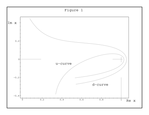
Figure 1: Two samples of the tobogganic curves $x(s)$ obtained as maps of the straight line of $z$ [parameters $\kappa=12/5$ and $\varepsilon=3/20$ and $4/20$ were used in eq. (14)].

Within the space of this letter, an explicit construction of some rectifiable samples of the tobogganic paths can be formulated as our main numerical task. Its solution starts from the choice of the straight-line $z(s)=s-{\rm i}\,\varepsilon$ in the rectified, auxiliary but, presumably, solvable equation (13). We assume that the change of variables (14) is implemented here in such a manner that it returns us strictly back to the input, tobogganic bound-state eigenvalue problem of eq. (12).

The knot-like structure of the curves $x^{\varrho_{0}}(s)$ is most easily visualized when one proceeds from a straight-line $z(s)=s-{\rm i}\,\varepsilon$. Using the standard computer graphics facilities, we can only vary the exponent $\kappa>1$ and employ the mapping ${\cal M}:z(s)\to x(s)$ given by eq. (14). Such an inverse transformation maps the straight lines $z(s)$ backwards into the equivalent, $\varepsilon-$dependent tobogganic contours ${x}^{(\varrho_{0})}(s)$ where the structure of the descriptor word $\varrho_{0}$ is to be inferred from a detailed analysis of the graphs and pictures.

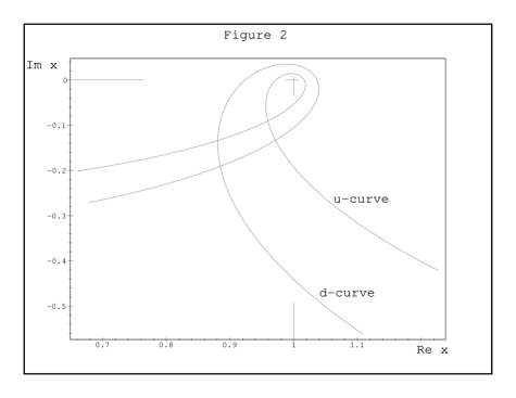
Figure 2: Similar curves as in Figure 1, at the exponent $\kappa=3$.

In the illustrative Figure 1 we choose $\kappa=2.4$ and restricted the parameter $s$ to a finite interval between $s=0.4$ and $s=1.4$. We also selected the two (viz., up- and down-lying) “representative” samples of the parameter $\varepsilon=\varepsilon_{u}=0.15$ and $\varepsilon=\varepsilon_{d}=0.2$. This enabled us to illustrate that and how the explicit shapes and qualitative features of the resulting curves ${x}^{(\varrho_{0})}(s)$ can vary. In order to guide the eye, we also emphasized the location of the branch point $x^{(BP)}=+1$.

When we choose a bigger exponent $\kappa=3$, we accelerate the winding so that our tobogganic spirals $x(s)$ move more quickly downwards and to the right (cf. Figure 2).

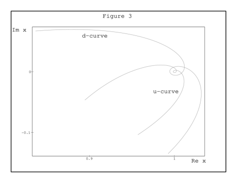
Figure 3: Similar curves as in Figures 1 and 2, at $\kappa=5$.

When we further increase the value of the exponent to $\kappa=5$, both our spirals will turn twice around the singularities $\pm 1$ and, with the further growth of $s$, they will continue moving downwards and to the right in complex plane. In Figure 3 we choose $s\in(0.55,1.285)$ to show, in more detail, how both our spirals “orbit” around the point $x^{(BP)}_{+}=1$.

5.3 Effective non-tobogganic ${\cal PT}-$symmetric potentials

The most important consequence of the preceding graphical exercises is twofold. Firstly we see that they represent the easiest way of the determination of the rectifiable descriptors $\varrho_{0}$. Secondly, the closed and compact formulae are at our disposal. The latter merit of our recipe enables us to differentiate eq. (14), yielding the relation between the two differential operators

$$\frac{d}{d\,x}=\beta(z)\,\frac{d}{d\,z}\,,\ \ \ \ \ \ \beta(z)=-{\rm i}\,\frac{\sqrt{(1-z^{2})^{\kappa}-1}}{\kappa\,z\,(1-z^{2})^{\kappa-1}}\,.$$

Together with the usual ansatz $\psi(x)=\chi(z)\,\varphi(z)$ and with an abbreviation for the effective potential $V_{eff}({\rm i}\,x)=V({\rm i}\,x)+2\,\ell(\ell+1)[1-({\rm i}\,x)^{2}]/[1+({\rm i}\,x)^{2}]^{2}$, the latter formula may be inserted in our fundamental differential Schrödinger eq. (12) yielding

$$\left(-\beta(z)\,\frac{d}{dz}\,\beta(z)\,\frac{d}{dz}+V_{eff}[ix(z)]-E\right)\,\chi(z)\,\varphi(z)=0\,.$$

The choice of $\chi(z)=const\,/\sqrt{\beta(z)}$ (which dates back to Liouville [13]) enables us to eliminate the first derivative of $\varphi(z)$ and to simplify the latter equation to its final Schrödinger form (13). One only has to add the definition

$$U_{eff}({\rm i}\,z)=\frac{V_{eff}[{\rm i}\,x(z)]-E_{n}}{\beta^{2}(z)}+\frac{\beta^{\prime\prime}(z)}{2\,\beta(z)}-\frac{[\beta^{\prime}(z)]^{2}}{4\,\beta^{2}(z)}$$ (15)

where the prime denotes the differentiation with respect to $z$. Our task is completed since the ${\cal PT}-$symmetry of the latter formula is obvious. By the way, it is also amusing to notice that in the limit of the large $x$ and/or $z$, our final formula (15) degenerates to its single-spire predecessor of refs. [8, 9] exemplified also here, in paragraph 3.2, by its sextic-oscillator illustration (10).

6 Conclusions

We saw that the introduction of quantum toboggans may be understood as a mere slight innovation of the traditional quantization recipes [7, 14]. Still, in our present extension of the results of papers [8, 9] we demonstrated that this innovation may still lead to certain very nontrivial consequences, especially in the context of building phenomenological models in Quantum Mechanics or even beyond its scope like, say, in classical magnetohydrodynamics [15] etc.

Our present main result is that for each individual potential $V(x)$ and for each individual choice of the specific, sufficiently simple topology (i.e., descriptor $\varrho=\varrho_{0}$) of the QT2 path $x^{(\varrho_{0})}$, the necessary proof of the reality/observability of the energies becomes trivial, based on the mere change of variables given by closed formulae. Thus, the “measurable predictions” (i.e., the bound-state energies) of our $\varrho=\varrho_{0}$ subset of the QT2 models prove observable if and only if the ${\cal PT}-$symmetry of the equivalent rectified problem (13) remains unbroken [7].

In a broader context with any descriptor $\varrho$ we showed that the ${\cal PT}-$symmetric quantum toboggans with the left-right symmetric doublet of branching points can be enumerated and classified using a certain “word” form of the generalization of the winding number as used in the most elementary model of ref. [8].

We also discussed in some technical detail how one replaces the tobogganic Schrödinger equation (exhibiting a generalized ${\cal PT}-$symmetry as described in [9]) by its equivalent representation with the usual ${\cal PT}-$symmetry defined in the cut complex plane. We paid attention to the fact that the rectified, non-tobogganic version of our QT2 Schrödinger bound-state problem contains a more complicated form of the effective potential, which is the price to be paid for its simplified definition along an elementary straight line in the complex plane of $z(s)$.

Obviously, every successful and, in particular, analytic rectification of ${x^{(QT)}(s)}$ (including, of course, it present concrete samples) always opens immediately a way to the translation of a given tobogganic bound-state problem into its standard straight-line avatar. Thus, in a way which represents a straightforward QT2 extension of the single-spire QT1 recipe of ref. [8], the existence of the present one-parametric and compact rectification formula (14) may be expected to faciliatate an application of the standard numerical as well as purely analytic techniques of the explicit construction of the QT2 bound states at $\varrho=\varrho_{0}$.

Vice versa, the possibility of proceeding in the opposite direction (i.e., from a trivial contour $z^{(0)}$ to its nontrivial QT2 descendant with $\varrho=\varrho_{0}\neq 0$) is of particular appeal in mathematics because in the direction from the straight line to a tobogganic curve, it enables us to generate a number of the exactly solvable models with the real spectra (i.e., of phenomenological interest).

It is pleasing to see the reducibility of the key problem of the proof of the reality of the spectrum to the mere technicality of an appropriate change of variables. The study of its pragmatic computational consequences has been omitted from the present text but it may prove equally important in applications. Indeed, one could find the equivalence between some tobogganic and non-tobogganic models particularly appealing in the context of physics.

In many topologically nontrivial Schrödinger eigenvalue problems, the rectification, whenever feasible, would simplify significantly the explicit and detailed computations of the topology-dependent spectra. As long as these computations might be fairly difficult, several detailed numerical studies of this type (paying attention to the most elementary interaction potentials $V(x)$) are already under preparation at present [16, 17].

Figure captions

Figure 1. Two samples of the tobogganic curves $x(s)$ obtained as maps of the straight line of $y$ [parameters $\kappa=12/5$ and $\varepsilon=3/20$ and $4/20$ were used in eq. (14)].

Figure 2. Similar curves as in Figure 1, at the exponent $\kappa=3$.

Figure 3. Similar curves as in Figures 1 and 2, at $\kappa=5$.

References

- [1] Sibuya Y 1975 Global Theory of Second Order Linear Differential Equation with Polynomial Coefficient (Amsterdam: North Holland); Alvarez G 1995 J. Phys. A: Math. Gen. 27 4589
- [2] Caliceti E, Graffi S and Maioli M 1980 Commun. Math. Phys. 75 51
- [3] Buslaev V and Grechi V 1993 J. Phys. A: Math. Gen. 26 5541
- [4] Bender C M and Turbiner A V 1993 Phys. Lett. A 173 442
- [5] Bender C M and Boettcher S 1998 Phys. Rev. Lett. 80 5243
- [6] Bender C M, Boettcher S and Meisinger P N 1999 J. Math. Phys. 40 2201
- [7] C. M. Bender, Rep. Prog. Phys., submitted (hep-th/0703096).
- [8] Znojil M 2005 Phys. Lett. A 342 36
- [9] Znojil M 2006 J. Phys. A: Math. Gen. 39 13325
- [10] Znojil M 1999 Phys. Lett. A 259 220
- [11] Dorey P, Dunning C and Tateo R 2001 J. Phys. A: Math. Gen. 34 5679 and L391; Shin K C 2002 Commun. Math. Phys. 229 543
- [12] Sinha A and Roy P 2004 Czechosl. J. Phys. 54 129
- [13] Liouville L 1837 J. Math. Pures Appl. 1 16
- [14] Scholtz F G, Geyer H B and Hahne F J W 1992 Ann. Phys. (NY) 213 74
- [15] Znojil M and Günther U 2007 J. Phys. A: Math. Theor. 40 7375.
- [16] Znojil M, Tater M and Günther U, in preparation
- [17] Wessels G et al, in preparation