A multi-objective optimization procedure to develop modified-embedded-atom-method potentials: an application to magnesium

Abstract

We have developed a multi-objective optimization (MOO) procedure to construct modified-embedded-atom-method (MEAM) potentials with minimal manual fitting. This procedure has been applied successfully to develop a new MEAM potential for magnesium. The MOO procedure is designed to optimally reproduce multiple target values that consist of important materials properties obtained from experiments and first-principles calculations based on density-functional theory (DFT). The optimized target quantities include elastic constants, cohesive energies, surface energies, vacancy formation energies, and the forces on atoms in a variety of structures. The accuracy of the new potential is assessed by computing several material properties of Mg and comparing them with those obtained from other potentials previously published. We found that the present MEAM potential yields a significantly better overall agreement with DFT calculations and experiments.

I Introduction

Molecular dynamics simulations are effective tools used to study many interesting phenomena such as the melting and coalescence of nanoparticles at the atomic scale.J.-H. et al. (2002); Kim and Tománek (1994) These atomistic simulations require accurate interaction potentials to compute the total energy of the system, and first-principles calculations can provide the most reliable interatomic potentials. However, realistic molecular dynamics simulations often require an impractical number of atoms that either demands too much computer memory or takes too long to be completed in a reasonable amount of time. One alternative is to use empirical or semi-empirical interaction potentials that can be evaluated efficiently.

The modified-embedded-atom method (MEAM) proposed by Baskes et al.Baskes et al. (1989); Baskes (1992); Baskes and Johnson (1994) is one of the most widely used methods using semi-empirical atomic potentials to date. The MEAM is an extension of the embedded-atom method (EAM) to include angular forces.Daw and Baskes (1983, 1984); Baskes (1987) The MEAM and EAM use a single formalism to generate semi-empirical potentials that have been successfully applied to a large variety of materials including fcc, bcc, hcp, diamond-structured materials and even gaseous elements, to produce simulations in good agreement with experiments or first-principles calculations.Baskes (1987); Baskes et al. (1989); Baskes (1992); Baskes and Johnson (1994)

Despite its remarkable successes, one of the most notable difficulties in using MEAM is that the construction of the MEAM potentials involves a lot of manual and ad hoc fittings. Because of the complex relationship between the sixteen MEAM parameters and the resultant behavior of a MEAM potential, a traditional procedure for constructing a MEAM potential involves a two-step iterative process. First, a single crystal structure, designated as the reference structure, is chosen and the MEAM parameters are fitted to construct a MEAM potential that reproduces a handful of critical materials properties of the element in the reference structure. Second, the new potential is tested for its accuracy and transferrability by applying it to atoms under circumstances not used during its construction phase. These systems include different crystal structures, surfaces, stacking faults, and point defects. If the validation is not satisfactory, one needs to go back to the first step and adjust the parameters in a way that improves the overall quality of the potential. Although this iterative method does work eventually in many cases, it is a very tedious and time-consuming. Ercolessi and Adams overcame this shortcoming for EAM potentials by developing a force-matching method that fits the EAM potential to ab initio atomic forces of many atomic configurations including surfaces, clusters, liquids and crystals at finite temperature.Ercolessi and Adams (1994) Later, the force-matching method was extended to include many other materials properties such as cohesive energy, lattice constants, stacking fault energies, and elastic constants.Liu et al. (1996); Li et al. (2003) Furthermore, several different MEAM potentials for the same element often develop and an objective and quantitative method to measure the relative quality of each potential would be helpful for the researchers who want to choose one of these potentials.

In this work, we extend the force-matching method to develop a multi-objective optimization (MOO) procedure to construct MEAM potentials. Most realistic optimization problems, particularly in engineering, require the simultaneous optimization of more than one objective function. For example, aircraft design requires simultaneous optimization of fuel efficiency, payload and weight calls for a MOO procedure. In most cases, it is unlikely that the different objectives would be optimized by the same parameter choices. Therefore, some trade-off between the objectives is needed to ensure a satisfactory design. StadlerW. (1979) introduced the concept of Pareto optimalityPareto (1909) to the fields of engineering and science. The most widely used method for multi-objective optimization is the weighted sum method. A comprehensive overview and comparison of different MOO methods can be found in Ref. Andersson, 2001.

The composite objective function also provides an unbiased measure to quantify the relative quality of different MEAM potentials. We apply the procedure to develop a new MEAM potential for magnesium. The new Mg MEAM potential will be compared with previously published Mg potentials.

We chose Mg bacause of its increased importantance in many technological areas, including the aerospace and automotive industries. Due to the lower mass densities of magnesium alloys compared with steel and aluminum and higher temperature capabilities and improved crash-worthiness than plastics, the use of magnesium die castings is increasing rapidly in the automotive industry. Han et al. (2005); Lou et al. (1995); Pettersen et al. (1996)

Empirical potentials for Mg have been previously proposed by several groups. In 1988, Oh and Johnson developed analytical EAM potentials for hcp metals such as Mg.Oh and Johnson (1988) Igarashi, Kanta and VitekIgarashi et al. (1991) (IKV) also developed interatomic potentials for eight hcp metals including Mg using the Finnis–Sinclair type many-body potentials.Finnis and Sinclair (1984) Pasianot and SavinoPasianot and Savino (1992) proposed improved EAM potentials for Mg based on IKV’s fitting scheme. Baskes and Johnson Baskes and Johnson (1994) have extended the modified embedded atom method (MEAM) Baskes (1987); Baskes et al. (1989); Baskes (1992) to hcp crystal structures. Later, Jelinek et al. improved this potential as a part of the MEAM potentials for Mg-Al alloy system.Jelinek et al. (2007) Liu et al. used the force-matching method to develop an EAM potential for Mg.Liu et al. (1996)

The paper is organized in the following manner. In Sec. II, we give a brief review of the MEAM. In Sec. III, the procedure for determination of the MEAM parameters is presented in detail. In Sec. IV, we assess the accuracy and transferability of our MEAM potential and make comparisons to other previously published potentials.

II Methodology

II.1 MEAM

The total energy $E$ of a system of atoms in the MEAM Kim et al. (2006) is approximated as the sum of the atomic energies

$$E=\sum_{i}E_{i}.$$ (1)

The energy of atom $i$ consists of the embedding energy and the pair potential terms:

$$E_{i}=F_{i}(\bar{\rho}_{i})+\frac{1}{2}\sum_{j\neq i}\phi_{ij}(r_{ij}).$$ (2)

$F_{i}$ is the embedding function of atom $i$; $\bar{\rho}_{i}$ is the background electron density at the site of atom $i$; and $\phi_{ij}(r_{ij})$ is the pair potential between atoms $i$ and $j$ separated by a distance $r_{ij}$. The embedding energy $F_{i}(\bar{\rho}_{i})$ represents the energy cost to insert atom $i$ at a site where the background electron density is $\bar{\rho}_{i}$. The embedding energy is given in the form

$$F_{i}(\bar{\rho}_{i})=A_{i}E_{i}^{0}\bar{\rho}_{i}\ln(\bar{\rho}_{i}),$$ (3)

where the parameters $E_{i}^{0}$ and $A_{i}$ depend on the element type of atom $i$. The background electron density $\bar{\rho}_{i}$ is given by

$$\bar{\rho}_{i}=\frac{\rho_{i}^{(0)}}{\rho_{i}^{0}}G(\Gamma_{i}),$$ (4)

where

$$\Gamma_{i}=\sum_{k=1}^{3}\bar{t}_{i}^{(k)}\left(\frac{\rho_{i}^{(k)}}{\rho_{i}^{(0)}}\right)^{2}$$ (5)

and

$$G(\Gamma)=\sqrt{1+\Gamma}.$$ (6)

The zeroth and higher order densities, $\rho_{i}^{(0)}$, $\rho_{i}^{(1)}$, $\rho_{i}^{(2)}$, and $\rho_{i}^{(3)}$ are given in Eq. (9). The composition-dependent electron density scaling $\rho_{i}^{0}$ is given by

$$\rho_{i}^{0}=\rho_{i0}Z_{i0}G(\Gamma_{i}^{\text{ref}}),$$ (7)

where $\rho_{i0}$ is an element-dependent density scaling, $Z_{i0}$ is the first nearest-neighbor coordination of the reference system, and $\Gamma_{i}^{\text{ref}}$ is given by

$$\Gamma_{i}^{\text{ref}}=\frac{1}{Z_{i0}^{2}}\sum_{k=1}^{3}\bar{t}_{i}^{(k)}s_{i}^{(k)},$$ (8)

where $s_{i}^{(k)}$ is the shape factor that depends on the reference structure for atom $i$. Shape factors for various structures are specified in the work of BaskesBaskes (1992). The partial electron densities are given by

$$\rho_{i}^{(0)} = \sum_{j\neq i}\rho_{j}^{a(0)}S_{ij}$$ (9a)

$$\left(\rho_{i}^{(1)}\right)^{2} = \sum_{\alpha}\left[\sum_{j\neq i}\rho_{j}^{a(1)}\frac{r_{ij\alpha}}{r_{ij}}S_{ij}\right]^{2}$$ (9b)

$$\left(\rho_{i}^{(2)}\right)^{2} = \sum_{\alpha,\beta}\left[\sum_{j\neq i}\rho_{j}^{a(2)}\frac{r_{ij\alpha}r_{ij\beta}}{r_{ij}^{2}}S_{ij}\right]^{2}$$ (9c)

$$-\frac{1}{3}\left[\sum_{j\neq i}\rho_{j}^{a(2)}S_{ij}\right]^{2}$$

$$\left(\rho_{i}^{(3)}\right)^{2} = \sum_{\alpha,\beta,\gamma}\left[\sum_{j\neq i}\rho_{j}^{a(3)}\frac{r_{ij\alpha}r_{ij\beta}r_{ij\gamma}}{r_{ij}^{3}}S_{ij}\right]^{2}$$ (9d)

$$-\frac{3}{5}\sum_{\alpha}\left[\sum_{j\neq i}\rho_{j}^{a(3)}\frac{r_{ij\alpha}}{r_{ij}}S_{ij}\right]^{2},$$

where $r_{ij\alpha}$ is the $\alpha$ component of the displacement vector from atom $i$ to atom $j$. $S_{ij}$ is the screening function between atoms $i$ and $j$ and is defined in Eqs. (16). The atomic electron densities are computed as

$$\rho_{i}^{a(k)}(r_{ij})=\rho_{i0}\exp\left[-\beta_{i}^{(k)}\left(\frac{r_{ij}}{r_{i}^{0}}-1\right)\right],$$ (10)

where $r_{i}^{0}$ is the nearest-neighbor distance in the single-element reference structure and $\beta_{i}^{(k)}$ are element-dependent parameters. Finally, the average weighting factors are given by

$$\bar{t}_{i}^{(k)}=\frac{1}{\rho_{i}^{(0)}}\sum_{j\neq i}t_{j}^{(k)}\rho_{j}^{a(0)}S_{ij},$$ (11)

where $t_{j}^{(k)}$ is an element-dependent parameter.

The pair potential is given by

$$\phi_{ij}(r_{ij}) =\bar{\phi}_{ij}(r_{ij})S_{ij}$$ (12)

$$\begin{split}\bar{\phi}_{ij}(r_{ij})&=\frac{1}{Z_{ij}}\left[2E_{ij}^{u}(r_{ij})-F_{i}\left(\frac{Z_{ij}\rho^{(0)}_{j}(r_{ij})}{Z_{i}\rho^{0}_{i}}\right)\right.\\ &\quad\left.-F_{j}\left(\frac{Z_{ij}\rho^{(0)}_{i}(r_{ij})}{Z_{j}\rho^{0}_{j}}\right)\right]\end{split}$$ (13)

$$E_{ij}^{u}(r_{ij}) =-E^{0}_{ij}\left(1+a_{ij}^{*}(r_{ij})\right)e^{-a_{ij}^{*}(r_{ij})}$$ (14)

$$a_{ij}^{*} =\alpha_{ij}\left(\frac{r_{ij}}{r_{ij}^{0}}-1\right),$$ (15)

where $\alpha_{ij}$ is an element-dependent parameter. The sublimation energy $E^{0}_{ij}$, the equilibrium nearest-neighbor distance $r_{ij}^{0}$, and the number of nearest-neighbors $Z_{ij}$ are obtained from the reference structure.

The screening function $S_{ij}$ is designed so that $S_{ij}=1$ if atoms $i$ and $j$ are unscreened and within the cutoff radius $r_{c}$, $S_{ij}=0$ if they are completely screened or outside the cutoff radius, and varies smoothly between 0 and 1 for partial screening. The total screening function is the product of a radial cutoff function and three-body terms involving all other atoms in the system:

$$S_{ij} =\bar{S}_{ij}f_{c}\left(\frac{r_{c}-r_{ij}}{\Delta r}\right)$$ (16a)

$$\bar{S}_{ij} =\prod_{k\neq i,j}S_{ikj}$$ (16b)

$$S_{ikj} =f_{c}\left(\frac{C_{ikj}-C_{\text{min},ikj}}{C_{\text{max},ikj}-C_{\text{min},ikj}}\right)$$ (16c)

$$C_{ikj} =1+2\frac{r_{ij}^{2}r_{ik}^{2}+r_{ij}^{2}r_{jk}^{2}-r_{ij}^{4}}{r_{ij}^{4}-\left(r_{ik}^{2}-r_{jk}^{2}\right)^{2}}$$ (16d)

$$f_{c}\left(x\right) =\begin{cases}1&x\geq 1\\ \left[1-\left(1-x)^{4}\right)\right]^{2}&0<x<1\\ 0&x\leq 0\\ \end{cases}$$ (16e)

Note that $C_{\text{min}}$ and $C_{\text{max}}$ can be defined separately for each $i$-$j$-$k$ triplet, based on their element types. The parameter $\Delta r$ controls the distance over which the radial cutoff function changes from 1 to 0 near $r=r_{c}$.

II.2 Multi-objective Optimization

A generic multi-objective optimization (MOO) problem can be formulated as Kim and de Weck (2005); deW (2004):

$$\begin{split}\min\ &\mathbf{J}(\mathbf{x})\quad\text{s.t.}\quad x\in S\\ \text{where}\ \mathbf{J}&=[J_{1}(\mathbf{x})\cdots J_{m}(\mathbf{x})]^{T}\\ \mathbf{x}&=[x_{1}\cdots x_{n}]^{T}\\ \end{split}$$ (17)

Here, $\mathbf{J}$ is a column vector of $m$ objectives, whereby $J_{i}\in\mathds{R}$. The individual objectives are dependent on a vector $\mathbf{x}$ of $n$ design variables in the feasible domain $S$. The design variables are assumed to be continuous and vary independently. Typically, the feasible design domain is defined by the design constraints and the bounds on the design variables. The problem is to minimize all elements of the objective vector simultaneously. The most widely used method for MOO is scalarization using the weighted sum method. The method transforms the multiple objectives into an aggregated scalar objective function $J$ that is the sum of each objective function $J_{i}$ multiplied by a positive weighting factor $w_{i}$:

$$J(\mathbf{x})=\sum_{i=1}^{m}w_{i}J_{i}(\mathbf{x}).$$ (18)

In this work, the overall goal is to develop a MEAM potential for Mg. The individual objective functions are constructed from the normalized differences between the MEAM-generated values and the target values:

$$J_{i}(\mathbf{x})=\left[\frac{Q_{i}(\mathbf{x})-Q_{i}^{0}}{Q_{i}^{*}}\right]^{2}.$$ (19)

Here, $Q_{i}$ is the physical quantity computed using the current MEAM potential parameters and $Q_{i}^{0}$ is the target value to reproduce. The target values are usually experimental values, but the computed values from the first-principles method are chosen when the experimental data are not available. The normalization factor $Q_{i}^{*}$ is a typical value for the given materials parameter and often $Q_{i}^{*}=Q_{i}^{0}$. The overall objective function $J(\mathbf{x})$ can be minimized using usual multi-dimensional otimization routines. To avoid unnecessary complications, we used the downhill simplex method,Press et al. (1992) which requires only function evaluations, not derivatives.

III Potential Construction Procedure

We used the MOO procedure to develop a new set of MEAM parameters that improves the overall agreement of MEAM results with experiments or ab initio calculations. Our previously published MEAM parameters for MgJelinek et al. (2007) served as the basis for the present work.

All ab initio total-energy calculations and geometry optimizations are performed within density functional theory (DFT) using ultrasoft pseudopotentials (USPP) Vanderbilt (1990) as implemented by Kresse et. al.Kresse and Hafner (1994); Kresse and Furthmüller (1996) For the treatment of electron exchange and correlation, we use local-density approximation (LDA)D. M. Ceperley and B. J. Alder (1980); J. P. Perdew and A. Zunger (1981). The Kohn-Sham equations are solved using a preconditioned band-by-band conjugate-gradient (CG) minimization.Kresse and Hafner (1993) The plane-wave cutoff energy is set to at least 300 eV in all calculations. Geometry relaxations are performed until the energy difference between two successive ionic optimizations is less than 0.001 eV. The Brillouin zone is sampled using the Monkhorst-Pack schemeMonkhorst and Pack (1976) and a Fermi-level smearing of 0.2 eV was applied using the Methfessel-Paxton method.Methfessel and Paxton (1989)

The objectives used in this work include equilibrium hcp lattice constants $a$ and $c$ at 0 K, the cohesive energy, elastic constants, vacancy formation energy, surface energies, stacking fault energies, and adsorption energies. We also used the forces on Mg atoms in structures equilibriated at six different temperatures. The final MEAM parameters obtained from the MOO procedure are listed in Table 1. Table 2 shows the complete list of objectives optimized to construct the MEAM potential parameters for Mg and their weights.

III.0.1 Cohesive energies

The cohesive energy of Mg atom is defined as the heat of formation per atom when Mg atoms are assembled into a crystal structure:

$$E_{\text{coh}}=\frac{E_{\text{tot}}-NE_{\text{atom}}}{N},$$ (20)

where $E_{\text{tot}}$ is the total energy of the system, $N$ is the number of Mg atoms in the system, and $E_{\text{atom}}$ is the total energy of an isolated Mg atom. The cohesive energies of Mg atoms in hcp, fcc, and bcc crystal structures for several atomic volumes near the equilibrium atomic volumes were calculated. Fig. 1 is an example of the cohesive energy plot of Mg atoms as a function of the lattice constant. The minimum of this curve determines the equilibrium lattice constant $a_{0}$ and equilibrium cohesive energies $E_{\text{hcp}}=E_{\text{hcp}}$ in Table 2.

III.0.2 Elastic constants

Hexagonal crystals have five independent elastic constants: $C_{11}$, $C_{12}$, $C_{13}$, $C_{33}$, and $C_{44}$.Ledbetter (1977) The elastic constants are calculated numerically by applying small strains to the lattice. For small deformations, the relationship between deformation strain and elastic energy increase in an hcp crystal is quadratic:Liu et al. (1996)

1. $\Delta U=\delta^{2}(C_{11}+C_{12})$, for deformation $x^{\prime}=x+\delta\cdot x$, $y^{\prime}=y+\delta\cdot y$,

2. $\Delta U=\delta^{2}(C_{11}-C_{12})$, for deformation $x^{\prime}=x+\delta\cdot x$, $y^{\prime}=y-\delta\cdot y$,

3. $\Delta U=\delta^{2}C_{33}/2$, for deformation $z^{\prime}=z+\delta\cdot z$,

4. $\Delta U=\delta^{2}(2C_{11}+C_{33}+2C_{12}+4C_{13})/2$, for deformation $x^{\prime}=x+\delta\cdot x$, $y^{\prime}=y+\delta\cdot y$, $z^{\prime}=z+\delta\cdot z$,

5. $\Delta U=\delta^{2}C_{44}/2$, for deformation $z^{\prime}=z+\delta\cdot x$,

where unprimed (primed) are the coordinates of the lattice before (after) deformation. $\Delta U$ is the elastic energy due to the deformation, and $\delta$ is the small strain applied to the lattice. We follow the procedure described by Mehl et al.Mehl et al. (1994) and apply several different strains ranging from $-2.0$% to $+2.0$%. The elastic constants are obtained by fitting the resultant curves to quadratic functions. We found that this method gives much more stable results than using one strain valueLiu et al. (1996).

III.0.3 Surface formation energies

Surface formation energy per unit surface area is defined as

$$\gamma=\left(E_{\text{tot}}-N\varepsilon\right)/A,$$ (21)

where $E_{\text{tot}}$ is the total energy of the system with a surface, $N$ is the number of atoms in the system, $\varepsilon$ is the total energy per atom in the bulk, and $A$ is the surface area. Table 2 lists the surface formation energies used in this study. The (10$\bar{1}$0) surface of hcp crystals can be terminated in two ways, either with a short first interlayer distance $d_{12}$ (“short termination”) or with a long $d_{12}$ (“long termination”) (See, for example, Fig. 2 of Ref. Hofmann et al., 1996). In this study, we only included the results for the short terminated surface, since it is known to be enegetically more favorable over the long terminated surface Staikov and Rahman (1999) in agreement with experimental observations in Be(10$\bar{1}$0) and other hcp metals.Hofmann et al. (1996)

III.0.4 Stacking fault energies

Stacking fault formation energy per unit area is defined by

$$E_{\text{sf}}=\left(E_{\text{tot}}-N\varepsilon\right)/A,$$ (22)

where $E_{\text{tot}}$ is the total energy of the structure with a stacking fault, $N$ is the number of atoms in the system, $\varepsilon$ is the total energy per atom in the bulk, and $A$ is the unit cell area that is perpendicular to the stacking fault. For Mg, four stacking fault types from the calculation of Chetty et al.Chetty and Weinert (1997) were examined. The sequences of the atomic layers within the unit cell of our simulations are: $I_{1}=ABABABCBCBCB$, $I_{2}=ABABABCACACB$, $T_{2}=ABABABCBABAB$, and $E=ABABABCABABAB$. We note that the unit cells for $I_{1}$ and $I_{2}$ contain two stacking faults and the quantities obtained from Eq. (22) must be divided by two to obtain the correct formation energies.

III.0.5 Vacancy formation energies

The formation energy of a single vacancy $E_{\text{vac}}$ is defined as the energy cost to create a vacancy:

$$E_{\text{vac}}=E_{\text{tot}}[N]-N\varepsilon,$$ (23)

where $E_{\text{tot}}[N]$ is the total energy of a system with $N$ atoms containing a vacancy, and $\varepsilon$ is the energy per atom in the bulk.

III.0.6 Atomic Forces

For forces, the objective functions are defined as:

$$J_{i}(\mathbf{x})=\frac{(\left<(\mathbf{F}-\mathbf{F}^{0})^{2}\right>)^{1/2}}{(\left<(\mathbf{F}^{0})^{2}\right>)^{1/2}},$$ (24)

where $\mathbf{F}$ are the force vectors on atoms calculated using the MEAM while $\mathbf{F}^{0}$ are the force vectors from DFT method. $(\left<(\mathbf{F}^{0})^{2}\right>)^{1/2}$ represents the root-mean-square of the DFT force, and $(\left<(\mathbf{F}-\mathbf{F}^{0})^{2}\right>)^{1/2}$ is the root-mean-square of the error in the force.

To obtain the force data, initial atomic structures that contain 180 Mg atoms were created from the bulk hcp crystal structure. The positions of atoms are randomly disturbed from their equilibrium positions and $10\,000$ steps of molecular-dynamics (MD) simulations with a timestep of $\Delta t$ = 2.5 ps were performed to equilibrate each structure for different temperatures. In each MD run, we used Mg MEAM potential by Jelinek et al.Jelinek et al. (2007) If no MEAM potential were available for MD simulations, one could use an intermediate MEAM potential that is generated with this MOO procedure without the force data. The potential should be adequate enough to obtain a reasonable set of structures.

IV Results and Discussion

The hcp structure was chosen as the reference structure for Mg. The final MEAM parameters obtained from the MOO procedure are listed in Table 1.

Table 1: Set of the MEAM potential parameters for Mg. See Sec. II.1 for the definition of these parameters and their usage. The hcp structure was chosen as the reference structure for Mg.

$E^{0}$[eV]	$a_{0}$[Å]	$A$	$\alpha$	$\beta^{(0)}$	$\beta^{(1)}$	$\beta^{(2)}$	$\beta^{(3)}$	$t^{(0)}$	$t^{(1)}$	$t^{(2)}$	$t^{(3)}$	$C_{\text{max}}$	$C_{\text{min}}$	$r_{c}$	$\Delta r$
1.51	3.20	1.14	5.69	2.66	-0.003	0.348	3.32	1.00	8.07	4.16	-2.02	3.22	1.10	5.0	0.353

IV.1 Materials properties

Table 2: The objectives optimized to construct the MEAM potential parameters for Mg along with the target values and their weights. Comparisons to other Mg potentials are also made. $E_{\text{coh}}$ is the cohesive energy, $B$ is the bulk modulus, $\gamma$ is the surface energy, $E_{\text{sf}}$ is the stacking fault formation energy, $E_{\text{vac}}$ is the relaxed vacancy formation energy, and $\Delta\mathbf{F}$ is the relative error in forces. The underlined quantities are the target values chosen for the MOO procedure.

	Objective	Unit	Weight	Expt	DFT	MEAM	Jelinek	Liu	Hu
1	$a_{0}$	Å	1.0	3.21 [Emsley, 1998]	3.128	3.21	3.21	3.21
2	$c/a$	-	1.0	1.623 [Emsley, 1998]	1.623	1.622	1.623	1.623
3	$E_{\text{coh}}=E_{\text{hcp}}$	eV	2.0	1.51 [Kittel, 1996]	1.78	1.51	1.55	1.52
4	$B$	kbar	1.0	369 [Smith, 1976]		376	353	367
5	$E_{\text{fcc}}-E_{\text{hcp}}$	meV	0.72		14 [Althoff et al., 1993]	4	4	15
6	$E_{\text{bcc}}-E_{\text{hcp}}$	meV	0.72		29 [Althoff et al., 1993]	34	30	18
7	$C_{11}$	kbar	1.0	635 [Smith, 1976]		606	602	618
8	$C_{12}$	kbar	1.0	260 [Smith, 1976]		274	237	259
9	$C_{13}$	kbar	1.0	217 [Smith, 1976]		250	219	219
10	$C_{33}$	kbar	1.0	665 [Smith, 1976]		631	623	675
11	$C_{44}$	kbar	1.0	184 [Smith, 1976]		151	155	182
12	$\gamma[(0001)]$	mJ/m2	1.0	680 [Tyson and Miller, 1977]	637	583	595	495	310
13	$\gamma[(10\bar{1}0)]$	mJ/m2	1.0		721	625	645
14	$E_{\text{sf}}[I_{1}]$	eV	0.1		18	8	7	27	4
15	$E_{\text{sf}}[I_{2}]$	eV	0.1		37	15	15	54	8
16	$E_{\text{sf}}[T_{2}]$	eV	0.1		45	15	15
17	$E_{\text{sf}}[E]$	eV	0.1		61	23	22		12
28	$E_{\text{vac}}$	eV	1.0	0.58 $\sim$ 0.89	0.82	0.58	0.56	0.87	0.59
19	$\Delta\mathbf{F}$ (100 K)	%	1.0		0.0	38.13	201.51
20	$\Delta\mathbf{F}$ (300 K)	%	1.0		0.0	29.67	93.73
21	$\Delta\mathbf{F}$ (500 K)	%	1.0		0.0	25.18	59.17
22	$\Delta\mathbf{F}$ (800 K)	%	1.0		0.0	25.08	98.77
23	$\Delta\mathbf{F}$ (1000 K)	%	1.0		0.0	26.93	85.31
24	$\Delta\mathbf{F}$ (1200 K)	%	1.0		0.0	27.30	79.77

Table 2 lists various materials properties of Mg selected as the objectives to be optimized in constructing Mg MEAM potential, along with experimental data and ab initio data. It also shows how well each objective has been optimized. Results from other previously published Mg potentials are also listed in the table for comparison. Table 2 also shows the weight of individual objectives $w_{i}$ chosen to optimize the present potential. The underlined quantities are the target values chosen for the MOO procedure. Whenever possible, the experimental values are chosen as the target values. If the experimental values are not available or known to be unreliable, the computed values from the first-principles method are used.

The present MEAM potential reproduces the experimental lattice constant, the $c/a$ ratio, and the cohesive energy near perfectly. Fig. 1 shows the cohesive energies of Mg atoms in hcp crystal structure compared with those obtained from the Rose universal equation of stateRose et al. (1984) based on the experimental lattice constant, cohesive energy and bulk modulus. It shows a good agreement between the two sets of data. We also note that the sequence of the structures is predicted correctly in the order of stability by the present Mg MEAM potential as shown in Table 2.

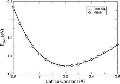
Figure 1: The cohesive energies as a function of the lattice constant $a$ for Mg atoms in hcp crystal structure compared with the ones obtained from the Rose equation. The data points are computed with the present MEAM potential while the curve is obtained from the Rose equation.

The surface formation energies of the two common low-index surfaces of hcp Mg crystals are in good agreement with the experimental values, representing a significant improvement over the previously published MEAM potentials.Jelinek et al. (2007); Lee et al. (2003); Hu et al. (2003)

As pointed out by Liu et al.Liu et al. (1996), the stacking fault energies are difficult quantities for an emprirical potential to reproduce because they only depend on long range interactions beyond second nearest-neighbor distances in hcp crystals. The present MEAM potential shows a substantial improvement over the previously published MEAM potential by Hu et al.Hu et al. (2001) The stacking fault energies are consistently underestimated by the present MEAM potential compared to the results of the DFT calculations, while the results by the EAM potential from Ref. Liu et al., 1996 are consistently overestimated. Table 2 also shows that the formation energy of single vacancies from DFT calculation is reproduced quite reasonably by the present MEAM potential.

Table 2 also shows the force-matching against the ab initio forces database. It shows that the MEAM potential from the present work reproduces more accurate forces on atoms compared to the previous MEAM potentialJelinek et al. (2007).

IV.2 Additional materials properties

Table 3: The additional materials properties of Mg that are not used as objectives for the constructuction of the potential. Comparisons are made to other Mg potentials and experiments. $E_{\text{ads}}$ is the adsorption energy; $E_{\text{f}}^{\text{int}}$ is the formation energies of interstitial point defects. All energy values are given in eV.

Property	DFT	MEAM	Jelinek
$E_{\text{ads}}[(0001)]$	-0.81	-1.46	-1.50
$E_{\text{ads}}[(10\bar{1}0)]$	-1.21	-1.52	-1.56
$E_{\text{f}}^{\text{int}}$ (octahedral)	2.36	1.20	1.29
$E_{\text{f}}^{\text{int}}$ (tetrahedral)	2.35	1.41	1.53

To validate the present MEAM potential further, we calculated a few additional materials properties of Mg that were not used as objectives during the construction of the potential. We obtained the adsorption energies of a single Mg atom on different surfaces and the formation energies of interstitial defects as listed in Table 3.

The adsorption energy of a single adatom $E_{\text{ads}}$ is given by

$$E_{\text{ads}}=E_{\text{tot}}-E_{\text{surf}}-E_{\text{atom}},$$ (25)

where $E_{\text{tot}}$ is the total energy of the structure with the adatom adsorbed on the surface, $E_{\text{surf}}$ is the total energy of the surface without the adatom, and $E_{\text{atom}}$ is the total energy of an isolated atom. On both $(0001)$ and $(10\bar{1}0)$ surfaces, we placed a single Mg atom at the site where the atoms of the next layer would normally sit. The structures were then relaxed to determine the adsorption energies. Table 3 shows that the adsorption energies on two Mg surfaces are quite well reproduced by the present MEAM potential. The present Mg potential gives slightly better adsorption energies than the previously published MEAM potential Jelinek et al. (2007).

The formation energy of an interstitial point defect $E_{\text{f}}^{\text{int}}$ is given by

$$E_{\text{f}}^{\text{int}}=E_{\text{tot}}[N+1]-(E_{\text{tot}}[N]+\varepsilon),$$ (26)

where $E_{\text{tot}}[N]$ is the total energy of a system with $N$ Mg atoms, $E_{\text{tot}}[N+1]$ is the total energy of a system with $N$ atoms plus one Mg atom inserted at one of the interstitial sites, and $\varepsilon$ is the total energy per Mg atom in its most stable bulk structure. Interstitial atom formation energies were calculated for Mg at octahedral and tetrahedral sites. Atomic position and volume relaxation were performed. The results of these calculations are listed in Table 3, to be compared with the results from the DFT calculations. The present MEAM potential predicts correct signs for these energies although the magnitudes are about half of those predicted by DFT. MEAM potentials predict that the octahedral site will be more stable than the tetrahedral site, while the DFT calculations indicate that both sites will have nearly the same formation energies.

IV.3 Thermal properties

To validate the new potential for molecular dynamics simulations, we calculated the melting temperatures of pure Mg crystals. We followed a single-phase method as described by Kim and Tománek,Kim and Tománek (1994) in which the temperature is increased at a constant rate and the internal energy of the system is monitored. Fig. 2 shows the internal energies of Mg crystal in hcp structure as a function of temperature. The plot was obtained from the ensemble average of five hcp structures containing 448 Mg atoms. The initial velocity vectors were set randomly according to the Maxwell-Boltzmann velocity distribution at $T=100$ K. The temperature of the system was controlled by using a Nosé-Hoover thermostat.Nosé (1984); Hoover (1985) It is clearly seen from Fig. 2 that the internal energy curve makes an abrupt transition from one linear region to another, marking the melting point. Using this method, we obtained 920 K as the melting temperature of Mg crystals. This result is in good agreement with the experimental value of 923 K. Our result represents a substantial improvement in accuracy from 745 K obtained from a previously published EAM potential Liu et al. (1996) or 780 K from a MEAM potential.Jelinek et al. (2007)

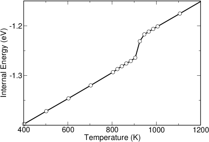
Figure 2: The internal energies of Mg crystal in hcp structure as a function of temperature. The energies are obtained from the ensemble average of the MD simulations of five structures containing 448 Mg atoms.

V Conclusions

In this study, we developed a multi-objective optimization procedure to construct MEAM potentials with minimal manual fitting. We successfully applied this procedure to develop a set of MEAM parameters for Mg interatomic potential based on first-principles calculations within DFT. The validity and transferability of the new MEAM potentials were tested rigorously by calculating the physical properties of the Mg systems in many different atomic arrangements such as bulk, surface, point defect structures, and molecular dynamics simulations. The new MEAM potential shows a significant improvement over previously published potentials, especially for the atomic forces and melting temperature calculations.

VI Acknowledgment

This work has been supported in part by the US Department of Energy under Grant No. DE-AC05-00OR22725 subcontract No. 4000054701. Computer time allocation has been provided by the High Performance Computing Collaboratory (HPC²) at Mississippi State University.

References

- J.-H. et al. (2002) S. J.-H., L. B.-J., and C. Y.W., Surf. Sci. 512, 262 (2002).
- Kim and Tománek (1994) S. G. Kim and D. Tománek, Phys. Rev. Lett. 72, 2418 (1994).
- Baskes et al. (1989) M. I. Baskes, J. S. Nelson, and A. F. Wright, Phys. Rev. B 40, 6085 (1989).
- Baskes (1992) M. I. Baskes, Phys. Rev. B 46, 2727 (1992).
- Baskes and Johnson (1994) M. I. Baskes and R. A. Johnson, Modell. Simul. Mater. Sci. Eng. 2, 147 (1994).
- Daw and Baskes (1983) M. S. Daw and M. I. Baskes, Phys. Rev. Lett. 50, 1285 (1983).
- Daw and Baskes (1984) M. S. Daw and M. I. Baskes, Phys. Rev. B 29, 6443 (1984).
- Baskes (1987) M. I. Baskes, Phys. Rev. Lett. 59, 2666 (1987).
- Ercolessi and Adams (1994) F. Ercolessi and J. Adams, Europhys. Lett. 26, 583 (1994).
- Liu et al. (1996) X.-Y. Liu et al., Modell. Simul. Mater. Sci. Eng. 4, 004 (1996).
- Li et al. (2003) Y. Li et al., Phys. Rev. B 67, 125101 (2003).
- W. (1979) S. W., J. of Optimization Theory and Applications 29, 1 (1979).
- Pareto (1909) V. Pareto, Manuale di Economia Politica (Societa Editrice Libraria, 1909), translated into English by A.S. Schwier as Manual of Political Economy, Macmillan, New York, 1971.
- Andersson (2001) J. Andersson, Ph.D. thesis, Linköping University, Linköping, Sweden (2001).
- Han et al. (2005) Q. Han, K. B. K., and V. Srinath, Philos. Mag. 84, 3843 (2005).
- Lou et al. (1995) A. Lou, J. Renaud, I. Nakatsugawa, and J. Plourde, JOM 47, 28 (1995).
- Pettersen et al. (1996) G. Pettersen, H. Westergen, R. Hoier, and L. O., Mater. Sci. Eng. A 207, 115 (1996).
- Oh and Johnson (1988) D. J. Oh and R. A. Johnson, J. Mater. Res. 3, 471 (1988).
- Igarashi et al. (1991) M. Igarashi, M. Khantha, and V. Vitek, Philos. Mag. B 63, 603 (1991).
- Finnis and Sinclair (1984) M. Finnis and J. Sinclair, Philos. Mag. A 50, 45 (1984).
- Pasianot and Savino (1992) R. Pasianot and E. J. Savino, Phys. Rev. B 45, 12704 (1992).
- Jelinek et al. (2007) B. Jelinek et al., Phys. Rev. B 75, 054106 (pages 9) (2007).
- Kim et al. (2006) Y.-M. Kim, B.-J. Lee, and M. I. Baskes, Phys. Rev. B 74, 014101 (pages 12) (2006).
- Kim and de Weck (2005) I. Y. Kim and O. L. de Weck, Structural and Multidisciplinary Optimization 31, 105 (2005).
- deW (2004) Multiobjective Optimization: History and Promise (The Third China-Japan-Korea Joint Symposium on Optimization of Structural and Mechanical Systems, Kanazawa, Japan, 2004).
- Press et al. (1992) W. H. Press, B. P. Flannery, S. A. Teukolsky, and W. T. Vetterling, Numerical Recipes in C: The Art of Scientific Computing (Cambridge University Press, Cambridge, 1992), 2nd ed.
- Vanderbilt (1990) D. Vanderbilt, Phys. Rev. B 41, 7892 (1990).
- Kresse and Hafner (1994) G. Kresse and J. Hafner, J. Phys.: Cond. Matt. 6, 8245 (1994).
- Kresse and Furthmüller (1996) G. Kresse and J. Furthmüller, Phys. Rev. B 54, 11169 (1996).
- D. M. Ceperley and B. J. Alder (1980) D. M. Ceperley and B. J. Alder, Phys. Rev. Lett. 45, 566 (1980).
- J. P. Perdew and A. Zunger (1981) J. P. Perdew and A. Zunger, Phys. Rev. B 23, 5048 (1981).
- Kresse and Hafner (1993) G. Kresse and J. Hafner, Phys. Rev. B 47, 558 (1993).
- Monkhorst and Pack (1976) H. J. Monkhorst and J. D. Pack, Phys. Rev. B 13, 5188 (1976).
- Methfessel and Paxton (1989) M. Methfessel and A. T. Paxton, Phys. Rev. B 40, 3616 (1989).
- Ledbetter (1977) H. M. Ledbetter, Journal of Physical and Chemical Reference Data 6, 1181 (1977).
- Mehl et al. (1994) M. J. Mehl, B. M. Klein, and D. A. Papaconstantopoulos, in Intermetallic Compounds: Principles and Applications, edited by J. H. Westbrook and R. L. Fleischer (John Wiley & Sons Ltd., London, 1994).
- Hofmann et al. (1996) P. Hofmann, K. Pohl, R. Stumpf, and E. W. Plummer, Phys. Rev. B 53, 13715 (1996).
- Staikov and Rahman (1999) P. Staikov and T. S. Rahman, Phys. Rev. B 60, 15613 (1999).
- Chetty and Weinert (1997) N. Chetty and M. Weinert, Phys. Rev. B 56, 10844 (1997).
- Emsley (1998) J. Emsley, The Elements (Oxford University Press, Oxford, UK, 1998), 3rd ed.
- Kittel (1996) C. Kittel, Introduction to Solid State Physics (John Wiley & Sons, Inc., Hoboken, NJ, 1996), 7th ed.
- Smith (1976) C. J. Smith, ed., Metal Reference Book (Butterworth, Lodon, UK, 1976), 5th ed.
- Althoff et al. (1993) J. D. Althoff et al., Phys. Rev. B 48, 13253 (1993).
- Tyson and Miller (1977) W. R. Tyson and W. A. Miller, Surf. Sci. 62, 267 (1977).
- Hu et al. (2001) W. Hu, B. Zhang, B. Huang, F. Gao, and D. J. Bacon, J. Phys.: Condens. Matter 13, 1193 (2001).
- Rose et al. (1984) J. H. Rose, J. R. Smith, F. Guinea, and J. Ferrante, Phys. Rev. B 29, 2963 (1984).
- Lee et al. (2003) B.-J. Lee, J.-H. Shim, and M. I. Baskes, Phys. Rev. B 68, 144112 (2003).
- Hu et al. (2003) W. Hu, H. Deng, X. Yuan, and M. Fukumoto, Eur. Phys. J. B 34, 429 (2003).
- Nosé (1984) S. Nosé, J. Chem. Phys. 81, 511 (1984).
- Hoover (1985) W. G. Hoover, Phys. Rev. A 31, 1695 (1985).