Evidence for a dynamic phase transition in [Co/Pt]₃ magnetic multilayers

Abstract

A dynamic phase transition (DPT) with respect to the period $P$ of an applied alternating magnetic field has been observed previously in numerical simulations of magnetic systems. However, experimental evidence for this DPT has thus far been limited to qualitative observations of hysteresis loop collapse in studies of hysteresis loop area scaling. Here, we present significantly stronger evidence for the experimental observation of this DPT, in a [Co(4 Å)/Pt(7 Å)]₃-multilayer system with strong perpendicular anisotropy. We applied an out-of-plane, time-varying (sawtooth) field to the [Co/Pt]₃ multilayer, in the presence of a small additional constant field, $H_{b}$. We then measured the resulting out-of-plane magnetization time series to produce nonequilibrium phase diagrams (NEPDs) of the cycle-averaged magnetization, $Q$, and its variance, $\sigma^{2}(Q)$, as functions of $P$ and $H_{b}$. The experimental NEPDs are found to strongly resemble those calculated from simulations of a kinetic Ising model under analagous conditions. The similarity of the experimental and simulated NEPDs, in particular the presence of a localized peak in the variance $\sigma^{2}(Q)$ in the experimental results, constitutes strong evidence for the presence of this DPT in our magnetic multilayer samples. Technical challenges related to the hysteretic nature and response time of the electromagnet used to generate the time-varying applied field precluded us from extracting meaningful critical scaling exponents from the current data. However, based on our results, we propose refinements to the experimental procedure which could potentially enable the determination of critical exponents in the future.

I Introduction

A dynamic phase transition (DPT), in which the dynamical behavior of a nonequilibrium system changes in a singular way at a critical value of a system parameter, can provide insight into the often complex behavior of such systems. DPTs of various kinds have been identified and studied in chemical, Woodward et al. (2002) charge-density wave, Ogawa et al. (2002) and superconducting systems. Kes et al. (2004) The DPT of interest here was first identified in computer simulations of magnetic systems. Tomé and de Oliveira (1990) When a bistable magnetic system in its ferromagnetic phase is exposed to an alternating magnetic field, the response depends strongly on the period of the applied field. At low values of the field period, the system effectively cannot respond to the rapidly changing field, and its magnetization oscillates in a restricted range around one of its two nonzero (magnetized) values. At high values of the period, the magnetization can follow the field, resulting in a square, symmetric hysteresis loop. This behavior suggests the cycle-averaged magnetization Q (with a value near $\pm 1$ at low field period, and near 0 at high field period) as a candidate for a ‘dynamic’ order parameter. It has indeed been shown computationally Sides et al. (1999) that at a critical period $P_{c}$, there exists a second-order phase transition with respect to $Q$, with critical exponents consistent with those of the equilibrium Ising transition. For further description of this DPT and the numerical evidence for the second-order phase transition, see Refs. Sides et al., 1999; Korniss et al., 2000; Chakrabarti et al., 1999.

Also associated with the appearance of a non-zero value of $Q$ below the critical period $P_{c}$ is a significant decrease in the hystersis-loop area. Since first being identified, this DPT has received a great deal of attention in numerical simulations Fujiwara et al. (2004); Acharyya (2004); Jang et al. (2003) and analytical work. Meilikhov (2004); Dutta (2004); Fujisaka et al. (2001) However, to date there have been only tentative experimental indications of its presence, principally the collapse of the hystersis loop area with decreasing field period, in several studies of hysteresis scaling properties in magnetic thin films.Jiang et al. (1995); Suen and Erskine (1997)

It is important to understand the extent to which this DPT, which has been well studied computationally, can be realized in an experimental system. To achieve this, one must investigate the quantitative behavior of the dynamic order parameter itself. To this end, we identified an experimental system, an ultra-thin [Co(4 Å)/Pt(7 Å)]₃-multilayer, which possesses strong perpedicular anisotropy and which exhibits substantial similarities Ising.simplification.endnote to a two-dimensional kinetic Ising model, Hellwig et al. (2003); Carcia et al. (1985); Allenspach (1994); Berger et al. (1995); Berger and Erickson (1997); Yafet and Gyorgy (1988); Bander and Mills (1988); Back et al. (1995) for which the DPT is well-documented. Korniss et al. (2000); Sides et al. (1999) We present here the first quantititative data on the behavior of the dynamic order parameter in this Ising-like experimental system, and we compare it to the behavior observed in kinetic Monte Carlo (MC) simulations. Recent computational work Robb et al. (2007) by our group on the two-dimensional kinetic Ising model identified the cycle-averaged magnetic field, $H_{b}$, as a significant component of the field conjugate to $Q$, and established the existence of a fluctuation-dissipation relation (FDR) between the susceptibility $\partial Q/\partial H_{b}$ and the variance $\sigma^{2}(Q)$ in the vicinity of the critical period. Applying those results here, we use the variance $\sigma^{2}(Q)$ as a proxy for the susceptibility $\partial Q/\partial H_{b}$ in our comparisons of experimental and computational results.

In order to establish the presence of a phase transition unequivocally, it is necessary to demonstrate power-law scaling with well-defined critical exponents. While this often can be done straightforwardly enough in computational work, experimentally it requires precise measurements at carefully controlled values of the relevant thermodynamic variables. This was achieved for the equilibrium Curie transition in an experimental thin film only fairly recently.Back et al. (1995) In the present case of a [Co/Pt]₃ multilayer driven by an alternating magnetic field, the nonlinear, hysteretic nature of the electromagnet used to generate the alternating field resulted in small fluctuations of the cycle-averaged field, $H_{b}$, rendering it impossible to study the experimental system at $H_{b}=0$, as done in all but the most recent Robb et al. (2007) computational studies. Moreover, it was not possible to establish scaling relations with statistical significance from our data, despite achieving an applied field and bias field amplitude precision of 0.5% and 0.1%, respectively, in our measurements. Nonetheless, our data for $Q$ and $\sigma^{2}(Q)$ are consistent with power-law scaling near the critical point.

In spite of this, we argue that the similarity of the behavior of the cycle-averaged magnetization $Q$ in the multilayer to its behavior in the kinetic Ising model, coupled with an explanation of the differences which do exist in terms of known physical properties of the multilayer, provides strong evidence for the presence of this DPT in the multilayer. In addition, we propose refinements in the experimental technique which may produce in the future the precision required to investigate power-law scaling. However, peaks in response functions also consitute evidence for phase transitions, and our observation of a peak in the variance $\sigma^{2}(Q)$ represents significantly stronger evidence for this DPT in an experimental system than that previously published.Jiang et al. (1995); Suen and Erskine (1997)

The importance of the present study is twofold. First, it provides new insight into the dynamic behavior of an ultrathin magnetic film system whose properties are important to the development of future generations of ultrahigh density information-recording technologies. Second, it provides valuable experimental input to theorists’ efforts to develop a comprehensive understanding of phase transitions in far-from-equililibrium systems.

This paper is organized as follows. In Section II, we describe the experimental setup and procedure. In Section III, we present our experimental results, consisting of directly measured hysteresis loops and magnetization time series, as well as nonequilibrium phase diagrams (NEPDs) used to characterize the behavior of the dynamic order parameter and its fluctuations. In Section IV, we compare the experimental results to those of computer simulations of a kinetic Ising model and argue that the similarities provide strong evidence for the presence of the DPT in the multilayer system. In Section V we present our conclusions, as well as suggestions for further experimental work.

II Experimental setup

The ultra-thin [Co(4 Å)/Pt(7 Å)]₃-multilayer samples were prepared by low-pressure (3 mtorr Ar) magnetron sputtering onto ambient temperature silicon-nitride coated Si substrates. We deposited 200 Å  Pt as a seed layer, and the samples were coated with 20 Å Pt to avoid contamination. These ferromagnetic multilayers have an easy axis along the surface normal and strong uniaxial anisotropy, resulting in high remanent magnetization and square out-of-plane hysteresis loops. Hellwig et al. (2003) X-ray diffraction confirmed a (111) crystalline texture, with a lateral crystallographic coherence length from several tens to several hundreds of nm.

Due to the strong ferromagnetic interlayer coupling, mediated by the Pt between adjacent Co layers, Carcia et al. (1985) the entire multilayer acts as a single magnetic film with strong uniaxial anisotropy. While out-of-plane magnetized ferromagnetic films tend to form equilibrium domain structures to reduce magnetostatic interactions, in ultra-thin films the energy reduction resulting from domain formation is extremely small, so that this effect is strongly suppressed. Yafet and Gyorgy (1988); Allenspach (1994); Berger et al. (1995); Berger and Erickson (1997) We measured the effective anisotropy field of the multilayer to be $H_{k}\approx 6$ kOe, more than an order of magnitude larger than the fields used in our experiment. The spins should therefore remain strongly collinear perpendicular to the film. These experimental facts, combined with theoretical Bander and Mills (1988) and experimental Back et al. (1995) evidence that ultrathin films with uniaxial anisotropy are in the same universality class as the equilibrium Ising model, suggest that the two-dimensional kinetic Ising model can serve as a useful model for the nonequilibrium behavior of our multilayer.

To study magnetization reversal in the multilayer, we measured the polar magneto-optical Kerr effect (MOKE), which is proportional to the magnetization along the surface normal. A time-dependent magnetic field along the surface normal was provided by an electromagnet. In addition, for reasons discussed in Sec. III, a small constant additional magnetic field - the ‘bias field’, $H_{b}$ - was applied by separate means. The total (time-varying) field actually experienced by the multilayer was monitored by a Hall probe. Data were recorded for two multilayer samples, A and B. The electromagnet was driven by a computer-controlled bi-polar power supply to provide a saw-tooth field sequence for several values of the period between $P=8.7$ s and $62.3$ s (sample B: between $P=7.6$ s and $39.6$ s). For each sequence, we first measured two complete, saturated hysteresis loops using a large field amplitude $H_{s}=740\pm 5$ Oe (for both samples A and B). Next, in the actual measurement sequence, the amplitude was lowered to $H_{0}=366$ Oe (sample B: $H_{0}=344$ Oe), and 49 identical cycles were run. By monitoring the field sequence, we determined that the variation of $H_{0}$ during the 49 cycles was less than 1%. Finally, the amplitude was increased back to $H_{s}$ to trace out another complete hysteresis loop.

The two previous experimentsJiang et al. (1995); Suen and Erskine (1997) which observed hysteresis loop collapse with decreasing field period were conducted on 3 monolayer (3 ML) Co/Cu(001) ultrathin films with in-plane uniaxial anisotropy Jiang et al. (1995) and on 2-3 ML Fe/W(110) ultrathin films with perpendicular uniaxial anisotropy.Suen and Erskine (1997) These experiments also employed an electromagnet to generate the time-varying magnetic field, a Hall probe to record the magnetic field at the location of the sample, and the MOKE effect to measure the sample magnetization. In our experiment, however, two additional steps were taken to enable a more thorough investigation of the experimental behavior of the cycle-averaged magnetization,

$$Q_{i}=\frac{1}{P}\int_{(i-1)P}^{iP}{m(t)dt},$$ (1)

previously identified as the order parameter for the DPT in the kinetic Ising model.Sides et al. (1999) (The index $i$ in Eq. (1) denotes the number of the field cycle.)

First, as mentioned above, a significant component of the field conjugate to the dynamic order parameter was identified in a recent computational study Robb et al. (2007) as the cycle-averaged value of the magnetic field, or ‘bias field’,

$$H_{b}=\langle H(t)\rangle=\frac{1}{P}\int_{0}^{P}{H(t)dt}.$$ (2)

In Ref. Robb et al., 2007, with $H_{b}$ taken as a small constant field superposed on a time-varying square-wave field, the conjugate field scaling exponent $\delta_{\rm d}$ in the DPT was shown to agree with the equilibrium Ising field scaling exponent $\delta_{\rm e}=15$ to within computational error. The bias field was found to have a signficant effect on the dynamic order parameter $Q$, especially near the critical period where the susceptibility $\partial Q/\partial H_{b}$ has its maximum. In a computer simulation, one can study the DPT in precisely zero bias field without difficulty. In experiment, however, due to nonlinearities in the electromagnet used to generate the time-varying field, the actual bias field $H_{b}$ experienced by the sample will inevitably exhibit finite values, which may even fluctuate slightly during the measurement sequence. We therefore chose to run experiments at a series of different values of the bias field, which were measured and controlled carefully using the Hall probe,zero.hall.endnote at each value of the field period studied.

Second, a recent study of thicker [Co/Pt]₅₀ multilayers Davies et al. (2004) found that hard-to-reverse, residual bubble domains could persist beyond an apparent saturation field, and could serve as nucleation sites during magnetization reversal when the field was subsequentely reversed. In the experiments reported here, the two complete loops at high saturating field before the measurement sequence ensured that the samples began each run in a well defined magnetic state, and that the effects of residual bubble domains at the lower field magnitude of the measurement cycle were consistent across different data runs. In addition, comparison of the complete loops before and after the measurement sequence served to verify the stability of our experimental setup during each run.

III Experimental results

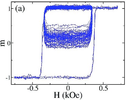
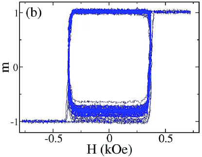
Figure 1: Experimental data of the normalized magnetization, $m$, vs field $H$ for multilayer sample A. Data were taken for two initial saturated loops, 49 loops at amplitude $H_{0}=0.366\pm 0.003$ kOe, and one final saturated loop. (a) Period $P=16.2$ s. (b) $P=38.1$ s. In both cases, the bias field, which is defined and discussed in Section III, was $H_{b}=+1.1\pm 0.5$ Oe.

The hysteresis loops and magnetization time series in samples A and B had very similar characteristics, so we show only those of sample A (the NEPDs for both samples A and B will be presented, however). Figure 1 shows the normalized magnetization, $m$, vs $H$ for periods $P=16.2$ s and $P=38.1$ s in sample A. The initial and final complete loops exhibit full remanent magnetization in a single-domain state, and a sharp reversal region. The loops in the measurement sequence, at field magnitude $H_{0}$, are also square with a sharp reversal region. However, a sharp suppression of the magnetization reversal process is visible below a pinning field $H_{p}=288\pm 2$ Oe (sample B: $H_{p}=260\pm 6$ Oe).pinning.method.endnote The pinning phenomenon has been studied quantitatively in multilayer films, and it is understood to result from a distribution of energy barriers to domain wall motion resulting from lattice defects and variations in the film thickness. Ferré et al. (2004); Lemerle et al. (1998); Della Torre et al. (2002); Chen et al. (2002); Della Torre and Bennett (1998)

The Kerr microscope image in Fig. 2 illustrates the domain reversal pattern in a sister sample, at magnetization $m\approx 0.9$ after nucleation from a positive saturated state. It shows clearly that, above the pinning field $H_{p}$, the reversal within our 1.0 mm² MOKE laser spot occurs by a multidroplet (MD) process Rikvold et al. (1994) of nucleation and growth of approximately circular domains. This reversal pattern is similar to that previously observed in ultrathin, single-layer CoPt films,Ferré et al. (1999) and can be contrasted with the reversal pattern in thicker [Co/Pt]₅₀ multilayers,Davies et al. (2004) in which larger magnetostatic interactions lead to the formation of stripe domains. The MD process is quite similar to that occurring near the DPT in the kinetic Ising model, Korniss et al. (2000) indicating that, if the effect of the pinning field is properly accounted for in the analysis, the kinetic Ising model can serve as a reasonable model of the multilayer.

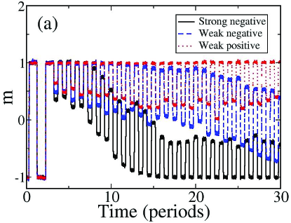
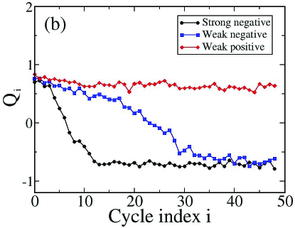
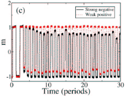
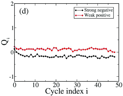
Figure 3: (color online). Time series of the normalized magnetization, $m$, and of the cycle-averaged magnetization, $Q_{i}$, in multilayer sample A, at two different values of the period. (a) Period $P=16.2$ s, magnetization time series. (b) $P=16.2$ s, $Q_{i}$ vs measurement cycle index $i$. (c) $P=38.1$ s, magnetization time series. (d) $P=38.1$ s, $Q_{i}$ vs measurement cycle index $i$. Note that for clarity, only the two initial saturated cycles and the first 26 measurement cycles of the magnetization time series are plotted; however, the full time series of $Q_{i}$ (calculated from the 49 measurement cycles only) are shown. The bias field values corresponding to strong negative, weak negative, and weak positive are $H_{b}=-3.3\pm 0.5,-0.9\pm 0.5,$ and $+1.1\pm 0.5$ Oe, respectively.

As described in Section II, given the important role of the bias field $H_{b}$ as shown in Ref. Robb et al., 2007, we have studied the behavior (the average value and the variance) of $Q$ in the multilayer with respect to both $P$ and $H_{b}$, and compared this to the corresponding behavior of $Q$ in the two-dimensional kinetic Ising model. The two previous experimental reports of the collapse of the hysteresis loop with decreasing field period concentrated principally on the decrease of the hysteresis loop area (cf. Fig. 1 of Ref. Jiang et al., 1995, and Figs. 1 and 2 of Ref. Suen and Erskine, 1997). The cycle-averaged magnetization was also plotted, in Fig. 3 of Ref. Jiang et al., 1995, where its magnitude was shown to become nonzero and then to increase as the applied field amplitude is decreased at a constant value of the field period. However, the bias field, which has a strong effect on the cycle-averaged magnetization near the dynamic phase transition in computational studies Robb et al. (2007) was not carefully controlled, and the variance in the cycle-averaged magnetization was not recorded.

From an initial value of $H_{b}=-3.9$ Oe (sample B: $-7.4$ Oe), the bias field, as generated separately from the time-varying field of the electromagnet, was increased in steps of 0.5 Oe (sample B: steps of $1.1$ Oe). The actual value of the bias field during the 49 measurement cyles was determined, using data from the Hall probe, to fluctuate at the 0.1% level of the applied field amplitude, $H_{0}$. Specifically, the actual bias field could be characterized by a confidence interval $(H_{b}-\Delta H_{b}/2,H_{b}+\Delta H_{b}/2)$, with $\Delta H_{b}=1.0$ Oe.

In Fig. 3(a), magnetization time series for sample A at $P=16.2$ s are shown in a strong negative, weak negative, and weak positive bias field. The corresponding time series, $Q_{i}$, of the cycle-averaged magnetization are plotted in Fig. 3(b). For both negative $H_{b}$ values, the cycle-averaged value of the magnetization (and in fact of any quantity) settles eventually into a non-equilibrium steady state (NESS), so that $Q_{i}$ is observed in Fig. 3(b) to fluctuate around an average value $\langle Q\rangle<0$. (The fluctuations of $Q_{i}$ in the NESS arise from variations in the minor loop amplitude, as seen in Fig.1(a), which are caused principally by thermally-induced fluctuations in the extent and timing of nucleation events.) The transition to the NESS with $\langle Q\rangle<0$ takes longer in the weak negative $H_{b}$ than in the strong negative $H_{b}$, and it does not occur at all in the weak positive $H_{b}$. At the longer period $P=38.1$ s, in contrast, the time series adjust quickly to a NESS with a small $\langle Q\rangle$ value of the same sign as $H_{b}$, as shown in Figs. 3(c) and 3(d). This behavior will be compared to that in the kinetic Ising model in the next section.

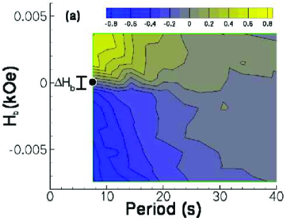
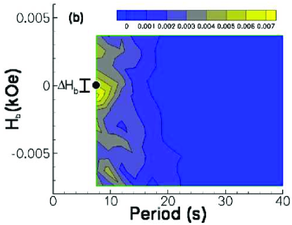
Figure 5: (color online). Same as Fig. 4, but for sample B.

To characterize the behavior of the cycle-averaged magnetization in the multilayer more fully, we measured its average $\langle Q\rangle$ over the field cycles for which the system was in a NESS, for a range of values of $H_{b}$ at each period $P$. We will refer to the resulting contour plot of $\langle Q\rangle$ vs $P$ and $H_{b}$, shown in Fig. 4(a), as a non-equilibrium phase diagram (NEPD), so named in analogy to plots of thermodynamic relationships in equilibrium phase diagrams. As described in Section I, the recent confirmation Robb et al. (2007) of a FDR near the critical point of the DPT in the two-dimensional kinetic Ising model justifies the use of the variance as a proxy for the susceptibility in evaluating evidence for the DPT. The NEPD of the variance $\sigma^{2}(Q)$ within the NESS is shown in Fig. 4(b). The corresponding NEPDs for sample B are presented in Fig. 5. To determine in which field cycle the system should be considered to have entered a NESS, we used the following procedure. The first 10 field cycles were discarded to minimize initial transient effects. We then identified the first subsequent field cycle, $n$, for which the slope of the remaining values $\{Q_{i},i\geq n\}$ could not be statistically distinguished from zero. If more than 15 values of $Q_{i}$ remained, the mean $\langle Q\rangle$ and variance $\sigma^{2}(Q)$ of these values were calculated; otherwise, no data were recorded on the NEPDs for that pair of values $(P,H_{b})$. This procedure ensured that, for example for the measurement sequences in strong negative and weak negative bias fields in Fig. 3(a), the field cycles making up a transition to the NESS with $\langle Q\rangle>0$ were not included as part of the respective NESS’s.

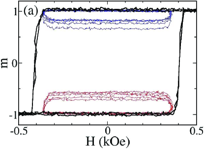
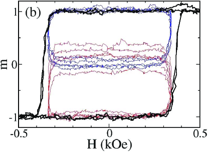
Figure 6: (color online). Normalized magnetization, $m$, vs field, $H$, in (a) sample A at ($P=8.7$ s, $H_{b}=-1.9\pm 0.5$ Oe), and (b) sample B at ($P=7.6$ s, $H_{b}=-0.8\pm 0.5$ Oe). The upper thin lines (blue) show the first 5 measurement cycles, which reach (nominal) positive saturation, while the lower thin lines (red) show the final 5 measurement cycles, which reach (nominal) negative saturation. The thick black lines show two complete cycles at the saturation field, $H_{s}=0.740$ kOe. The nucleation fields in the measurement and saturated cycles correspond closely, except for the increasing branch (from negative saturation) in (a), due to the presence of positively magnetized residual bubble domains in sample A (see text). As the $x$ axis range was reduced to more clearly show the nucleation fields, the saturation loops continue outside the field range shown.

In Fig. 4(a), the boundary between regions with negative $\langle Q\rangle$ and those with positive $\langle Q\rangle$ occurs, for the lower periods, at a slightly negative bias field, $H_{b}\approx-1$ Oe. Similarly, the maximum of $\sigma^{2}(Q)$ occurs, for the lower periods, at a slightly negative bias field, $H_{b}\approx-1.5$ Oe. This appears to contradict the expected $M-H$ inversion symmetry of a ferromagnetic system, which predicts that the NEPDs should be symmetric with respect to the bias field $H_{b}$. However, it can be explained by the presence of residual, hard-to-reverse bubble domains, with coercivities $H_{c}$ in the range $H_{0}<|H_{c}|<H_{s}$, as observed recently in thicker [Co/Pt]₅₀ multilayers.Davies et al. (2004) Since the final saturating field before our measurement sequence begins is positive, such residual domains (if present) would remain positively magnetized during the measurement sequence, in which the field magnitudes $|H(t)|<H_{0}$ would be too weak to reverse them. The bubble domains would then serve as nucleation centers for reversal on the increasing branch of the hysteresis loops during the measurement sequence, lowering the nucleation field on this branch. This effect can indeed be observed in Fig. 6(a), in which the nucleation field $H_{n,+}$ on the increasing branch (from the negatively magnetized state) in the final five measurement cycles is seen to be smaller than the nucleation field in the increasing branch of the cycles at saturation field $H_{s}$. In contrast, the nucleation field $H_{n,-}$ on the decreasing branch (from the positive magnetized state) in the first five measurement cycles is approximately equal to the nucleation field in the decreasing branch of the cycles at saturated field $H_{s}$.

This asymmtery in the nucleation fields has an effect on the value of $Q$ in equal and opposite bias fields, $H_{b}$ and $-H_{b}$, at a given field period in sample A. In the positive bias field $H_{b}$, the reversal window beginning from positive saturation consists of the field intervals $(H_{n,-},-H_{0}+H_{b})$ and $(-H_{0}+H_{b},-H_{p})$, whereas in the negative bias field $-H_{b}$, the reversal window beginning from negative saturation consists of the field intervals $(H_{n,+},H_{0}-H_{b})$ and $(H_{0}-H_{b},H_{p})$. Since $H_{n,+}<-H_{n,-}$, the magnetization reversal proceeds farther in the bias field $-H_{b}$ than in the bias field $+H_{b}$, leading to an asymmetry in the values of the cycle-average magnetization $Q$, with $Q|_{H_{b}}>-Q|_{-H_{b}}$. Thus, the boundary between the regions with negative $\langle Q\rangle$ and positive $\langle Q\rangle$ is shifted from $H_{b}=0$ Oe to the slightly negative bias field $H_{b}\approx-1.0$ Oe.

IV Comparison to kinetic Ising model simulations

We now compare the experimental results to the behavior of the two-dimensional kinetic Ising model with nearest-neighbor ferromagnetic interactions, for which the DPT has been conclusively established, Korniss et al. (2000); Sides et al. (1999) under conditions similar to those of the experiments. The energy of the Ising system is given by

$$E=-J\sum_{\langle i,j\rangle}S_{i}S_{j}-H(t)\sum_{i}S_{i},$$ (3)

with $J>0$ the exchange constant, $H(t)$ the time-dependent magnetic field, and $S_{i}=\pm 1$ the spin magnetic moment at site $i$. We use the Glauber transition rule, $P(S_{i}\rightarrow-S_{i})=1/(1+e^{\beta\Delta E})$, with the next spin to be updated chosen at random. Having verified that larger lattice sizes do not change the results appreciably, we use a $180\times 180$ square lattice with periodic boundary conditions. The Curie temperature of the multilayer was estimated from Ref. Zeper et al., 1991 as $T_{c}\approx 600$ K. We therefore choose the simulation temperature $T=0.5~{}T_{c}$, to correspond to the temperature $T\approx 300~{}K$ of the experiments. As in Ref. Sides et al., 1999, the reversal dynamics are found to be MD for $H_{0}=0.8J$ at this temperature, with mean reversal time $\langle\tau\rangle=59.23\pm 0.06$ Monte Carlo steps per spin (MCSS). For a sawtooth waveform with amplitude $H_{0}=0.8J$, we determine the DPT by finite-size scaling analysis Korniss et al. (2000); Sides et al. (1999) to occur at $P_{c}=493\pm 2$ MCSS.

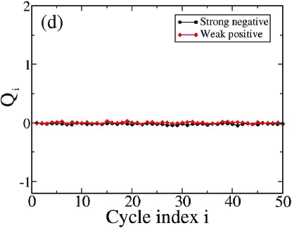
Figure 7: (color online). Time series of normalized magnetization, $m$, and of cycle-averaged magnetization, $Q_{i}$, from simulations of the $L=180$ kinetic Ising model, at two different values of the period and in various bias fields. (a) Period $P=473$ MCSS, magnetization time series. (b) $P=473$ MCSS, $Q_{i}$ vs measurement cycle $i$. (c) $P=1500$ MCSS, magnetization time series. (d) $P=1500$ MCSS, $Q_{i}$ vs measurement cycle $i$. As in Fig. 3, for clarity, only the two initial saturated cycles and the first 26 measurement cycles of the magnetization time series are plotted. However, the full time series of $Q_{i}$, calculated from the 50 measurement cycles, are shown. The bias fields values corresponding to strong negative, weak negative, and weak positive are $-0.013J$, $-0.0035J$, and $+0.0044J$.

To recreate the experimental conditions as closely as possible, we simulated magnetization time series consisting of two saturated loops at $H_{s}=1.6J$, followed by 50 field cycles at $H_{0}=0.8J$. The period values were selected from both below and above $P_{c}$, from $P=368$ to $1575$ MCSS. At each value of $P$, we collected magnetization time series for a range of bias fields from $H_{b}=-0.02H_{0}$ to $0.01H_{0}$. Figures 7(a) and 7(b) show simulated magnetization time series, and the corresponding time series of the cycle-averaged magnetization, $Q_{i}$, for a strong negative, weak negative, and strong positive bias field at period $P=473$ MCSS, just below $P_{c}=493$ MCSS. As in the experimental time series in Figs. 3(a) and 3(b), the transition to the NESS with $\langle Q\rangle<0$ in the simulated time series takes longer in the weak negative $H_{b}$ than in the strong negative $H_{b}$ , and it does not occur at all in the weak positive $H_{b}$. In addition, the behavior of the simulation in strong negative and weak positive $H_{b}$ at the higher period $P=1500$ MCSS, shown in Figs. 7(c) and 7(d), resembles the behavior of the experimental system at higher period shown in Figs. 3(c) and 3(d). The larger splitting between the average values of $\langle Q\rangle$ in Fig. 3(d), relative to Fig. 7(d), is due mainly to the effect of the pinning field in the experimental system, which results in an increased sensitivity to the bias field, as discussed later in this section.

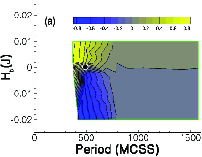
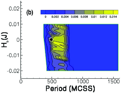
Figure 8: (color online). Non-equilibrium phase diagrams (NEPDs) for the $L=180$ kinetic Ising model, with parameters given in Section IV, of (a) $\langle Q\rangle$ and (b) $\sigma^{2}(Q)$ in a non-equilibrium steady state (NESS), as functions of the period $P$ and bias field $H_{b}$. The data for the NESS were drawn from a single run of 50 field cycles, using the same analysis which was employed for the (experimental) Figs. 4 and 5 and described in Section III. The black dot shows the location of the critical point, $(P=493\pm 2$ MCSS $,H_{b}=0)$, as determined by finite-size scaling analysis.

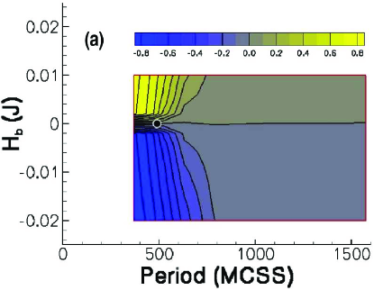
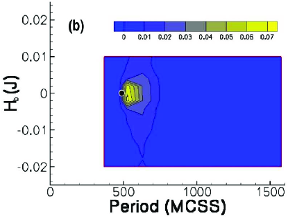
Figure 9: (color online). Same as Fig. 8, but using a different procedure to generate the data in the non-equilibrium steady state (NESS). Here, the data for the NESS were drawn from the final 40 cycles and averaged over 32 independent MC simulations, each of which was initialized in a saturation field of the same sign as its associated $H_{b}$.

The similarity of the simulation data in Fig. 7 to the experimental data in Fig. 3 suggests that the experimental system may be near criticality just above $P=16.2$ s, but this similarity does not by itself provide conclusive evidence of a DPT. To evaluate the question more thoroughly, we constructed NEPDs of $\langle Q\rangle$ and $\sigma^{2}(Q)$, measured in the NESS in simulation, with respect to $P$ and $H_{b}$. Two procedures were used to generate simulation data in a NESS. In the first procedure, we mimicked the experimental data analysis precisely, by identifying the part of the simulated time series which consituted the NESS using the same criterion described in Section III. In the second procedure, the simulation was initialized, for a run at particular values $(P,H_{b})$, such that the final saturation field before the measurement sequence was of the same sign as $H_{b}$. This field-symmetric initial condition begins each simulation near the NESS, for both positive and negative $H_{b}$, thus eliminating the transitions seen in Fig. 3(a). We then ran 32 independent MC realizations of 50 field cycles each, including the final 40 cycles of each realization in the NESS data. The simulated NEPDs of $\langle Q\rangle$ and $\sigma^{2}(Q)$ using the first procedure are shown in Figs. 8(a) and 8(b), respectively, while those produced using the second procedure are shown in Figs. 9(a) and 9(b).

We concentrate first on the comparison of simulation data to the data from experimental sample A, for reasons discussed below. The simulated NEPDs of Fig. 8 are clearly similar in form to the experimental NEPDs in Fig. 4. However, there are two significant differences, which can be accounted for by the presence in sample A of hard-to-reverse, residual bubble domains, and of a pinning field for domain-wall motion, respectively. The first difference is in the position of the peak of the variance $\sigma^{2}(Q)$. In the experimental NEPD, the peak of $\sigma^{2}(Q)$ is situated at ($P\approx 20$ s$,H_{b}\approx-1.5$ Oe), whereas in the simulated NEPD, the (somewhat diffuse) peak occurs at periods just above $P_{c}=493$ MCSS. While one might argue from Fig. 8 that the peak is centered around a slightly negative $H_{b}$, a collection of NEPDs (produced by different MC realizations) showed no net tendency toward either positive or negative $H_{b}$. As described at the end of Section III, the shift in the boundary between the regions of positive and negative $\langle Q\rangle$ values, as well as the shift of the experimental peak of $\sigma^{2}(Q)$, toward negative $H_{b}$, can be explained by the asymmetry in nucleation fields during the measurement sequence. This asymmetry is in turn due to the presence of the residual bubble domains, which were magnetized positively by the final (positive) saturating field before the beginning of the measurement sequence.

The second principal difference between the simulated and experimental NEPDs is the gradual slope of the contour lines extending from the left side of the experimental NEPD in Fig. 4(a), as compared to the steep drop of the corresponding contours in the simulated NEPD in Fig. 8(a). If one normalizes the $H_{b}$ values (i.e., the $y$ axis) by the field magnitude $H_{0}$ in both Figs. 4(a) and 8(a), this difference in slopes becomes even more pronounced. Physically, the difference in slopes corresponds to a susceptibility $\partial\langle Q\rangle/\partial H_{b}$ which falls off more slowly with increasing period in the experiment than in the simulation. This increased sensitivity to the bias field results from the pinning field in the multilayer. In the experiment, the entire magnetization reversal takes place within the restricted field intervals $(-H_{0}+H_{b},-H_{p})$ and $(H_{p},H_{0}+H_{b})$, whereas in the simulated reversal it occurs, albeit with a domain wall velocity decreasing linearly with the applied field, Rikvold and Kolesik (2000) within the entire field intervals $(-H_{0}+H_{b},0)$ and $(0,H_{0}+H_{b})$. A given bias field, expressed as a percentage of $H_{0}$, thus constitutes a larger percentage of the field interval during which magnetization reversal occurs in experiment than in the simulation, and so has a larger effect on $\langle Q\rangle$.

When the second data analysis procedure was used, including averaging over 32 independent simulation runs, the NEPD of $\langle Q\rangle$, shown in Fig.  9(a), became symmetric with respect to $H_{b}$, both above and below $P_{c}$. In addition, the NEPD of $\sigma^{2}(Q)$ in Fig. 9(b) became more sharply focused near $H_{b}=0$ at periods just above $P_{c}$. This strongly suggests that the asymmetry with respect to $H_{b}$ in Fig. 4(a), and size of the peak region in Fig. 4(b), would decrease if the second procedure described above were followed in gathering and analyzing experimental data.

In comparing the simulation data to the results for experimental sample B, we note that in the NEPD of $\langle Q\rangle$ for sample B in Fig. 5(a), there is much less (if any) shift of the boundary between the region of positive $\langle Q\rangle$ and the region of negative $\langle Q\rangle$ toward negative bias field. Similarly, the peak of $\sigma^{2}(Q)$ in Fig.5(b) is just slightly further from $H_{b}=0$ Oe than the uncertainty $\Delta H_{b}/2=0.5$ Oe. The very minimal difference between the nucleation field in the increasing saturating fields and that in the increasing measurement loops in Fig. 6(b), as compared to the sizable difference noted above for sample A in Fig. 6(a), suggests strongly that there were significantly fewer impurities and/or variations in film thickness giving rise to residual bubble domains in sample B. The NEPDs of $\langle Q\rangle$ and $\sigma^{2}(Q)$ for sample B closely resemble the part of the simulated NEPDs (Fig. 8) above $P=500$ MCSS ($\approx P_{c}=493$ MCSS). Thus, we tentatively place the location of the critical period at ($P=7.6$ s, $H_{b}=0.0$ Oe), i.e., at the left edge of the NEPDs, as indicated in Fig. 5. This is also consistent with the fact that the magnetization reversal reaches $m\approx 0$ for sample B at $P=7.6$ s in Fig. 6(b), whereas it reaches only $|m|=0.7$ for sample A at $P=8.7$ s in Fig. 6(a). In simulations, it has been observed Sides et al. (1999) that the DPT occurs at a period where the magnetization reversal (from saturation) proceeds at least as far as $m=0$.

Since the data from sample A includes periods from both below and above our critical period, $P_{c}\approx 20$ s, with the variance $\sigma^{2}(Q)$ visibly decreasing in Fig. 4(b) both below and above this period, we have focused on sample A as our primary evidence for the observation of the DPT. The similarity of the experimental results from sample A to the simulated results, with respect to (i) the behavior of the time series $Q_{i}$ in various $H_{b}$, in Figs. 3 and 7, (ii) the form of the NEPDs of $\langle Q\rangle$, in Figs. 4(a) and 8(a), and (iii) most importantly, the existence of a well-defined peak in the NEPD of $\sigma^{2}(Q)$ in Fig. 4(b); constitute strong evidence for this DPT in an experimental magnetic system. The differences between the experimental and simulated NEPDs of $\langle Q\rangle$ and $\sigma^{2}(Q)$ can be consistently explained, for both samples A and B, in terms of the effect of hard-to-reverse bubble domains in sample A, as described in Section III, and the presence of a pinning field for domain-wall motion, as described earlier in this section.

As mentioned in Section I, the kinetic Ising model we have used does not give rise to a pinning field, and thus presents a simplified model of the motion of domain walls in the [Co/Pt]₃-multilayer. Significant progress has been made in using a Preisach-Arrhenius (PA) model of magnetic viscosity to describe the thermally activated motion of domain walls over a distribution of free-energy barriers associated with variations in film thickness, grain boundaries, and impurities.Della Torre et al. (2002); Chen et al. (2002); Della Torre and Bennett (1998) The PA model, while quite useful to describe phenomenologically the decay of magnetization on long time scales, does not directly incorporate the spatial dependence and cooperative nature of magnetization processes. In addition, recent work Ferré et al. (2004); Lemerle et al. (1998) has shown that the dependence of the energy barriers (to wall motion) on the applied field deviates from the linear dependence Della Torre et al. (2002); Chen et al. (2002); Della Torre and Bennett (1998) usually assumed in PA models. It appears likely that incorporating both spatially varying magnetization, such as that occurring in the MD reversal process (cf. Fig 2), and a realistic description of a wide distribution of energy barriers will require a computationally intensive, multi-scale micromagnetic model, for which the DPT would first have to be established computationally. We have therefore chosen to model the spatially varying MD reversal process faithfully with a two-dimensional kinetic Ising model, and to account for magnetic viscosity effects (i.e., the pinning field) in our analysis and comparison to experiment. The differences between the results of the experiments and the kinetic Ising simulations are consistent with what one would expect from the added effects of magnetic viscosity in an experimental multilayer system exhibiting the DPT.

V Conclusion

We have compared the behavior of the cycle-averaged magnetization, $Q$, in experiments on a [Co/Pt]₃ multilayer, to its behavior in MC simulations of the two-dimensional kinetic Ising model, in which a DPT with respect to the period $P$ of an applied alternating field has been well established. Korniss et al. (2000); Sides et al. (1999) Plots of time series of the magnetization (and of $Q$) in the presence of various bias fields $H_{b}$, as well as non-equilibrium phase diagrams of the average, $\langle Q\rangle$, and the variance, $\sigma^{2}(Q)$, as functions of $P$ and $H_{b}$, were used to characterize and compare the behavior of $Q$ in experiment and simulation. The behavior was seen to be similar, with differences that could be clearly accounted for in terms of the known phenomena of a pinning field and residual bubble domains. The results, in particular the presence of a clear peak in the variance $\sigma^{2}(Q)$ in experimental sample A, provide the strongest experimental evidence to date for the presence of this DPT in a magnetic system. Furthermore, the results strongly suggest that the cycle-averaged magnetization $Q$ serves as a dynamic order parameter in the [Co/Pt]₃-multilayer system.

It would be most desirable to perform further and more precise experiments on the DPT in perpendicular magnetic ultrathin films. Specifically, it would be useful to collect data using the second procedure described in Section IV, i.e., to ensure that the final saturated state before the measurement cycle has the same sign as the applied bias field. Also, one could attempt to apply a field magnitude $H_{0}$ that is significantly larger than the pinning field $H_{p}$, thereby forcing the critical period to lower values. One would expect the effect of the pinning field, for example in creating more gradual contours in the non-equilibrium phase diagram of Figs. 4(a) and 8(a), to be reduced in this case. However, this will be experimentally very challenging given the hysteretic nature and response time of the electromagnet one would need in this case to generate the time-varying applied field sequences.

In addition, a lower value of the critical period would enable the collection of data for more field cycles in each NESS. As noted above, some level of experimental fluctuations in the bias field is probably unavoidable. However, with a sufficiently large number of cycles recorded in a NESS, one could attempt to calculate values of $\langle Q\rangle$ and $\sigma^{2}(Q)$ using data from a subset of the recorded cycles with a more restricted range of $H_{b}$ values. This could potentially supply the precision required to investigate power-law scaling near the critical period. The added statistics provided by forcing the DPT to occur at a shorter period, as well as more precise control over the temporal stability of the bias field, could enable extraction of the critical exponents from the power-law behavior of $\sigma^{2}(Q)$ vs $P-P_{c}$ and $H_{b}$.

Finally, in an ultrathin Au/Co/Au film it was observed Kirilyuk et al. (1997) that a mixture of nucleation at fixed (‘soft’, extrinsic) sites and at random (intrinsic) sites occurred. If this also occurs in [Co/Pt] multilayers, it could affect both the size of the fluctuations of the dynamic order parameter and its spatial correlations, relative to those in the kinetic Ising system, in which nucleation occurs only at random sites. One could examine a series of real-time images of the sample, such as the one shown in Fig. 2, in order to calculate spatial and time-displaced correlation functions to address this question.

The results from such additional experiments could serve to further reinforce the evidence for the DPT presented here. To achieve an even higher degree of confidence, one would need to formulate an accurate, multiscale micromagnetic model of the multilayer, and to demonstrate the existence of the DPT in this computational model. Given the large system sizes needed for computational finite-size scaling analysis, such an effort will likely require innovations in simulation methods, as well as further increases in available computing power.

VI Acknowledgements

The computational work was supported by NSF Grant Nos. DMR-0120310 and DMR-0444051, by the Center for Computational Sciences at Mississippi State University, and by the School of Computational Science at Florida State University. In addition, one of us (D.R.) acknowledges support from Clarkson University and the use of resources under NSF Grant No. DMR-0509104. Another author (A. B.) would like to acknowledge funding from the Department of Industry, Trade and Tourism of the Basque Government and the Provincial Council of Gipuzkoa under the ETORTEK Program, Project IE06-172, as well as from the Spanish Ministry of Science and Education under the Consolider-Ingenio 2010 Program, Project CSD2006-53.

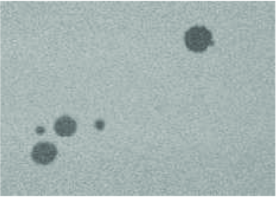
Figure 2: Kerr microscope image of magnetization in a sister [Co/Pt]₃ multilayer sample, taken shortly after the start of magnetization reversal (at $m\approx 0.93$). The area represented in the image had physical dimensions 0.88 $\times$  0.62 mm².

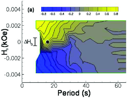
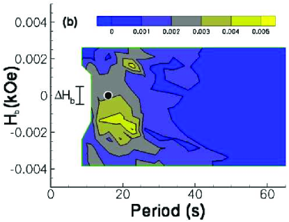
Figure 4: (color online). Non-equilibrium phase diagrams (NEPDs) for sample A, showing (a) the average $\langle Q\rangle$ and (b) the variance $\sigma^{2}(Q)$ in the non-equilibrium steady state (NESS), as functions of the period $P$ and bias field $H_{b}$. The portion of the magnetization time series which consituted the NESS was determined for each ($P,H_{b}$) according to the procedure described in Section III. Within each time series, the bias field fluctuated within a range $(H_{b}-\Delta H_{b}/2,H_{b}+\Delta H_{b}/2)$, with $\Delta H_{b}=1.0$ Oe as shown. The black dot shows the estimated location of the critical point of the DPT.

References

- Woodward et al. (2002) C. E. Woodward, M. Campion, and D. J. Isbister, J. Chem. Phys. 116, 2983 (2002).
- Ogawa et al. (2002) N. Ogawa, Y. Murakami, and K. Miyano, Phys. Rev. B 65, 155107 (2002).
- Kes et al. (2004) P. H. Kes, N. Kokubo, and R. Besseling, Physica C 408-10, 478 (2004).
- Tomé and de Oliveira (1990) T. Tomé and M. J. de Oliveira, Phys. Rev. A 41, 4251 (1990).
- Sides et al. (1999) S. W. Sides, P. A. Rikvold, and M. A. Novotny, Phys. Rev. E 59, 2710 (1999); Phys. Rev. Lett. 81, 834 (1998).
- Korniss et al. (2000) G. Korniss, C. J. White, P. A. Rikvold, and M. A. Novotny, Phys. Rev. E 63, 016120 (2000).
- Chakrabarti et al. (1999) B. K. Chakrabarti and M. Acharyya, Rev. Mod. Phys. 71, 847 (1999).
- Fujiwara et al. (2004) N. Fujiwara, H. Tutu, and H. Fujisaka, Phys Rev. E 70, 066132 (2004).
- Acharyya (2004) M. Acharyya, Phys. Rev. E 69, 027105 (2004).
- Jang et al. (2003) H. Jang, M. J. Grimson, and C. K. Hall, Phys. Rev. B 67, 094411 (2003).
- Meilikhov (2004) E. Z. Meilikhov, JETP Letters 79, 620 (2004).
- Dutta (2004) S. B. Dutta, Phys. Rev. E 69, 066115 (2004).
- Fujisaka et al. (2001) H. Fujisaka, H. Tutu, and P. A. Rikvold, Phys. Rev. E 63, 036109 (2001).
- Jiang et al. (1995) Q. Jiang, H. N. Yang, and G.-C. Wang, Phys. Rev. B 52, 14911 (1995).
- Suen and Erskine (1997) J. S. Suen and J. L. Erskine, Phys. Rev. Lett. 78, 3567 (1997).
- (16) The kinetic Ising model does simplify certain aspects of the magnetization dynamics in the multilayer, mainly the dependence of the domain-wall velocity on the applied field. This issue is discussed in detail in Section IV.
- Hellwig et al. (2003) O. Hellwig, T. L. Kirk, J. B. Kortright, A. Berger, and E. E. Fullerton, Nature Materials 2, 112 (2003).
- Carcia et al. (1985) P. F. Carcia, A. D. Meinhaldt, and A. Suna, Appl. Phys. Lett. 47, 178 (1985).
- Allenspach (1994) R. Allenspach, J. Magn. Magn. Mater. 129, 160 (1994).
- Berger et al. (1995) A. Berger, A. W. Pang, and H. Hopster, Phys. Rev. B 52, 1078 (1995).
- Berger and Erickson (1997) A. Berger and R. P. Erickson, J. Magn. Magn. Mater. 165, 70 (1997).
- Yafet and Gyorgy (1988) Y. Yafet and E. M. Gyorgy, Phys. Rev. B 38, 9145 (1988).
- Bander and Mills (1988) M. Bander and D. L. Mills, Phys. Rev. B 38, R12015 (1988).
- Back et al. (1995) C. Back, C. Würsch, A. Vaterlaus, U. Ramsperger, U. Maier, and D. Pescia, Nature 378, 597 (1995).
- Robb et al. (2007) D. T. Robb, P. A. Rikvold, A. Berger, and M. A. Novotny, Phys. Rev. E 76, 021124 (2007).
- (26) The Hall probe was calibrated accurately by determining the reading of the Hall probe corresponding to true zero field at the sample as the point at which the cycle-averaged magnetization changed from negative to positive value at high field period.
- Davies et al. (2004) J. E. Davies, O. Hellwig, E. E. Fullerton, G. Denbeaux, J. B. Kortright, and K. Liu, Phys. Rev. B 70, 224434 (2004).
- (28) The pinning field was determined by first averaging over a collection of increasing (decreasing) curves, such as the increasing curves near in Fig. 1(a). The widest field range for which all values outside the field range were greater (smaller) than the average value, , within the field range was then found. Finally, the endpoints and from eight such procedures were used to calculate the mean value and uncertainty of given in the text.
- Ferré et al. (2004) J. Ferré, V. Repain, J.-P. Jamet, A. Mougin, V. Mathet, C. Chappert, and H. Bernas, Phys. Stat. Sol. (a) 201, 1386 (2004).
- Lemerle et al. (1998) S. Lemerle, J. Ferré, C. Chappert, V. Mathet, T. Giamarchi, and P. Le Doussal, Phys. Rev. Lett. 80, 849 (1998).
- Della Torre et al. (2002) E. Della Torre, L. H. Bennett, R. A. Fry, and O. A. Ducal, IEEE Trans. Magn. 38, 3409 (2002).
- Chen et al. (2002) A. Chen, R. A. Fry, and E. Della Torre, J. Appl. Phys. 91, 7631 (2002).
- Della Torre and Bennett (1998) E. Della Torre and L. H. Bennett, IEEE Trans. Magn. 34, 1276 (1998).
- Rikvold et al. (1994) P. A. Rikvold, H. Tomita, S. Miyashita, and S. W. Sides, Phys. Rev. E 49, 5080 (1994).
- Ferré et al. (1999) J. Ferré, J. P. Jamet, and P. Meyer, Phys. Stat. Sol. (a) 175, 213 (1999).
- Zeper et al. (1991) W. B. Zeper, H. W. Vankesteren, B. A. J. Jacobs, J. H. M. Spruit, and P. F. Carcia, J. Appl. Phys. 70, 2264 (1991).
- Rikvold and Kolesik (2000) P. A. Rikvold and M. Kolesik, J. Stat. Phys 100, 377 (2000).
- Kirilyuk et al. (1997) A. Kirilyuk, J. Ferré, V. Grolier, J. P. Jamet, and D. Renard, J. Magn. Magn. Mater. 171, 45 (1997).
- (39) Despite applied field magnitudes and bias field magnitudes precise to the 0.5% and 0.1% level, respectively, of the applied field magnitude, it was not possible to establish scaling relations with statistical significance from our data.